2D and 3D Far-Field Radiation Patterns Reconstruction
Based on Compressive Sensing
Berenice Verdin* and Patrick Debroux
Abstract—The measurement of far-field radiation patterns is time consuming and expensive. Therefore, a novel technique that reduces the samples required to measure radiation patterns is proposed where random far-field samples are measured to reconstruct two-dimensional (2D) or three-dimensional (3D) far-field radiation patterns. The proposed technique uses a compressive sensing algorithm to reconstruct radiation patterns. The discrete Fourier transform (DFT) or the discrete cosine transform (DCT) are used as the sparsity transforms. The algorithm was evaluated by using 3 antennas modeled with the High-Frequency Structural Simulator (HFSS) — a half-wave dipole, a Vivaldi, and a pyramidal horn. The root mean square error (RMSE) and the number of measurements required to reconstruct the antenna pattern were used to evaluate the performance of the algorithm. An empirical test case was performed that validates the use of compressive sensing in 2D and 3D radiation pattern reconstruction. Numerical simulations and empirical tests verify that the compressive sensing algorithm can be used to reconstruct radiation patterns, reducing the time and number of measurements required for good antenna pattern measurements.
1. INTRODUCTION
Far-field radiation patterns are an essential part of antenna characterization. Usually, the process of measuring two-dimensional (2D) or three-dimensional (3D) radiation patterns is time consuming and
expensive. For instance, a complete 3D radiation pattern with a spatial resolution in θ and φ of 2◦
requires 16200 measurements. The need for a new technique that will reduce the time required to measure a far-field radiation pattern is thus identified.
Several techniques have been proposed in literature where a small number of near-field samples are taken to reconstruct far-field radiation patterns [1–3]. For these kinds of measurement techniques, the software and hardware to perform near-field measurements are required. In case that only far-field measurements capabilities (software and hardware) are available, then the number of measurements depends on the resolution and accuracy desired.
Compressive sensing has been widely used to overcome sampling restrictions for a wide variety of applications [4–6]. The use of compressive sensing applied to radiation patterns measurements is limited. In [7], a method that uses compressive sensing to reconstruct the antenna radiation pattern is proposed. However, the measurements were performed by using randomly placed sensors which makes the method difficult for practical data measurements. A methodology that reduces the number of samples required in near-field to reconstruct far-field radiation pattern is proposed in [8]. An iterative algorithm is used to find the optimized samples required in near-field. None of these approaches have been applied
to far-field measurements. In our previous work, compressive sensing was used to recover missing
sections of far-field radiation patterns by sampling the available section of the radiation pattern and by using compressive sensing reconstructing the complete radiation pattern [9]. A different application of
Received 3 November 2015, Accepted 6 January 2016, Scheduled 18 January 2016
* Corresponding author: Berenice Verdin ([email protected]).
compressive sensing is presented in this paper, where by using few randomly-distributed samples in the far-field, far-field radiation patterns can be reconstructed.
Specifically, a new measurement technique based on compressive sensing is proposed to perform the measurement and the compression of far-field radiation patterns. The reconstruction algorithm uses the discrete Fourier transform (DFT) or discrete cosine transform (DCT) to recover the patterns. By using the proposed technique a complete reconstruction of either the 2D or 3D radiation pattern is obtained reducing the number of measurements and the time required to characterize an antenna. The number of random measurements required for an optimal reconstruction is calculated by using a priori information obtained from the simulation of the antenna radiation pattern and the compressive sensing algorithm.
2. COMPRESSIVE SENSING THEORY
Consider a signal x of size N ×1 that can be represented in terms of a basis matrixψ of size N ×N.
Then x=ψ−1s, wheres is a vector of size N ×1, andψ−1 is the inverse ofψ. The signal x is said to
be sparse if K (K << N) coefficients of the vector s are non-zero. In such cases, the signal x can be
compressed by using an adequate transform as a basis function [10].
The number of measurements required to reconstruct the signalxcan be reduced by takingy=Ωs
measurements, where y is a vector of size M ×1, M is the number of measurements less than N,
Ω = Aψ, and A is the measurement matrix used to keep the basis functions associated with the
measurements. The approximation of the x signal in the sparse domain, ˆs, is accomplished by solving
the1-minimization problem ˆs= mins1 such thaty=Ωˆs, with the p-norm of a vectorf defined as
fp = (Nj=1|fj|p)1/p, wherep≥1 [10].
2.1. Compressive Sensing Applied to Radiation Patterns
A far-field radiation pattern is a representation of the intensity of the field with respect to θ and φ
given by f(θ, φ). Consider a 2D radiation pattern f(θ) that represents x in the compressive sensing
algorithm. A sparse basis representation s of f(θ) is required to apply the reconstruction compressive
sensing algorithm. Moreover, designing the measurement matrix is a key factor in the radiation pattern recovery using compressive sensing. The measurement matrix used should follow the restricted isometry property (RIP) to ensure recovery [10]. One measurement matrix that has been used in compressive sensing applications that follow the RIP is the random partial Fourier matrix [11–13]. The randomly distributed partial Fourier matrix is derived from the DFT given by
F(k) =
N−1
n=0
f(n)e−j2πkn/N, (1)
where n is the index of the radiation pattern angle, k the index of the transform domain, and N the
total number of samples.
In the case of a measured far-field radiation pattern,f(θ) is a vector of size N ×1; therefore, the
DFT can be represented as an operator in matrix form such that s=ψx, where s is in the transform
domain that containsK < N non zero values, andψ is the matrix representation of the DFT given by
ψDF T = ⎡ ⎢ ⎣
e−j2πn0k0/N . . . e−j2πn0kN−1/N
..
. . .. ...
e−j2πnN−1k0/N . . . e−j2πnN−1kN−1/N
⎤ ⎥
⎦. (2)
Another transform that can be used as a basis function is the discrete cosine transform (DCT). The DCT can be performed by using a matrix defined as
ψDCT =
⎡ ⎢ ⎢ ⎢ ⎢ ⎣
1 . . . 1
cos
α
0n1π
2N
. .. cos
(αN−1n1)π
2N
cos
α
0nN−1π
2N
. . . cos
(αN−1)nN−1π
2N ⎤ ⎥ ⎥ ⎥ ⎥
whereαq= 2kq+ 1.
The DFT or DCT matrix can be converted to a partial random matrix by randomly selecting the rows of the DFT or DCT matrices [13, 14]. The random rows are created by using a uniform
random distribution. The measurement of the radiation pattern is performed by using M number of
measurements where M < N yielding a basis matrix Ω with dimensions M ×N. As can be seen,
sensing of the radiation pattern is already incorporated into the compressive sensing algorithm, where
just M samples are randomly measured. Ultimately, the measured samples are used as the input to
the compressive sensing algorithm to reconstruct the radiation pattern with a minimal reconstruction error.
In the case of 3D radiation patterns,f(θ, φ), the goal is to reduce the number of samples in both the
θ andφdirections. A traditional 2D compressive sensing algorithm converts the matrix into a long 1D
vector to perform the reconstruction. Although this may work for other applications [10], vectorizing the matrix will reduce the number of measurements in only one direction and will add complexity to the reconstruction in the radiation pattern. A method where parallel compressive sensing is used in order to overcome vectorization limitations was proposed in [15], where the reconstruction is performed by using compressive sensing column by column. By using this method, however, the reduction of the number of measurements is performed only in one direction.
Assume that the matrix containing the 3D radiation pattern information is a matrix N ×L. A
two-step process is proposed, where random measurements are taken in both directions resulting in a
matrixM×P, whereM < N andP < L, obtaining a reduction of the measurements needed in bothθ
and φdirections. The 3D radiation pattern reconstruction is performed first in theφdirection for each
measured θ, where each 2D cut is reconstructed using parallel compressive sensing for each row [15].
Then, the 2D cuts are reconstructed by using the columns of the matrix resulting into a 3D radiation
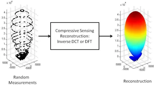
pattern with size N ×L. A representation of the measurement technique is shown in Fig. 1, where
randomly-distributed samples are taken to reconstruct the far-field radiation pattern using compressive sensing.
Figure 1. Compressive sensing algorithm for 3D radiation patterns.
The number of measurements required to successfully reconstruct an antenna radiation pattern is depended on the type of antenna used. Therefore, a priori information is required. This information is obtained by simulating the far-field radiation pattern and the number of samples required to successfully reconstruct the radiation pattern with low error as shown in the following sections. Once the number of measurements needed is identified, the randomly-distributed samples can be sorted to perform the anechoic chamber measurements to reduce the time required to take the measurements.
error (RMSE) is used, defined as
RMSE=
1
N N
n=1
(fn−ˆfn)2, (4)
where fn is the simulated or measured radiation pattern point and ˆfn the compressive sensing
reconstruction of the radiation pattern point.
3. EVALUATION OF THE COMPRESSIVE SENSING RECONSTRUCTION ALGORITHM BY SIMULATION
The compressive sensing algorithm was evaluated by using 3 antennas: the half-wave dipole, the Vivaldi
and the pyramidal horn. The total far-field electric field radiation patterns of the antennas were
simulated in HFSS. Compressive sensing was applied to reconstruct the radiation pattern for each antenna with limited data points. The half-wave dipole and the horn antennas were modeled with a
frequency of 1.35 GHz, and the Vivaldi antenna was modeled at 6 GHz. The electrical size of the
half-wave dipole was 0.5, the horn antenna was 1.566, and the Vivaldi ranged from 0.166 to 1.278. The 2D
radiation pattern for each antenna was simulated at a resolution of 2◦; therefore, the total number of
samples to be reconstructed is thus considered to be 180. Sketches of the HFSS models of the antennas are shown in Fig. 2. A test coaxial cable (CBL Mini-Circuits) was included in the model for each antenna. For a better visualization, the antennas are not scale with respect to each other.
Figure 2. Antennas used to evaluate the compressive sensing algorithm.
0.2 0.4
0.6 0.8
1
30
210
60
240
90
270 120
300 150
330
180 0
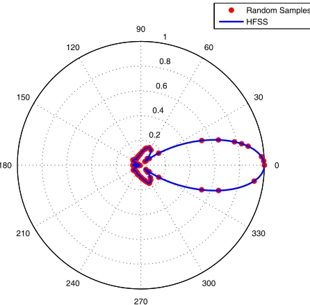
Random Samples HFSS
Figure 3. Randomly distributed measurements taken from the simulated radiation pattern of a
horizonal half-wave dipole at φ= 0.
0.2 0.4
0.6 0.8
1
30
210
60
240
90
270 120
300 150
330
180 0
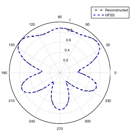
Reconstructed HFSS
Figure 4. Simulated and reconstructed radiation patterns of a horizonal half-wave dipole
3.1. Half-Wave Dipole Antenna
Figure 3 shows the simulated 2D far-field radiation pattern for φ = 0. Superimposed on the pattern
are the samples used for reconstruction. The reconstructed radiation pattern using the DFT matrix for the compressive sensing reconstruction algorithm is shown in Fig. 4. In this case 50 samples where used to reconstruct the radiation pattern, that is 27% of the total number of samples with an RMSE of 2×10⁻³.
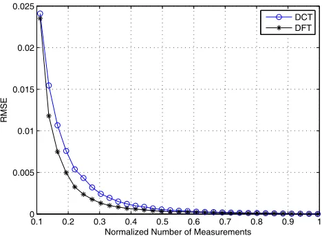
There is a tradeoff between the number of measurements required to obtain a reconstruction of the radiation pattern and the RMSE of that reconstruction. Since a random distribution of measurements is used in the compressive sensing reconstruction, a Montecarlo simulation was performed where the RMSE of reconstruction was calculated as the number of measurements M was increased. The experiment was repeated 1000 times for each number of measurements and the RMSE averaged over the simulations. Fig. 5 shows the RMSE with respect to the normalized number of measurements using the DFT and the DCT. The reconstruction converges to the radiation pattern faster when using the DFT. This plot is used as a priori information to define the number of measurements required for a given RMSE.
0.1 0.2 0.3 0.4 0.5 0.6 0.7 0.8 0.9 1 0
0.005 0.01 0.015 0.02 0.025
Normalized Number of Measurements
RMSE
DCT DFT
Figure 5. A Montecarlo simulation of the RMSE of the reconstructed radiation pattern for the
horizontal half-wave dipole for φ= 0.
3.2. Vivaldi Antenna
The half-wave dipole has a simple radiation pattern that can be very well reconstructed by using the proposed compressive sensing algorithm. A more complicated far-field radiation pattern was obtained
by modeling a Vivaldi antenna. The H-plane principal cut of the 2D radiation pattern of the Vivaldi
antenna was simulated with HFSS. The radiation pattern and the randomly distributed samples used for the compressive sensing reconstruction are shown in Fig. 6.
The reconstructed radiation pattern is shown in Fig. 7. In this case the DFT and 70 samples were used for reconstruction, 38% of the total samples that are required to obtain a reconstruction with a RMSE of 2.5×10⁻³.
The RMSE was calculated by a Montecarlo simulation of 1000 realizations as the normalized number of measurements increased. Fig. 8 shows the RMSE comparison of the DFT and the DCT compressive sensing algorithms. It is seen that the RMSE of the reconstruction obtained when using the DFT converges to zero faster. However, due to the relative complexity of the pattern, more samples are required to obtain a good reconstruction compared to the half-wave dipole antenna pattern.
3.3. Pyramidal Horn Antenna
0.2 0.4
0.6 0.8
1
30
210
60
240
90
270 120
300 150
330
180 0
Random Samples HFSS
Figure 6. Simulated radiation pattern and randomly distributed samples used for the reconstruction of the Vivaldi antenna.
0.2 0.4
0.6 0.8
1
30
210
60
240
90
270 120
300 150
330
180 0
Reconstructed HFSS
Figure 7. Simulated and reconstructed radiation patterns of the Vivaldi antenna.
0.1 0.2 0.3 0.4 0.5 0.6 0.7 0.8 0.9 1
0 0.01 0.02 0.03 0.04 0.05 0.06 0.07 0.08
RMSE
DFT DCT
Figure 8. A Montecarlo simulation of the RMSE of the reconstructed radiation pattern of the Vivaldi antenna.
points. This yielded an RMSE of 1.3×10⁻³.
Figure 10 shows the simulated radiation pattern compared to the reconstructed radiation pattern. A good approximation of the radiation pattern of the horn antenna is obtained.
The RMSE was calculated as the number of measurements was increased. A Montecarlo simulation of 1000 trials was used to obtain the RMSE of the radiation pattern reconstructed with the DFT and
the DCT as a function of measurement points, M, used. The results are shown in Fig. 11. The two
reconstruction basis matrices give similar results as they converge to zero with approximately the same number of measurements.
The 3D radiation pattern reconstruction of the horn antenna was evaluated by using the number of points required for a given acceptable RMSE as found in Fig. 11. A Montecarlo simulation was performed
where the number of measurements along the θ was fixed to 30 as the number of measurements along
φwas increased. The RMSE was calculated for each 2D radiation pattern cut f(φ) of the 3D pattern.
The process was repeated 100 times to obtain the RMSE for eachφas the number of measurements was
0.2 0.4 0.6 0.8 1 30 210 60 240 90 270 120 300 150 330 180 0 Random Samples HFSS
Figure 9. Simulated radiation pattern and randomly distributed measurements used for reconstruction of the horn antenna.
0.2 0.4 0.6 0.8 1 30 210 60 240 90 270 120 300 150 330 180 0 Reconstructed HFSS
Figure 10. Simulated and reconstructed radiation patterns of the horn antenna.
0.1 0.2 0.3 0.4 0.5 0.6 0.7 0.8 0.9 1 0 0.005 0.01 0.015 0.02 0.025 0.03 0.035 0.04 0.045 0.05 RMSE
Normilized Number of Measurements
DFT DCT
Figure 11. A Montecarlo simulation of RMSE of the reconstructed radiation pattern of the horn antenna.
Normalized Number of Measurements 0.2 0.4 0.6 0.8 1 20 40 60 80 100 120 140 160 0.1 0.2 0.3 0.4 0.5 0.6 0.7 0.8 0.9 φ
Figure 12. RMSE of the reconstructed 3D radiation pattern of the measured pyramidal horn antenna using the DFT.
approaches zero after 0.4 normalized or 40% of the number of measurements. The RMSE is higher at
the region where φis close to zero.
4. EMPIRICAL EVALUATION OF THE COMPRESSIVE SENSING RECONSTRUCTION ALGORITHM
A pyramidal horn antenna (having the same dimensions as the horn antenna simulated in HFSS) was measured to test the compressive sensing algorithm empirically. The transmitted frequency used was
1.35 GHz. In order to test the compressive sensing reconstruction algorithm, the radiation pattern was
5 hours in our anechoic chamber. The measured 2D radiation pattern and the randomly distributed samples used for reconstruction are shown in Fig. 13. Note the lack of back lobe measurement due to presence of the supporting tower in the anechoic chamber in addition thermal noise is being added to the experiment because of the hardware used.
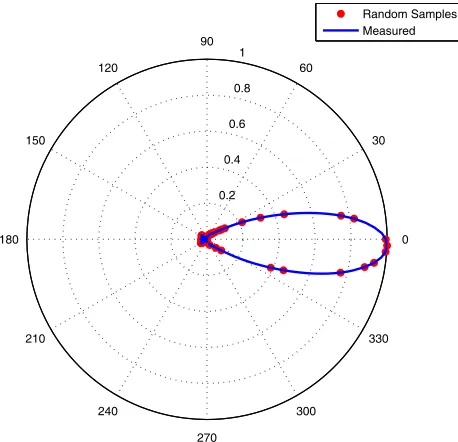
The simulated a priori information was used to identify the number of samples required for a good reconstruction. Based on Fig. 11, 80 samples, that is 46% of the total samples, were used for the reconstruction (the same number of samples used in the simulated radiation pattern of the horn antenna). The 2D radiation pattern reconstruction and the measured radiation pattern are shown in Fig. 14.
Figure 15 shows the empirical radiation pattern and the randomly distributed samples used to
reconstruct the radiation pattern. The compressive sensing algorithm was applied in θ and in φ. A
0.2 0.4
0.6 0.8
1
30
210
60
240
90
270 120
300 150
330
180 0
Random Samples Measured
Figure 13. 2D radiation pattern of the mea-sured pyramidal horn antenna and the random measurement samples used for reconstruction.
0.2 0.4
0.6 0.8
1
30
210
60
240
90
270 120
300 150
330
180 0
Reconstruction Measured
Figure 14. Measured and reconstructed radia-tion patterns of the pyramidal horn antenna.
Figure 15. The empirical 3D radiation pattern and randomly distributed samples used for the reconstruction of the pyramidal horn antenna.
reduced number of measurements was used in both direction: 30 measurements were used alongθ and
70 measurements were used along φ. The number of measurements were chosen a priori. Since the
DFT and the DCT provide similar results when reconstructing radiation pattern of the horn antenna, only the DFT was used for the 3D reconstruction. A total of 2100 samples taken randomly from a total of 16200 samples were used to reconstruct the 3D pattern. The reconstructed 3D radiation pattern is shown in Fig. 16. The compressive sensing reconstruction reproduces the original radiation pattern very well.
5. CONCLUSIONS
A compressive sensing algorithm that performs the reconstruction of 2D or 3D far-field radiation patterns was presented. The compression rate, and thus the number of random measurements required for a good reconstruction, depends on the complexity of the radiation pattern structure. It was observed that as the complexity of the antenna increased, the number of measurements required for a good reconstruction also increased. Two basis matrices, the DFT and the DCT, were evaluated for the reconstruction of radiation patterns. It can be concluded that the DFT matrix performs a better reconstruction of the radiation patterns. Information about the number of samples required to reconstruct the radiation pattern is obtain by simulating the radiation pattern and running the compressive sensing algorithm a priori. Numerical simulations indicates that 2D or 3D radiation patterns can be reconstructed using between 20% and 44% of the total number of measurements.
The algorithm was evaluated empirically on a pyramidal horn antenna, where 2D and 3D radiation
patterns measured in an anechoic chamber were reconstructed well. The proposed reconstruction
algorithm can thus be used to reconstruct 2D or 3D radiation patterns with a reduced number of required far-field measurements. This, in turn, reduces the time required to take the measurements.
The implementation of the algorithm requires the implementation of a new measurement paradigm that will perform random measurements in the anechoic chamber. By using the proposed methodology, the time required to measure radiation patterns can be reduced without significant loss of accuracy. The number of measurements required to obtain a good reconstruction using compressive sensing depends on the complexity of the radiation pattern. That is, it depends on the number of K non-zero coefficients in the sparsity domain representation of the radiation patterns.
ACKNOWLEDGMENT
Research was supported by the Army Research Laboratory and was accomplished under Cooperative Agreement Number W911NF-12-2-0019.
REFERENCES
1. Hansen, J. E., Spherical Near-field Antenna Measurement, The Institution of Engineering and
Technology, United Kingdom, 1988.
2. D’Agostino, F., F. Ferrara, C. Gennarelli, R. Guerriero, and M. Migliozzi, “Far-field reconstruction
from a minimum number of spherical spiral data using effective antenna modelings,” Progress in
Electromagnetics Research B, Vol. 37, 43–58, 2012.
3. Farouq, M., M. Serhir, and D. Picard, “Matrix method for far-field calculation using irregular
near-field samples for cylindrical and spherical scanning surfaces,” Progress In Electromagnetics
Research B, Vol. 63, 35–48, 2015.
4. Romberg, J., “Imaging via compressive sampling,” IEEE Antennas Propag. Mag., Vol. 25, No. 2,
14–20, 2008.
5. Trzasko, J., A. Manduca, and E. Borisch, “Highly under sampled magnetic resonance image
reconstruction via homotopic ell-0-minimization,” IEEE Trans. Med. Imag., Vol. 28, No. 1, 106–
121, 2009.
6. Baraniuk, R. and P. Steeghs, “Compressive radar imaging,” IEEE Radar Conf., Waltham,
7. Carin, L., D. Liu, and B. Gua, “In situ compressive sensing,” IEEE Science Inverse Problems, Vol. 24, 2008.
8. Giordanengo, G., M. Righero, F. Vipiana, G. Vecchi, and M. Sabbadini, “Fast antenna testing with
reduced near field sampling,” IEEE Transactions on Antennas and Propagation, Vol. 62, No. 5,
2501–2513, 2014.
9. Verdin, B. and P. Debroux, “Reconstruction of missing sections of radiation patterns using
compressive sensing.”IEEE International Symposium, 780–781, 2015.
10. Baraniuk, R., “Compressive sensing,”IEEE Signal Process. Mag., Vol. 24, 118–121, 2007.
11. Candes, E. J., T. Tao, and J. Romberg, “Robust uncertainty principles: Exact signal reconstruction
from highly incomplete frequency information,” IEEE Trans. on Inf. Theory, Vol. 52, No. 2, 489–
509, 2006.
12. Candes, E. J. and T. Tao, “Near optimal signal recovery from random projections: Universal
encoding strategies?,” IEEE Trans. on Inf. Theory, Vol. 52, No. 12, 5406–5425, 2006.
13. Fornasier, M. and H. Rauhut, “Compressive sensing,” Handbook of Mathematical Methods in
Imaging, 187–228, 2010.
14. Rauhut, H., “Compressive sensing and structural random matrices,” Theoretical Foundations and
Numerical Methods for Sparse Recovery, 1–91, 2010.
15. Fang, H., S. S. Vorobyov, H. Jiang, and O. Taheri, “Permutation meets parallel compressed sensing:
How to relax restricted isometry property for 2D sparse signals,”Proc. Inst. Elect. Eng. 12th Int.