Accurate and efficient explicit approximations of the
Colebrook flow friction equation based on
Wright-Omega function
Dejan Brkić 1,2,* and Pavel Praks 1,3,*
1 European Commission, Joint Research Centre (JRC), Directorate C: Energy, Transport and Climate, Unit
C3: Energy Security, Distribution and Markets, Via Enrico Fermi 2749, 21027 Ispra (VA), Italy
2 Alfatec, Bulevar Nikole Tesle 63a, 18000 Niš, Serbia
3 IT4Innovations National Supercomputing Center, VŠB—Technical University of Ostrava, 17. listopadu
2172/15, 708 00 Ostrava, Czech Republic
* Correspondence:
[email protected] (D.B.); [email protected] or [email protected] (P.P.)
Abstract: The Colebrook equation is a popular model for estimating friction loss coefficients in
water and gas pipes. The model is implicit in the unknown flow friction factor . To date, the
captured flow friction factor can be extracted from the logarithmic form analytically only in the term of the Lambert -function. The purpose of this study is to find an accurate and computationally efficient solution based on the shifted Lambert -function also known as the
Wright -function. The Wright -function is more suitable because it overcomes the problem with the overflow error by switching the fast growing term = ( ) of the Lambert -function to the series expansions that further can be easily evaluated in computers without causing overflow run-time errors. Although the Colebrook equation transformed through the Lambert -function is
identical to the original expression in term of accuracy, a further evaluation of the Lambert -function can be only approximate. Very accurate explicit approximations of the Colebrook equation that contains only one or two logarithms are shown. The final result is an accurate
explicit approximation of the Colebrook equation with the relative error of no more than 0.0096%. The presented approximations are in the form suitable for everyday engineering use, they are both
accurate and computationally efficient.
Keywords: Colebrook equation; hydraulic resistance; Lambert -function; Wright -function;
explicit approximations; computational burden; turbulent flow; friction factor.
1. Introduction
The Colebrook equation; Eq. (1), is an empirical relation which in its native form relates implicitly the unknown Darcy’s flow friction factor with the known Reynolds number and the known relative roughness of inner pipe surface ∗ [1,2]. Engineers use it at defined domains of the
input parameters: 4000< <108 and for 0< ∗<0.05. The Colebrook equation is transcendental (cannot be expressed in the term of elementary functions), the implicitly given function in respect to the
unknown flow friction factor
= −2 ∙ . ∙ + ∗
. , (1)
The Colebrook equation; Eq. (1) has also an exact explicit analytical form in the term of the Lambert -function; Eq. (2) [3,4] that is also transcendental, but which can be evaluated through
the numerous thoroughly tested procedures of various accuracy and complexity developed for various applications in physics and engineering [5].
= ( )·
. · ( )
+ ( ) − =
. · ( )
+ ·∗
. · . ·
( ) , (2)
The parameter in Eq. (2) depends on the input parameters; the Reynolds number and the
relative roughness of inner pipe surface ∗. Its domain is 7.51< <618187.84. The Lambert -based Colebrook equation; Eq. (2), contains the fast growing term ( ), which cannot be stored in computer registers due to the runtime overflow error for the certain combinations of the Reynolds number and the relative roughness of inner pipe surface ∗ that can easily occur in everyday engineering practice [6,7]. The problem can be solved using the Wright -function, a cognate of the
Lambert -function, which uses a shifted, not fast-growing argument [4,8,9].
This paper presents few approximate solutions of the transformed Lambert -based
Colebrook equation in the form more suitable for computing codes used in various engineering software. The best version of the presented explicit approximation gives the value of flow friction
factor f, for which the Colebrook equation is in balance with the relative error of no more than 0.0096%. Such accuracy achieved without using a large number of computationally expensive
logarithmic functions (or non-integer powers) is highly computationally efficient. As reported by Clamond [10], Winning and Coole [11], Biberg [4], Vatankhah [12], etc., functions such as
logarithms and non-integer powers require special algorithms with execution of many more floating-point operations compared with the basic arithmetic operations (+,-,*,/) that are executed directly in the Central Processor Unit (CPU) of computers. Apparently, this is the first highly
accurate explicit approximation of the Colebrook equation that contains only two computationally expensive functions (two logarithms or as an alternative two functions with non-integer powers) or
even less if a combination of Padé approximations [13,14] and symbolic regression is used for a further reduction of the computational burden (where as a result one of the logarithms is
approximated by simple rational functions with moderate increase of the maximal relative error).
2. Proposed explicit approximations and comparative analysis
The Colebrook equation in the term of the Lambert -function was apparently first proposed in 2018 by Keady [3]. However, as confirmed by Sonnad and Goudar [6] and Brkić [7], the term
( ) grows so fast that cannot be evaluated easily even in registers of modern computer due to the overflow runtime error for a certain number of combinations of the input parameters; the
Reynolds number and the relative roughness of inner pipe surface ∗; where parameter of equation (2) depends directly on them. The here shown procedure replaces this fast growing term by the much more numerically stable Wright -function [15]. As noted by Lawrence et al. [15], the
Further about the Colebrook equation transformed in explicit form in term of the Lambert -function can be found in Keady [3], Goudar and Sonnad [18,19], Brkić [20-23], More [24], Sonnad
and Goudar [25,26], Clamond [10], Rollmann and Spindler [9], Mikata and Walczak [27], Biberg [4], Vatankhah [12], etc.
2.1. Transformation and formulation
The shifted Wright -function transforms the argument to in the series ( ) = ( ) ≈ ( ) − ( ( )) + ((( ))); where = ( ). In that way, the undesirably fast growing term
( ) in Eq. (2) is approximated accurately through ≈ − ( ) + ( ). The transformation is based on unsigned Stirling numbers of the first kind as reported by Rollmann and Spindler [9].
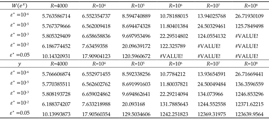
Table 1 shows values of ( ) compared with its approximate replacement in the domain of applicability of the Colebrook equation. Without the proposed transformation and simplification, the runtime overflow error occurs during the evaluation of the friction factor in computers for
certain pairs or the Reynolds number and the relative roughness of inner pipe surface ; where parameter x of Eq. (2) depends directly on them (#VALUE! is overflow error in Table 1). The values
in Table 1 are calculated in MS Excel.
Table 1. Values of ( ) compared with its approximate replacement ≈ − + .
( ) R=4000 R=104 R=105 R=106 R=107 R=108
∗=10-6
5.763586714 6.552354737 8.594740889 10.78188015 13.94025768 26.71930109
∗=10-5
5.767379666 6.562009418 8.694474328 11.80401384 24.50329461 125.7849498
∗=10-3
5.805329409 6.658658836 9.697953496 22.29514802 124.0554132 #VALUE!
∗=10-2
6.186774452 7.63459358 20.09639172 122.325789 #VALUE! #VALUE!
∗=0.05
10.14320931 17.90904123 120.5960672 #VALUE! #VALUE! #VALUE!
R=4000 R=104 R=105 R=106 R=107 R=108
∗=10-6
5.766606874 6.552971455 8.592338256 10.7784212 13.93654591 26.71669441
∗=10-5
5.770385511 6.562602762 8.691991603 11.80037821 24.50049484 136.3596559
∗=10-3
5.808193728 6.659024862 9.694862641 22.29214094 134.073966 1246.853296
∗=10-2
6.188374207 7.633218988 20.093168 131.7885643 1244.552558 12371.62215
∗=0.05
10.13993873 17.90560354 129.5034606 1242.251823 12369.31975 123639.9564 #VALUE! – Overflow error
The simplifications; ( ) − ≈ ( ) · − 1 ; ≈ 0.8686; · . ≈ 2.18; and 2.18 · 3.71 ≈ 8.0878, transform the Lambert -based expression of the Colebrook equation in a very accurate explicit approximate form that can be used efficiently in everyday engineering practice; Eq. (3):
≈ 0.8686 · + ( + ) · − 1 ≈ · ∗
.
≈
. ≈ ( ) − 0.779397488 ⎭
⎪ ⎬ ⎪ ⎫
Instead of logarithmic functions in the proposed explicit approximation; Eq. (3), a new form for and ( + ) can be introduced, where can be any sufficiently large constant, where the larger value of gives the more accurate approximation of logarithmic function, Eq. (4):
≈ ·
. −
ln( + ) ≈ · ( + ) −
, (4)
Very accurate results are obtained for > 10 . Choosing this value, power = is a fraction with integer numerator and denominator, where the appropriate form depends on the programming language and the option with fever floating point operations should be chosen [28].
The forms such as . .
requires evaluation of two transcendental functions because
compilers in most programming languages interpret it through . · . [10].
For more accurate results ( ) − ≈ . · ( ). − ln( ) or ( ) − ≈ . · ( )− ln( ) +
( ) .
can be used. These new approximations were found by symbolic regression software
Eureqa [29-31] and they are 2.5 and 16.7 times respectively more accurate compared with the expression from Table 1. The related approximations are given with Eq. (5) and Eq. (6),
respectively.
≈ 0.8686 · + . · ( )
. − ( + ), (5)
≈ 0.8686 · + . · ( )− ( + ) + ( ( ) ). , (6) In Eq. (5) and Eq. (6), parameters and are the same as in Eq. (3).
2.2. Accuracy
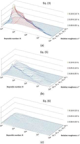
With the friction factor f computed using the approximate equations Eq. (3), the Colebrook equation is in balance with the relative error of no more than 0.13%, while using Eq. (5) of no more than 0.045%, and finally, using Eq. (6) of no more than 0.0096%, respectively. Related distribution of
errors is shown in Figure 1. The presented approximations require evaluation of only two computationally expensive functions (two logarithms; Eq. (3), Eq. (5) and Eq. (6) or alternatively
two non-integer powers; Eq. (4)), and therefore they are not only accurate, but also efficient for calculation.
The here shown approximation; Eq. (3) based on the Wright -function with the relative error up to 0.13% is about ten times more accurate compared with the approximation from Brkić [22],
(a)
(b)
(c)
Figure 1. Distribution of the relative error by the proposed explicit approximation of Colebrook’s
equation; (a): Eq. (3), (b): Eq. (5) and (c): Eq. (6); Comparison
The most accurate approximations available up to date are by Vatankhah [12], Buzzelli [32], Vatankhah and Kouchakzadeh [33], Romeo et al. [34], Zigrang and Sylvester [35] and Serghides
Further about accuracy of explicit approximations to the Colebrook equation can be found in Zigrang and Sylvester [37], Gregory and Fogarasi [38], Brkić [39,40], Winning and Coole [11,41],
Brkić and Ćojbašić [42].
2.3. Complexity and computational burden
In computer environment, a logarithmic function and non-integer powers require more
floating-point operations to be executed in the CPU compared with the simple arithmetic operations such as adding, subtracting, multiplication or division [10-12]. With the relative error of
up to 0.0096%, the here proposed explicit approximation of the Colebrook equation; Eq. (6), that contains only two computationally expensive functions, is not only accurate but also sufficiently
efficient. Winning and Coole [11] reported relative effort for computation as: Addition-1, Subtraction-1.18, Division-1.35, Multiplication-1.55, Squared-2.18, Square root-2.29, Cubed-2.38,
Natural logarithm-2.69, Cubed root-2.71, Fractional exponential-3.32, and Logaritm to base 10-3.37. On the other hand, Biberg [4] adds division in the group of more expensive functions.
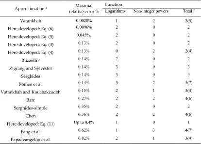
For comparison, Table 2 provides number of logarithmic functions and non-integer terms used
in available approximations. Table 2 shows only highly accurate approximations with the relative error of no more than 1% according to criterions set by Brkić [29]. All approximations from Table 2
are given in Appendix of this article.
Table 2. Number of computationally expensive functions in the available approximations of the
Colebrook equations that introduce relative error of no more than 1%.
Approximation 1 Maximal
relative error %
Function
Logarithms Non-integer powers Total 2
Vatankhah 0.0028% 1 2 3(5)
Here developed; Eq. (6) 0.0096% 2 0 2
Here developed; Eq. (5) 0.045%, 2 0 2
Here developed; Eq. (3) 0.13% 2 0 2
Here developed; Eq. (4) 0.13% 0 2 2(4)
Buzzelli 3 0.14% 2 0 2
Zigrang and Sylvester 0.14% 3 0 3
Serghides 0.14% 3 0 3
Romeo et al. 0.14% 3 2 5(7)
Vatankhah and Kouchakzadeh 0.15% 2 1 3(4)
Barr 0.27% 2 2 4(6)
Serghides-simple 0.35% 2 0 2
Chen 0.36% 2 2 4(6)
Here developed; Eq. (11) Up to 0.4% 1 0 1
Fang et al. 0.62% 1 3 4(7)
Papaevangelou et al. 0.82% 2 1 3(4)
1 All approximations are listed in Appendix of this paper, 2 in brackets: according to Clamond [10]
non-integer powers require evaluation of two computationally expensive functions – logarithm and
In addition to the here presented, the approximation by Brkić [22,23] is also based on the Lambert W-function, but with four logarithmic functions used, it is also much more
computationally expensive (with the relative error of about 2.2% it is also significantly less accurate).
In the next Section, the logarithmic function of ≈
. from Eq. (3) is approximated very
accurately trough rational polynomial expression, so complexity and computational additionally
decrease. Also, subtraction requires less floating-point operations than division, so the computational cheaper form ≈ ( ) − 0.779397488 should be used instead.
2.4. Simplifications
A simple rational approximation of the logarithm term of the novel Colebrook
approximation formulas; Eq. (3), Eq. (5) and Eq. (6), is shown in this Section. The logarithm represents the most computationally expensive operation of the Colebrook formula, while the most its approximations also contain computationally demanded non-integer power terms. In order to
reduce computation costs, the idea is to replace the term that contains the logarithmic function by simple rational functions. A combination of Padé approximation [14,43] and an artificial intelligence
symbolic regression procedure [29-31,] is used for this. Although the logarithm is a transcendental function, the found rational approximation remains simple and accurate with the maximal relative
error limited to 0.2%. Although this rational approximation of the logarithm is not very nice for a human perception, it is very fast at computers, as it requires only a limited number of basic
arithmetic operations to be executed in the CPU.
For the purpose of this simplification, the observed form from Eq. (3) can be transformed as;
Eq. (7):
≈ ln( ) − ln(2.18) = ln(315012.6 · ) − 0.77932 = ln( ) + ln(315012.6) − 0.77932 = ln( ) + 11.881, (7)
In Eq. (7), for term =
. , constant 315012.6 is carefully selected in order to minimize the
error of the /2,3/ order Padé approximation of ln( ) at the expansion point = 1. The proposed Padé approximant of the /2,3/ order of ln( ) at point 1 is; Eq. (8):
( ) ≈ ( ) = ·( ·( · ) )
·( ·( · ) ) , (8)
The value 315012.6 is a weighted average of the Reynolds number for the turbulent zone
valid for the Colebrook equation; = 4000 and = 10 , using the value 0.0063 that was set by numerical experiments in order to minimize the absolute value of the maximum relative error of
the Padé approximant of ln( ) in interval [ , ] as 0.0063 · = 315012.6. The Padé approximant approximates a certain function very accurately only in a relatively short domain of input parameters. It has been observed that the Padé approximant of ln( ) at the expansion point
points and . For example, for = 4000, the Padé approximant of ln( ) is
. =
(0.012697905) = −3.38744549 where = 315012.6 · . Therefore, the value of ln(4000) is approximated by ln(315012.6) + (−3.387445469) = 9.272922448. The corresponding relative error for ln(4000), is -11.8%.
Because of = · . ( )
= ln( ) − ln · .
( ) and ln(315012.6) − ln · .
( ) ~11.881, the value of can be approximated as; Eq. (9):
≈ ln( ) + 11.881 ≈ ( ) + 11.881, (9) Further, a symbolic regression technique based on computer software Eureqa [30,31], is used for a further more precise approximation of ln( ). The aim is to construct a more accurate rational approximation of ln( ) in comparison with Eq. (9) using two known variables: the ratio =
.
and its Padé approximation s( ). In order to reduce the burden for the CPU, the symbolic regression model should have a computationally cheap evaluation. For this reason, only rational functions are assumed for the symbolic regression model. To achieve that, 200 carefully selected
quasi-random points of using LPTAU51 algorithm is used [44,45]. For these generated numbers, the Padé approximation s( ) is calculated using Eq. (8). Also, ln( ) is calculated in order to train the model in Eureqa for the purpose to find a rational approximation of ln( ) by using and s( ) pairs. The developed models were successfully tested using 2048 quasi-random points. As a result, value is approximated by simple rational functions; Eq. (10), with the negligible maximal relative error
0.0765%.
≈ 0.98236 · +
. + . − . − . · + 11.881, (10) Here the symbol s denotes the Padé approximant s( ) given by Eq. (8) and =
. is its
argument.
When the Horner nested representation and the Variable Precision Arithmetic (VPA) at 4 decimal digit accuracy is assumed, the approximation of can be simplified by Eq. (11):
≈ · 0.0001086 · + 0.9824 − . − · 0.000007237 · − 0.006656 + 11.88, (11) In this case, the maximal relative error remains negligible, 0.0793% compared with calculated using Eq. (3).
The combined approach with Padé approximant and the symbolic regression introduces in this
Section is based on a human observation and introducing the ratio =
. with the subsequent
symbolic regression of and s( ) pairs by the Eureqa. The maximal relative error of introduced by Eq. (11) is small; 0.0793% and in total if it is used instead of ≈
. from Eq. (3), the total
maximal error of the explicit approximation of the Colebrook equation can go up to 0.4%. As can be
seen from Table 2, with the only one-log call for ( + ) from Eq. (3), this approximation is the cheapest for computation to date presented extremely accurate explicit approximation of the
The here presented combined approach with Padé approximation and the symbolic regression can be also used for faster but still accurate probabilistic modeling of gas networks, which requires
millions of model evaluations [46-48].
3. Conclusion
Although the implicit Colebrook equation for flow friction is empirical and hence with
disputed accuracy, in many cases it is necessary to repeat calculations and to resolve the equation accurately in order to compare scientific results. An iterative solution [49,50] requires extensive
computational efforts especially for flow evaluation of complex water or gas pipeline networks [51-53]. Although various available explicit approximations offer a good alternative, they are by the
rule very accurate, but too complex and vice versa [39]. In contrary to previous approximations of the Colebrook equation, the here presented relation with the relative error limited to 0.0096%
belongs to the group of the most accurate available explicit approximations of the Colebrook equation. Moreover, the here presented approach is also very cheap, as it needs only one or two logarithms (or alternatively two non-integer powers). According to the both criterions; accuracy
and complexity, the here presented approximations show interesting performance. For this reason, the here presented approximations can be recommended for implementation in software codes for
engineering use.
The Colebrook equation is relevant only for the turbulent flow, while for the full-scale flow
different unified equations can be used [54].
Conflicts of Interest: The authors declare no conflict of interest. The views expressed are those of the authors
and may not in any circumstances be regarded as stating an official position of their affiliated organizations.
Abbreviations
The following symbols are used in this paper:
Constants:
- any > 10
Variables:
A - variable that depends on R and ∗ (dimensionless) B - variable that depends on R (dimensionless)
f – Darcy (Moody) flow friction factor (dimensionless)
R – Reynolds number (dimensionless)
r - variable that depends on R (dimensionless)
x – variable in function on R and ∗ (dimensionless)
∗ – Relative roughness of inner pipe surface (dimensionless)
α – variables defined in Appendix of this paper
Functions:
e – exponential function
ln – natural logarithm
s – Padé approximant
W – Lambert function
Appendix
The following explicit approximations of the Colebrook equation are referred in this paper:
-Here developed Eq. (3), Eq. (5), Eq. (6) - Eq. (A.1.1), Eq. (A.1.2), Eq. (A.1.3):
≈ 0.8686 · + ( + ) · − 1 , (A.1.1)
≈ 0.8686 · + . · ( )
. − ( + ) , (A.1.2)
≈ 0.8686 · + . · ( )− ( + ) + ( ) .
( ) , (A.1.3)
Where ≈ · ∗
. , ≈ . ≈ ( ) − 0.779397488
-Here developed Eq. (4); Eq. (A.2.1), Eq. (A.2.2), Eq. (A.2.3):
≈ 0.8686 · + · ( + ) − · − 1 , (A.2.1)
≈ 0.8686 · + . · ·( )
. − · ( + ) − , (A.2.2)
≈ 0.8686 · + . · ·( ) − · ( + ) − + ·( )( ) . , (A.2.3) Where ≈ · ∗
. , and ≈ · . − ≈ · ( ) − − 0.779397488.
As parameter is larger, the more accurate solution is ( > 10 gives sufficiently satisfied results).
-Here developed Eq. (11); Eq. (A.3):
Parameter from the Eqs. (A.1.1)-(A.1.3) and Eqs. (A.2.1)-(A.2.3) should be calculated using Eq. (A.3).
≈ · (0.0001086 · + 0.9824) − . − · (0.000007237 · − 0.006656) + 11.881 =
.
≈ ( ) = ·( ·( · ) )
·( ·( · ) ) ⎭⎪
⎬ ⎪ ⎫
, (A.3)
-Buzzelli [32]; (A.4):
≈ − · .
≈( . · ( )) .
. ·√∗
≈ ∗
. · + 2.51 · ⎭
⎪ ⎬ ⎪ ⎫
, (A.4)
-Zigrang and Sylvester [35]; (A.5):
1
≈ −2 · log
∗
3.7− 5.02
· ≈ log
∗
3.7− 5.02
· ≈ log
∗
3.7− 13
⎭ ⎪ ⎪ ⎬ ⎪ ⎪ ⎫
-Serghides [36]; (A.6):
1
≈ − ( − ) − 2 · + ≈ −2 · log
∗
3.7− 12 ≈ −2 · log
∗
3.7− 2.51
· ≈ −2 · log
∗ 3.7− 2.51 · ⎭⎪ ⎪ ⎪ ⎬ ⎪ ⎪ ⎪ ⎫ (A.6)
-Romeo et al. [34]; (A.7):
1
≈ −2 · log
∗ 3.7065− 5.0272 · ≈ log ∗ 3.827− 4.567 · ≈ log ∗ 7.7918 . + 5.3326 208.815 + . ⎭ ⎪ ⎪ ⎬ ⎪ ⎪ ⎫ (A.7)
-Vatankhah and Kouchakzadeh [33]; (A.8):
≈ 0.8686 · ln . ·
( . )
≈ 0.124 · · ∗+ ln(0.1587 · )
≈ . ⎭⎪ ⎬ ⎪ ⎫ (A.8)
-Barr [55]; (A.9):
≈ −2 · log ∗
. + . ·
≈ · 1 + . · ( ∗) .
(A.9)
-Serghides-simple [36]; (A.10):
≈ 4.781 − ( . )
· .
≈ −2 · log ∗
. −
≈ −2 · log ∗
. − . · ⎭⎪ ⎬ ⎪ ⎫ (A.10)
-Chen [56]; (A.11):
≈ −2 · log ∗
. −
.
· ≈ log ( ∗) .
. +
.
.
(A.11)
-Fang et al. [57]; (A.12):
≈ (1.613 · (ln(0.234 · ( ∗) . − )) )
≈ .. + .. (A.12)
-Papaevangelou et al. [58]; (A.13):
1
≈ 0.2479 − 0.0000947 · (7 − log ( )) log ∗
. +
.
.
-Vatankhah.[12]; (A.14):
≈ 0.8686 · ln . ·
( . · )
≈ 0.12363 · · ∗+ ln(0.3984 · )
≈ 1 +
. · ( . · ) ·
·( ) ⎭
⎪ ⎬ ⎪ ⎫
(A.14)
References
1. Colebrook, C.F.; White, C.M. Experiments with fluid friction in roughened pipes. Proceedings of the
Royal Society A: Mathematical, Physical & Engineering Sciences 1937, 161, 367-381.
https://doi.org/10.1098/rspa.1937.0150
2. Colebrook, C.F. Turbulent flow in pipes with particular reference to the transition region between the
smooth and rough pipe laws. Journal of the Institution of Civil Engineers (London) 1939, 11, 133-156.
https://dx.doi.org/10.1680/ijoti.1939.13150
3. Keady, G. Colebrook-White formula for pipe flows. Journal of Hydraulic Engineering 1998, 124, 96-97.
https://doi.org/10.1061/(ASCE)0733-9429(1998)124:1(96)
4. Biberg, D. Fast and accurate approximations for the Colebrook equation. Journal of Fluids Engineering
2017, 139, 031401. https://doi.org/10.1115/1.4034950
5. Barry, D.A.; Parlange, J.Y.; Li,L.; Prommer, H.; Cunningham, C.J.; Stagnitti, F. Analytical approximations
for real values of the Lambert W-function. Mathematics and Computers in Simulation 2000, 53, 95-103.
https://doi.org/10.1016/S0378-4754(00)00172-5
6. Sonnad, J.R.; Goudar, C.T. Constraints for using Lambert W function-based explicit Colebrook–White
equation. Journal of Hydraulic Engineering 2004, 130, 929-931. https://doi.org/10.1061/(ASCE)0733-9429(2004)130:9(929)
7. Brkić, D. Comparison of the Lambert W-function based solutions to the Colebrook equation. Engineering
Computations 2012, 29, 617-630. https://doi.org/10.1108/02644401211246337
8. Corless, R.M.; Gonnet, G.H.; Hare, D.E.; Jeffrey, D.J.; Knuth, D. E. On the Lambert W function. Advances
in Computational Mathematics 1996, 5, 329-359. https://doi.org/10.1007/BF02124750
9. Rollmann, P.; Spindler, K. Explicit representation of the implicit Colebrook–White equation. Case Studies
in Thermal Engineering 2015, 5, 41-47. https://doi.org/10.1016/j.csite.2014.12.001
10. Clamond, D. Efficient resolution of the Colebrook equation. Industrial & Engineering Chemistry Research
2009, 48, 3665-3671. https://doi.org/10.1016/10.1021/ie801626g
11. Winning, H.K.; Coole, T. Improved method of determining friction factor in pipes. International Journal
of Numerical Methods for Heat & Fluid Flow 2015, 25, 941-949. https://doi.org/10.1108/HFF-06-2014-0173
12. Vatankhah, A.R. Approximate analytical solutions for the Colebrook equation. Journal of Hydraulic
Engineering 2018, 144, 06018007. https://doi.org/10.1061/(ASCE)HY.1943-7900.0001454
13. Roy, D. Global approximation for some functions. Computer Physics Communications 2009, 180,
1315-1337. https://doi.org/10.1016/j.cpc.2009.02.010
14. Praks, P.; Brkić, D. One-log call iterative solution of the Colebrook equation for flow friction based on
Padé polynomials. Energies 2018, 11, 1825. https://doi.org/10.3390/en11071825
15. Lawrence, P.W.; Corless, R.M.; Jeffrey, D.J. Algorithm 917: Complex double-precision evaluation of the
Wright ω function. ACM Transactions on Mathematical Software (TOMS) 2012, 38, 1-17.
16. Wright, E.M. Solution of the equation · = . Bull. Amer. Math Soc. 1959, 65, 89–93.
https://doi.org/10.1090/S0002-9904-1959-10290-1
17. Corless, R.M.; Jeffrey, D.J. The Wright ω Function. In: Calmet J., Benhamou B., Caprotti O., Henocque L.,
Sorge V. (eds) Artificial Intelligence, Automated Reasoning, and Symbolic Computation. AISC 2002,
Calculemus 2002. Lecture Notes in Computer Science, vol 2385. Springer, Berlin, Heidelberg,
https://doi.org/10.1007/3-540-45470-5_10
18. Goudar, C.T.; Sonnad, J.R. Explicit friction factor correlation for turbulent flow in smooth pipes.
Industrial & Engineering Chemistry Research 2003, 42, 2878-2880.
https://doi.org/10.1061/10.1021/ie0300676
19. Goudar, C.T.; Sonnad, J.R. Comparison of the iterative approximations of the Colebrook-White equation.
Hydrocarbon Processing 2008, 87, 79-83.
20. Brkić, D. W solutions of the CW equation for flow friction. Applied Mathematics Letters 2011, 24, 1379-1383. https://doi.org/10.1016/j.aml.2011.03.014
21. Brkić, D. New explicit correlations for turbulent flow friction factor. Nuclear Engineering and Design
2011, 241, 4055-4059. https://doi.org/10.1016/j.nucengdes.2011.07.042
22. Brkić, D. An explicit approximation of Colebrook's equation for fluid flow friction factor. Petroleum
Science and Technology 2011, 29, 1596-1602. https://doi.org/10.1080/10916461003620453
23. Brkić, D. Discussion of “Exact analytical solutions of the Colebrook-White equation” by Yozo Mikata and
Walter S. Walczak. Journal of Hydraulic Engineering 2017, 143, 07017007.
https://doi.org/10.1061/(ASCE)HY.1943-7900.0001341
24. More, A.A. Analytical solutions for the Colebrook and White equation and for pressure drop in ideal gas
flow in pipes. Chemical Engineering Science 2006, 61, 5515-5519. https://doi.org/10.1016/j.ces.2006.04.003
25. Sonnad, J.R.; Goudar, C.T. Turbulent flow friction factor calculation using a mathematically exact
alternative to the Colebrook–White equation. Journal of Hydraulic Engineering 2006, 132, 863-867.
https://doi.org/10.1061/(ASCE)0733-9429(2006)132:8(863)
26. Sonnad, J.R.; Goudar, C.T. Explicit reformulation of the Colebrook− White equation for turbulent flow
friction factor calculation. Industrial & Engineering Chemistry Research 2007, 46, 2593-2600.
https://doi.org/10.1021/ie0340241
27. Mikata, Y.; Walczak, W.S. Exact analytical solutions of the Colebrook-White equation. Journal of
Hydraulic Engineering 2016, 142, 04015050. https://doi.org/10.1061/(ASCE)HY.1943-7900.0001074
28. Kwon, T.J.; Draper, J. Floating-point division and square root using a Taylor-series expansion algorithm.
Microelectronics Journal 2009, 40, 1601-1605. https://doi.org/10.1016/j.mejo.2009.03.004
29. Praks, P.; Brkić, D. Symbolic regression based genetic approximations of the Colebrook equation for flow
friction, Water 2018, 10, 1175. https://doi.org/10.3390/w10091175
30. Schmidt, M.; Lipson, H. Distilling free-form natural laws from experimental data. Science 2009, 324, 81–
85. https://doi.org/10.1126/science.1165893
31. Dubčáková, R. Eureqa: software review. Genetic Programming and Evolvable Machines, 2011, 12,
173-178. https://doi.org/10.1007/s10710-010-9124-z
32. Buzzelli, D. Calculating friction in one step. Machine Design 2008, 80, 54-55.
33. Vatankhah, A.R.; Kouchakzadeh, S. Discussion of “Turbulent flow friction factor calculation using a
mathematically exact alternative to the Colebrook–White equation” by Jagadeesh R. Sonnad and Chetan
T. Goudar. Journal of Hydraulic Engineering 2008, 134, 1187-1187.
34. Romeo, E.; Royo, C.; Monzón, A. Improved explicit equations for estimation of the friction factor in rough
and smooth pipes. Chemical Engineering Journal 2002, 86, 369-374.
https://doi.org/10.1016/S1385-8947(01)00254-6
35. Zigrang, D.J.; Sylvester, N.D. Explicit approximations to the solution of Colebrook's friction factor
equation. AIChE Journal 1982, 28, 514-515. https://doi.org/10.1002/aic.690280323
36. Serghides, T.K. Estimate friction factor accurately. Chemical Engineering (New York) 1984, 91, 63–64.
37. Zigrang, D.J.; Sylvester, N.D. A review of explicit friction factor equations. Journal of Energy Resources
Technology 1985, 107, 280-283. https://doi.org/10.1115/1.3231190
38. Gregory, G.A.; Fogarasi, M. Alternate to standard friction factor equation. Oil & Gas Journal 1985, 83,
120-127.
39. Brkić, D. Review of explicit approximations to the Colebrook relation for flow friction. Journal of
Petroleum Science and Engineering 2011, 77, 34-48. https://doi.org/10.1016/j.petrol.2011.02.006 40. Brkić, D. Determining friction factors in turbulent pipe flow. Chem. Eng. (N.Y.) 2011, 119, 34-39.
Available from:
https://www.chemengonline.com/determining-friction-factors-in-turbulent-pipe-flow/?printmode=1 (accessed on 23 October 2018)
41. Winning, H.K.; Coole, T. Explicit friction factor accuracy and computational efficiency for turbulent flow
in pipes. Flow, Turbulence and Combustion 2013, 90, 1-27. https://doi.org/10.1007/s10494-012-9419-7
42. Brkić, D.; Ćojbašić, Ž. Evolutionary optimization of Colebrook’s turbulent flow friction approximations.
Fluids 2017, 2, 15. https://doi.org/10.3390/fluids2020015
43. Baker, G.A.; Graves-Morris, P. Padé approximants. In Encyclopedia of Mathematics and Its Applications;
Cambridge University Press: Cambridge, UK, 1996. https://doi.org/10.1017/CBO9780511530074
44. Sobol', I.M.; Turchaninov, V.I.; Levitan; Yu. L.; Shukhman, B.V. Quasi-Random Sequence Generators.
Keldysh Institute of Applied Mathematics, Russian Academy of Sciences, Moscow. Distributed by
OECD/NEA Data Bank, 1991. http://www.oecd-nea.org/tools/abstract (accessed on October 19, 2018)
45. Bratley, P.; Fox, B.L. Algorithm 659: Implementing Sobol's quasirandom sequence generator. ACM
Transactions on Mathematical Software (TOMS) 1988, 14, 88-100. https://doi.org/10.1145/42288.214372
46. Praks, P.; Kopustinskas, V.; Masera, M. Probabilistic modelling of security of supply in gas networks and
evaluation of new infrastructure. Reliability Engineering & System Safety 2015, 144, 254-264.
https://doi.org/10.1016/j.ress.2015.08.005
47. Brkić D. An improvement of Hardy Cross method applied on looped spatial natural gas distribution
networks. Applied Energy 2009, 86, 1290-300. https://doi.org/10.1016/j.apenergy.2008.10.005
48. Pambour, K.A.; Cakir Erdener, B.; Bolado-Lavin, R.; Dijkema, G.P. Development of a simulation
framework for analyzing security of supply in integrated gas and electric power systems. Applied
Sciences 2017, 7, 47. http://dx.doi.org/10.3390/app7010047
49. Praks, P.; Brkić, D. Choosing the optimal multi-point iterative method for the Colebrook flow friction
equation. Processes 2018, 6, 130. https://doi.org/10.3390/pr6080130
50. Praks, P.; Brkić, D. Advanced iterative procedures for solving the implicit Colebrook equation for fluid
flow friction. Advances in Civil Engineering 2018, 2018, 5451034. https://doi.org/10.1155/2018/5451034
51. Brkić, D. Discussion of “Economics and Statistical Evaluations of Using Microsoft Excel Solver in Pipe
Network Analysis” by IA Oke, A. Ismail, S. Lukman, SO Ojo, OO Adeosun, and MO Nwude. Journal of
Pipeline Systems Engineering and Practice 2018, 9, 07018002.
52. Nikolić, B.; Jovanović, M.; Milošević, M.; Milanović, S. Function k-as a link between fuel flow velocity and
fuel pressure, depending on the type of fuel. Facta Universitatis, Series: Mechanical Engineering 2017, 15,
119-132. https://doi.org/10.1061/10.22190/FUME160628003N
53. Brkić, D. Iterative methods for looped network pipeline calculation. Water Resources Management 2011,
25, 2951-2987. https://doi.org/10.1007/s11269-011-9784-3
54. Brkić, D.; Praks, P. Unified friction formulation from laminar to fully rough turbulent flow. Applied
Sciences 2018, 8, in press
55. Barr, D.I.H. Solutions of the Colebrook-White function for resistance to uniform turbulent flow.
Proceedings of the Institution of Civil Engineers 1981, 71, 529–535. https://doi.org/10.1680/iicep.1981.1895
56. Chen, N.H. An explicit equation for friction factor in pipe. Industrial & Engineering Chemistry
Fundamentals 1979, 18, 296-297. https://doi.org/10.1021/i160071a019
57. Fang, X.; Xu, Y.; Zhou, Z. New correlations of single-phase friction factor for turbulent pipe flow and
evaluation of existing single-phase friction factor correlations. Nuclear Engineering and Design 2011, 241,
897-902. https://doi.org/10.1016/j.nucengdes.2010.12.019
58. Papaevangelou, G.; Evangelides, C.; Tzimopoulos, C. A new explicit relation for friction coefficient f in
the Darcy-Weisbach equation. In Proceedings of the Tenth Conference on Protection and Restoration of
the Environment, Corfu, Greece 05-09 July 2010 (Vol. 166, pp. 1-7). Available from: