How much randomness can be extracted from memoryless Shannon entropy sources?

How much randomness can be extracted from

memoryless Shannon entropy sources?

Maciej Skorski

[email protected]

Cryptology and Data Security Group, University of Warsaw

Abstract. We revisit the classical problem: given a memoryless source having a certain amount of Shannon Entropy, how many random bits can be extracted? This question appears in works studying random number generators built from physical entropy sources.

Some authors use a heuristic estimate obtained from the Asymptotic Equipartition Property, which yields roughlyn extractable bits, where n is the total Shannon entropy amount. However the best known pre-cise form gives only n−O(p

log(1/)n), where is the distance of the extracted bits from uniform. In this paper we show a matching n−Ω(plog(1/)n) upper bound. Therefore, the loss ofΘ(plog(1/)n) bits is necessary. As we show, this theoretical bound is of practical rele-vance. Namely, applying the imprecise AEP heuristic to a mobile phone accelerometer one might overestimate extractable entropy even by 100%, no matter what the extractor is. Thus, the “AEP extracting heuristic” should not be used without taking the precise error into account.

Keywords: Shannon Entropy, Randomness Extractors, AEP

1

Introduction

1.1 Entropy

Entropy is a measure of randomness in a probability distribution. Since one notion is not capable of covering all possible applications of randomness, we use different entropy definitions depending on a situation. In information theory most widely used is Shannon entropy, which quantifies the encoding length of a given distribution. In turn, cryptographers use the more conservative notion called min-entropy, which quantifies unpredictability. In general, there is a large gap between these two measures: the min-entropy of ann-bit string might be only

O(1) whereas its Shannon entropy as big asΩ(n). However, they are comparable when we have a stream of independent samples. We will return to this case when discussing how to extract from a memoryless Shannon entropy source.

1.2 Randomness Extraction

excellent quality, that is uniform or indistinguishable from uniform bits. Un-fortunately, in practice we do not have access to pure randomness. Even best physical sources of randomness produce bits that are slightly biased or slightly correlated. In order to solve this problem, the concept of randomness extrac-tion has been developed. In a typical setting one considersweak sources, which produce onlyhigh entropy (rather than uniform) output, and special algorithms called extractors, which are capable of converting long sequences of biased bits into shorter but uniform (or very close to) sequences. A device which combines an entropy source and an extractor is called a true random number generator

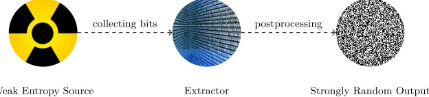
[Sun09], in contrast to pseudorandom generators which only expand some initial randomness using deterministic mathematical formulas. The design of a typical TRNG is illustrated inFigure 1below.

Weak Entropy Source Extractor Strongly Random Output collecting bits postprocessing

Fig. 1: True Random Number Generators. The scheme illustrates the typical design, where the building blocks are: (a) an entropy source (b) a harvesting mechanism and (c) a posprocessor (extractor).

Entropy Sources In practice, randomness can be gathered based on a physical phenomena (like radiation [hot], photons transmission, thermal noise [BP99], atmospheric noise [ran], jitters) or even from a human-device interaction (like timing events, keystrokes or mouse movements [pgp], shaking accelerators in mobile phones [VSH11] and other).

Extractors Extractors are functions which transform inputs of some required entropy amount into an almost uniform string of known length. To extract from every high-entropy source (that is, to have an extractor of general purpose), one needs to allow extractors to use small amount of auxiliary randomness, which can be “reinvested” as in the case of catalysts in chemistry. Also, one has to accept some small deviation of the output from being uniform (small enough to be acceptable for almost every application) and some entropy loss [RTS00]. Good extractors, simple, provable-secure and widely used in practice, are obtained from universal hash families [CW79]. We refer the reader to [Sha11] for a survey.

1.3 Entropy Estimating

In fact, one can extract randomness only if the given source distribution is close to a distribution of high min-entropy [RW04]. However, in order to avoid overes-timating security, we need to compute how much entropy we have; here Shannon entropy is much easier to estimate from samples than min-entropy1_{. In} particu-lar, this is the case of estimating entropy of data streams in an online manner, at low memory cost. Such estimators are an active research area and find im-portant applications in learning, data mining or network anomaly detection. The problem is that Shannon entropy overestimates crytpographic randomness, being much bigger than min-entropy.

Almost-Equivalence for Stateless Sources. A stateless source (called also memoryless) is a source which produces consecutive samples independently. While this is a restriction, it is often assumed by practitioners working on random number generators (cf. [LRSV12,BKMS09,BL05]) and argued to be reasonable for some classes of sources. An important result is obtained from a more general fact called Asymptotic Equipartition Property (AEP). Namelly, for a stateless source the Shannon entropy per bit is close to its min-entropy per bit.

A variant of the AEP:The min entropy per bit in a squenceX1, . . . , Xn

of i.id. samples fromX converges, whenn→ ∞, to the Shannon entropy ofX. More precisely

H∞(X1, . . . , Xn) n

in probability

−→ H(X) (1)

Thus, the AEP is a bridge connecting the heuristic use of Shannon entropy as a measure of extractable randomness (practice) and the provable security (extractors theory). The best known quantitative form appears in [Hol06].

Lemma 1 (Asymptotic Equipartition Property [Hol06]).LetX1, . . . , Xn

be i.i.d. samples from a distribution of Shannon entropyk. Then the distribution of(X1, . . . , Xn)is-close to a distribution of min entropykn−O

_p

log(1/)kn.

We can conclude that, up to an error of o(n), the number of extractable bits (very close to uniform) is at least as big as the Shannon entropy of (X1, . . . , Xn). But is it safe to assume (heuristically) that the equality (1) holds in practical parameter regimes?

1.4 Problem statement

We address the problem of finding upper bounds on the extraction rate.

Question: Suppose that we have a source which produces i.i.d samples

X1, X2, . . . each of Shannon entropy k. How much almost uniform bits can be extracted fromnsuch samples?

This question is well-motivated as no lower bounds toLemma 1 are known so far, and because of the popularity of the AEP herustic (1).

1

1.5 Our Result

The Tight No-Go Result We answer the posted question, showing that the convergence rate inEquation (1)given inLemma 1is optimal.

Theorem 1 (An Upper Bound on Bits Extractable from Shannon Sources).

In the above setting, we can extract no more that

N =kn−Θ(plog(1/)kn) (2)

bits which are -close (in the variation distance) to uniform. This matches the lower bound in [Hol06] (the constant underΘ(·)depends on the source X).

Corollary 1 (A Signifficant Entropy Loss in the AEP Heuristic Es-timate). In the above setting, the gap between the Shannon entropy and the number of extractable bits-close to uniform equals at least Θ(plog(1/)kn). In particular, for the recommended security level (= 2−80_{) we obtain the loss of} kn−N≈√80knbits, no matter what an extractor we use.

A Practical Example - How Not To Overestimate Security Imagine a mobile phone where the accelerometer is being used as an entropy source. Such a source was studied in [LPR11] and the Shannon entropy rate was estimated to be roughly 0.125 per bit. Since the recommended security level for almost random bits is= 2−80_{. According to the heuristic (1) we need roughly 128/0.125 = 1024}

samples to extract a 128-bit key. However taking into account the true error in ourTheorem 1we see that we need at leastn≈2214 bits!

1.6 Organization

InSection 2we give some basic facts and auxiliary technical results that will be used later. The proof of the main result, that isTheorem 1, is given in Section Section 3. Finally,Section 4concludes the work.

2

Preliminaries

2.1 Basic Definitions

The most popular way of measuring how two distributions are close is the sta-tistical distance.

Definition 1 (Statistical Distance). The statistical (or total variation) dis-tance of two distributionsX, Y is defined as

SD (X;Y) =X

x

|Pr[X =x]−Pr[Y =x]| (3)

Below we recall the definition of Shannon entropy and min entropy. The loga-rithms are taken at base 2.

Definition 2 (Shannon Entropy).The Shannon Entropy of a distributionX

equalsH(X) =−P

xPr[X =x] log Pr[X=x].

Definition 3 (Min Entropy). The min entropy of a distribution X equals

H∞(X) =−maxxlog Pr[X =x].

Definition 4 (Extractable Entropy, [RW04]). We say that X has k ex-tractable bits within distance , denoted H

ext(X) > k, if for some randomize

function Ext we have SD (Ext(X, S);Uk, S) ₆ , where Uk is a uniform k-bit string and S is an independent uniform string.

2.2 Technical Facts

Our proof uses the following characterization of “extractable” distributions.

Theorem 2 (An Upper Bound on Extractable Entropy, [RW04]). If

H

ext(X)>kthen X is-close toY such thatH∞(Y)>k.

The second important fact we use is the sharp bound on binomial tails.

Theorem 3 (Tight Binomial Tails [McK]). Let B(n, p) be a sum of inde-pendent Bernoulli trials with success probability p. Then for γ₆3₄qwe have

Pr [B(n, p)_>pn+γn] =Q

s

nγ2 pq

!

·ψ(p, q, n, γ) (4)

with the error term satisfies

ψ(p, q, n, γ) = exp _nγ2

2pq −nKL (p+γkp) +

1 2log

_p+γ

p ·

q q−γ

+Op,q

n−12

(5)

whereKL (akb) =alog(a/b) + (1−a) log((1−a)/(1−b)is the Kullback-Leibler divergence, and Qis the complement of the cumulative distribution function of the standard normal distribution.

3

Proof of

Theorem 1

3.1 Characterizing Extractable Entropy

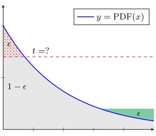
We state the following fact with an explanaition inFigure 2.

Lemma 2 (Lower bound on the extractable entropy).Let X be a distri-bution. Then for every distributionY which is-close to X, twe haveH∞(Y)6 −logt wheret satisfies

X

x

t=?

1−

y= PDF(x)

Fig. 2: The Entropy Smoothing Problem. For a given probability density func-tion, we want to cut a total mass of up toabove a possibly highest threshold (in dotted red) and rearrange it (in green), to keep the upper bound smallest possible.

The proof follows easily by observation that the optimal mass rearrangement (which maximizes H∞(Y)) is to decrease probability mass at biggest points. Without losing generality, we assume from now thatX ∈ {0,1} where Pr[X = 1] =p, q= 1−p. Define Xn_{= (X}

1, . . . , Xn). For anyx∈ {0,1}n we have

Pr[Xn =x] =pkxkqn−kxk. (7)

According to the last lemma andTheorem 2, we have

Hext (Xn)6−logt (8)

where

X

x

max (PXn(x)−t,0) =. (9)

From now we assume that

t=ppn+γnqqn−γn. (10)

3.2 Determining the Threshold t

The next key observation is thatt is actually small and can be ommitted. That is, we can simply cut the (1−)-quantile. This is stated in the lemma below.

Lemma 3 (Replacing the threshold by the quantile).Let x0∈ {0,1}n _be

a point such thatkx0k=pn+γn. Then we have

X

x: kxk>kx0k

max (PXn(x)−PXn(x0))>

1 2

X

x: kxk>kx0k

To prove the lemma, note that fromTheorem 3it follows that setting

γ0=γ+n−1log _p q (12) we obtain X

j>pn+γ0_n

_n j >3 4 · X

j>pn+γn

_n

j

(13)

when γ is sufficiently small comparing to pand q (formally this is justified by calculating the derivative with respect toγ and noticing that it is bigger by at most a factor of 1 + √γ

npq). But we also have

pjqn−j_>2·p(p+γ)nq(q−γ)n forj_>γ0n (14)

Therefore,

X

j>pn+γn

n j

pjqn−j_> X

j>pn+γ0_n

n j

pjqn−j

>2·p(p+γ)nq(q−γ)n· X

j>pn+γ0_n

_n

j

>2·3 4 ·p

(p+γ)n_q(q−γ)n_· X

j>pn+γn

_n

j

(15)

which finishes the proof.

3.3 Putting this all together

Now, by combiningLemma 2,Lemma 3and the estimateQ(x)≈x−1exp(−x2/2) forx0 we obtain

_>exp

−nKL (p+γkp)−log _nγ2

2pq

+Op,q(1)

(16)

which, because of the Taylor expansion KL (p+γkp) = _2pqγ2 +Op,q(γ3), gives us

γ_>Ω

s

log(1/)

pqn

!

(17)

4

Conclusion

We show an upper bound on the amount of random bits that can be extracted from a Shannon entropy source. Even in the most favorable case, that is for independent bits, the gap between the Shannon entropy and the amount of randomness that can be extracted is significant. In practical settings the Shannon entropy might be even 2 times bigger than the extractable entropy.

References

BKMS09. Jan Bouda, Jan Krhovjak, Vashek Matyas, and Petr Svenda,Towards true random number generation in mobile environments, NordSec 2009, Lecture Notes in Computer Science, vol. 5838, 2009, pp. 179–189.

BL05. Marco Bucci and Raimondo Luzzi,Design of testable random bit generators, CHES 2005, vol. 3659, 2005, pp. 147–156 (English).

BP99. Jun Benjamin and Kocher Paul,The intel random number generator, 1999. Cor99. Jean-Sebastien Coron,On the security of random sources, 1999.

CW79. J. L. Carter and M. N. Wegman,Universal classes of hash functions, Journal of Computer and System Sciences18(1979), no. 2, 143–154.

Hol06. Thomas Holenstein, Pseudorandom generators from one-way functions: A simple construction for any hardness, TCC 2006, Lecture Notes in Computer Science, vol. 3876, 2006, pp. 443–461.

hot. Hotbits project homepage,www.fourmilab.ch/hotbits/.

LPR11. C´edric Lauradoux, Julien Ponge, and Andrea R¨ock, Online Entropy Esti-mation for Non-Binary Sources and Applications on iPhone, Rapport de recherche, Inria, June 2011.

LRSV12. Patrick Lacharme, Andrea R¨ock, Vincent Strubel, and Marion Videau,The linux pseudorandom number generator revisited, Cryptology ePrint Archive, Report 2012/251, 2012,http://eprint.iacr.org/.

McK. Brendan D. McKay,ON LITTLEWOOD’S ESTIMATE FOR THE BINO-MIAL DISTRIBUTION, Advances in Applied Probability.

pgp. Pgp project homepage,http://www.pgpi.org. ran. Random.org project homepage,www.random.org.

RTS00. Jaikumar Radhakrishnan and Amnon Ta-Shma, Bounds for dispersers, extractors, and depth-two superconcentrators, SIAM JOURNAL ON DIS-CRETE MATHEMATICS13(2000), 2000.

RW04. R. Renner and S. Wolf,Smooth Renyi entropy and applications, ISIT 2004, 2004, p. 232.

Sha11. Ronen Shaltiel,An introduction to randomness extractors, ICALP’11, 2011, pp. 21–41.

Sun09. Berk Sunar, True random number generators for cryptography, Crypto-graphic Engineering (etinKaya Ko, ed.), Springer US, 2009, pp. 55–73 (En-glish).