Daniel J. Bernstein1,2, Andreas H¨ulsing2, Tanja Lange2, and Ruben Niederhagen2
1 Department of Computer Science University of Illinois at Chicago
Chicago, IL 60607–7045, USA [email protected]
2 Department of Mathematics and Computer Science Technische Universiteit Eindhoven
P.O. Box 513, 5600 MB Eindhoven, The Netherlands [email protected]
[email protected] [email protected]
Abstract. A 25-gigabyte “point obfuscation” challenge “using security parameter 60” was announced at the Crypto 2014 rump session; “point obfuscation” is another name for password hashing. This paper shows that the particular matrix-multiplication hash function used in the chal-lenge is much less secure than previous password-hashing functions are believed to be. This paper’s attack algorithm broke the challenge in just 19 minutes using a cluster of 21 PCs.
Keywords:symmetric cryptography, hash functions, password hashing, point obfuscation, matrix multiplication, in-the-middle attacks, meet-in-many-middles attacks
1
Introduction
Consider a server that knows a secret password11000101100100. The server could check an input password against this secret password using the following checkpassword algorithm (expressed in the Python language):
def checkpassword(input):
return int(input == "11000101100100")
But it is much better for the server to use the followingcheckpassword_hashed algorithm (see Appendix A for the definition of sha256hex):
def checkpassword_hashed(input): return int(sha256hex(input) == (
"ba0ab099c882de48c4156fc19c55762e" "83119f44b1d8401dba3745946a403a4f" ))
It is easy for the server to write down this checkpassword_hashed algorithm in the first place: apply SHA-256 to the secret password to obtain the string ba0...a4f, and then insert that string into a standardcheckpassword_hashed template. (Real servers normally store hashed passwords in a separate database, but in this paper we are not concerned with superficial distinctions between code and data.)
There is no reason to believe that these two algorithms compute identical functions. Presumably SHA-256 has a second (and third and so on) preimage of SHA-256(11000101100100), i.e., a string for which checkpassword_hashed re-turns 1 whilecheckpassword returns 0. However, finding any such string would be a huge advance in SHA-256 cryptanalysis. The checkpassword_hashed al-gorithm outputs 1 for input 11000101100100, just like checkpassword, and outputs 0 for all other inputs that have been tried, just like checkpassword.
The core advantage ofcheckpassword_hashedover checkpasswordis that it isobfuscated. If thecheckpasswordalgorithm is leaked to an attacker then the attacker immediately sees the secret password and seizes control of all resources protected by that password. If checkpassword_hashed is leaked to an attacker then the attacker still does not see the secret password without solving a SHA-256 preimage problem: the loss of confidentiality does not immediately create a loss of integrity.
Obfuscation is a broad concept. There are many aspects of programs that one might wish to obfuscate and that are not obfuscated incheckpassword_hashed: for example, one can immediately see that the program is carrying out a SHA-256 computation, and that (unless SHA-SHA-256 is weak) there are very few short inputs for which the program prints 1. In the terminology of some recent papers (see Section 2), what is obfuscated here is the key in a particular family of “keyed functions”, but not the choice of family. Further comments on general obfuscation appear below. We emphasize password obfuscation because it is an important special case: a widely deployed application using widely studied symmetric techniques.
secret password is a string of 14 digits, each 0 or 1, then the attacker can simply try hashing all 214 possibilities for that string. Even worse, if the attacker sees many checkpassword_hashed algorithms from many users’ secret passwords, the attacker can efficiently compare all of them to this database of 214 hashes: the cost of multiple-target preimage attacks is essentially linear in the sum of the number of targets and the number of guesses, rather than the product.
There are three standard responses to these problems. First, to eliminate the multiple-target problem, the server randomizes the hashing. For example, the server might store the same secret password 11000101100100 as the following checkpassword_hashed_saltedalgorithm, whereprefix was chosen randomly by the server for storing this password:
def checkpassword_hashed_salted(input):
prefix = "b1884428881e20fe61c7629a0f71fcda" return int(sha256hex(prefix + input) == (
"5f5616075f77375f1e36e2b707e55744" "91a308c39653afe689b7a958455e65d2" ))
The attacker sees the prefix and can still find this password using at most 214 guesses, but the attacker can no longer share work across multiple targets. (This benefit does not rely on randomness: any non-repeating prefix is adequate. For example, the prefix can be chosen as a counter; on the other hand, this requires maintaining state and raises questions of what information is leaked by the counter.)
Second, the server chooses a hash function that is much more expensive than SHA-256, multiplying the server’s cost by some factor F but also multiplying the attack cost by almost exactly F, if the hash function is designed well. The ongoing “Password Hashing Competition” [9] has received dozens of submissions of “memory-hard” hash functions that are designed to be expensive to compute even for an attacker manufacturing special-purpose chips to attack those partic-ular functions.
Third, users are encouraged to choose passwords from a much larger space. A password having only 14 bits of entropy is highly substandard: for example, the recent paper [14] reports techniques for users to memorize passwords with four times as much entropy.
1.2. Matrix-multiplication password hashing: the “point obfuscation” challenge. A “point obfuscation” challenge was announced by Apon, Huang, Katz, and Malozemoff [7] at the Crypto 2014 rump session. “Point obfuscation” is the same concept as password hashing: see, e.g., [33] (a hashed password is a “provably secure obfuscation of a ‘point function’ under the random oracle model”).
is to determine the secret 14-bit input: “learn the point and you win!” An ac-companying October 2014 paper [5] described the challenge as having “security parameter 60”, where “security parameterλis designed to bound the probability of successful attacks by 2−λ”.
We tried the 25-gigabyte program on a PC with the following relevant re-sources: an 8-core 125-watt AMD FX-8350 “Piledriver” CPU (about $200), 32 gigabytes of RAM (about $400), and a 2-terabyte hard drive (about $100). The program took slightly over 4 hours for a single input. A brute-force attack using this program would obviously have been feasible but would have taken over 65536 hours worst-case and over 32768 hours on average, i.e., an average of nearly 4 years on the same PC, consuming 500 watt-years of electricity.
1.3. Attacking matrix-multiplication password hashing.In this paper we explain how we solved the same challenge in just 19 minutes using a cluster of 21 such PCs. The solution is 11000101100100; we reused this string above as our example of a secret password. Of course, knowing this solution allowed us to compress the original program to a much fastercheckpassword algorithm.
The time for our attack algorithm against a worst-case input point would have been just 34 minutes, about 5000 times faster than the original brute-force attack, using under 0.2 watt-years of electricity. Our current software is slightly faster: it uses just 29.5 minutes on 22 PCs, or 35.7 minutes on 16 PCs.
More generally, for an n-bit point function obfuscated in the same way, our attack algorithm is asymptotically n4/2 times faster than a brute-force search using the original program. This quartic speedup combines four linear speedups explained in this paper, taking advantage of the matrix-multiplication structure of the obfuscated program. Two of the four speedups (Section 3) are applicable to individual inputs, and could have been integrated into the original program, preserving the ratio between attack time and evaluation time; but the other two speedups (Section 4) share work between separate inputs, making the attack much faster than a simple brute-force attack.
See Section 1.6 for generalizations to more functions.
1.4. Matrix-multiplication password hashing vs. state-of-the-art pass-word hashing.It is well known that a 2n-guess preimage attack against a hash function, cipher, etc. does not costexactly 2n times as much as a single function evaluation: there are always ways to merge small amounts of initial work across multiple inputs, and to skip small amounts of final work. See, for example, [34] (“Reduce the DES encryption from 16 rounds to the equivalent of ≈9.5 rounds, by shortcircuit evaluation and early aborts”), [29] (“biclique” attacks against various hash functions), and [13] (“biclique” attacks against AES).
Even worse, the matrix-multiplication approach has severe performance prob-lems that end up limiting the number n of input bits. The “obfuscated point function” includes 2nmatrices, each matrix havingn+2 rows andn+2 columns, each entry having approximately 4((λ + 1)(n+ 4) + 2)2log2λ bits; recall that λ is the target “security parameter”. If λ is just 60 and n is above 36 then a single obfuscated password does not fit on a 2-terabyte hard drive, never mind the time and memory required to print and evaluate the function.
Earlier password-hashing functions handle a practically unlimited number of input bits with negligible slowdowns; fit obfuscated passwords into far fewer bits (a small constant times the target security level); allow the user far more flexibility to select the amount of time and memory used to check a password; and do not have the worrisome matrix structure exploited by our attacks.
1.5. Context: obfuscating other functions. Why, given the extensive hash-ing literature, would anyone introduce a new password-obfuscation method with unnecessary mathematical structure, obvious performance problems, and no ob-vious advantages? To answer this question, we now explain the context that led to the Apon–Huang–Katz–Malozemoff point-obfuscation challenge; we start by emphasizing that their goal was not to introduce a new point-obfuscation method.
Point functions are not the only functions that cryptographers obfuscate. Consider, for example, the following fast algorithm to compute the pqth power of an input mod pq, where p and q are particular prime numbers shown in the algorithm:
def rsa_encrypt_unobfuscated(x):
p = 37975227936943673922808872755445627854565536638199 q = 40094690950920881030683735292761468389214899724061 pinv = 23636949109494599360568667562368545559934804514793 qinv = 15587761943858646484534622935500804086684608227153 return (qinv*q*pow(x,q,p) + pinv*p*pow(x,p,q)) % (p*q)
The following algorithm is not as fast but uses only the product pq: def rsa_encrypt(x):
pq = int("15226050279225333605356183781326374297180681149613" "80688657908494580122963258952897654000350692006139") return pow(x,pq,pq)
These algorithms compute exactly the same function x 7→ xpq modpq, but the primespandqare exposed inrsa_encrypt_unobfuscatedwhile they are obfus-cated inrsa_encrypt. This obfuscation is exactly the reason that rsa_encrypt is safe to publish. In other words, RSA public-key encryption is an obfuscation of a secret-key encryption scheme.
In a FOCS 2013 paper [25], Garg, Gentry, Halevi, Raykova, Sahai, and Waters proposed an obfuscation method that takes any fast algorithm A as input and “efficiently” produces an obfuscated algorithm Obf(A). The security goal for Obf is to be an “indistinguishability obfuscator”: this means that Obf(A) is indistinguishable from Obf(A0) if A and A0 are fast algorithms computing the same function.
For example, if Obf is an indistinguishability obfuscator, and if an attacker can extract p and q from Obf(rsa_encrypt_unobfuscated), then the attacker can also extract p and q from Obf(rsa_encrypt), since the two obfuscations are in-distinguishable; so the attacker can “efficiently” extractpandq from pq, by first computing Obf(rsa_encrypt). Contrapositive: if Obf is an indistinguishability obfuscator and the attacker cannot “efficiently” extract p and q from pq, then the attacker cannot extract p and q from Obf(rsa_encrypt_unobfuscated); i.e., Obf(rsa_encrypt_unobfuscated) hides p and q at least as effectively as rsa_encryptdoes.
Another example, returning to symmetric cryptography: It is reasonable to as-sume thatcheckpasswordandcheckpassword_hashedcompute the same func-tion if the input length is restricted to, e.g., 200 bits. This assumpfunc-tion, together with the assumption that Obf is an indistinguishability obfuscator, implies that Obf(checkpassword) hides a ≤200-bit secret password at least as effectively as checkpassword_hashed does.
These examples illustrate the generality of indistinguishability obfuscation. In the words of Goldwasser and Rothblum [27], efficient indistinguishability obfus-cation is “best-possible obfusobfus-cation”, hiding everything that ad-hoc techniques would be able to hide.
There are, however, two critical caveats. First, it is not at all clear that the Obf proposal from [25] (or any newer proposal) will survive cryptanalysis. There are actually two alternative proposals in [25]: the first relies on multilinear maps [24] from Garg, Gentry, and Halevi, and the second relies on multilinear maps [22] from Coron, Lepoint, and Tibouchi. In a paper [19] posted early November 2014 (a week after we announced our solution to the “point obfuscation” challenge), Cheon, Han, Lee, Ryu, and Stehl´e announced a complete break of the main security assumption in [22], undermining a remarkable number of papers built on top of [22]. The attack from [19] does not seem to break the application of [22] to point obfuscation (since “encodings of zero” are not provided in this context), but it illustrates the importance of leaving adequate time for cryptanalysis. A followup work by Gentry, Halevi, Maji, and Sahai [26] extends the attack from [19] to some settings where no “encodings of zero” below the “maximal level” are available, although the authors of [26] state that “so far we do not have a working attack on current obfuscation candidates”.
functions where the previous techniques apply. We would expect the generality of these proposals to damage the security-performance curve in a broad range of real applications covered by the previous techniques, implying that these proposals should be used only for applications outside that range.
The goal of Apon, Huang, Katz, and Malozemoff was to investigate “the prac-ticality of cryptographic program obfuscation”. Their obfuscator is not limited to point functions; it takes more general circuits as input. However, after per-formance evaluation, they concluded that “program obfuscation is still far from being deployable, with the most complex functionality we are able to obfuscate being a 16-bit point function”; see [5, page 2]. They chose a 14-bit point function as a challenge.
1.6. Attacking matrix-multiplication-based obfuscation of any func-tion. The real-world importance of password hashing justifies focusing on point functions, but we have also adapted our attack algorithm to arbitrary n-bit-to-1-bit functions. Specifically, we have considered the method explained in [5] to obfuscate an arbitraryn-bit-to-1-bit function, and adapted our attack algorithm to this level of generality. For the general case, with u pairs of w×w matrices using n input bits, we save a factor of roughly uw/2 in evaluating each input, and a further factor of approximately n/log2w in evaluating all inputs. The n/log2w increases to n/2 for the standard input-bit order described in [5], but for an arbitrary input-bit order our attack is still considerably faster than a simple brute-force attack. See Section 8.
We comment that standard cryptographic hashing can be used to obfuscate general functions. We suggest the following trivial obfuscation technique as a baseline for future obfuscation challenges: precompute a table of hashes of the inputs that produce 1; add fake random hashes to pad the table to size 2n (or a smaller sizeT, if it is acceptable to reveal that at mostT inputs produce 1); and sort the table for fast lookups. This does not take polynomial time as n → ∞ (forT = 2n), but it nevertheless appears to be smaller, faster, and stronger than all of the recently proposed matrix-multiplication-based obfuscation techniques for every feasible value of n.
2
Review of the obfuscation scheme
applying the same attack strategy with the Garg–Gentry–Halevi [24] multilinear map in place of CLT.
Most of the Obf literature does not state concrete parameters and does not present computer-verified examples. The first implementations, first examples, and first challenge were from Apon, Huang, Katz, and Malozemoff in [5], [6], and [7], providing an important foundation for quantifying and verifying attack performance.
The challenge given in [5] is an obfuscation of a point function, so we first give a self-contained description of these obfuscated point-function programs from the attacker’s perspective; we then comment briefly on more general functions. For details on how the matrices below are constructed, we refer the reader to [4], [22], and of course [5]; but these details are not relevant to our attack.
2.1. Obfuscated point functions. A point function is a function on {0,1}n that returns 1 for exactly one secret vector of length n and 0 otherwise. The obfuscation scheme starts with this secret vector and an additional security parameter λ related to the security of the multilinear map.
The obfuscated version of the point function is given by a list of 2n public (n+ 2)×(n+ 2) matrices Bb,k for 1≤b≤nandk ∈ {0,1} with integer entries; a row vector s of length n+ 2 with integer entries; a column vector t of length n+ 2 with integer entries; an integerpzt (a “zero test” value, not to be confused with an “encoding of zero”); and a positive integer q. All of the entries and pzt are between 0 and q−1 and appear random. The number of bits of q has an essentially linear impact upon our attack cost; [5] chooses the number of bits of q to be approximately 4((λ+ 1)(n+ 4) + 2)2log2λ for multilinear-map security reasons.
The obfuscated program works as follows:
• Take as input an n-bit vector x= (x[1], x[2], . . . , x[n]).
• Compute the integer matrix A = B1,x[1]B2,x[2]· · ·Bn,x[n] by successive ma-trix multiplications.
• Compute the integery(x) =sAtby a vector-matrix multiplication and a dot product.
• Compute y(x)pzt and reduce mod q to the range [−(q−1)/2,(q−1)/2]. • Multiply the remainder by 22λ+11, divide by q, and round to the nearest
integer. This result is by definition the matrix-multiplication hash of x. • Output 0 if this hash is 0; output 1 otherwise.
We have confirmed these steps against the software in [6].
2.2. Initial security analysis.A straightforward brute-force attack determines the secret vector by computing the matrix-multiplication hash of all 2n vectors x. Of course, the computation stops once a correct hash is found.
Unfortunately [5] and [7] do not include timings for λ = 60 and n = 14, so we timed the software from [6] on one of our PCs and saw that each evaluation took 245 minutes, i.e., 245.74 cycles at 4GHz. As the code automatically used all 8 cores of the CPU, this leads to a total of 248.74 cycles per evaluation. A brute-force computation using this software would take 214 ·248.74 = 262.74 cycles worst-case, and would take more than 260 cycles for 85% of all inputs. For comparison, recall that the CLT parameters were designed to just barely provide 2λ = 260 security, although the time scale for the 260 here is not clear. If the time scale of the security parameter is close to one cycle then the cost of these two attacks is balanced.
In their Crypto 2014 rump-session announcement [8], the authors declared this brute-force attack to be infeasible: “The great part is, it’s only 14 bits, so you think you can try all 2 to the 14 points, but it takes so long to evaluate that it’s not feasible.” The authors concluded in [5, Section 5] that they were “able to obfuscate some ‘meaningful’ programs” and that “it is important to note that the fact that we can produce any ‘useful’ obfuscations at all is surprising”.
We agree that a 500-watt-year computation is a nonnegligible investment of computer time (although we would not characterize it as “infeasible”). However, in Section 3 we show how to make evaluation two orders of magnitude faster, bringing a brute-force attack within reach of a small computer cluster in a matter of days. Furthermore, in Section 4 we present a meet-in-the-middle attack that is another two orders of magnitude faster.
2.3. Obfuscation of general functions and keyed functions.The obfusca-tion scheme in [4] transforms any function into a sequence of matrix multiplica-tions. At every multiplication the matrix is selected based on a bit of the input xbut usually the bits ofx are used multiple times. For general circuits of length ` the paper constructs an oblivious relaxed matrix branching program of length n`which cycles ` times through thenentries of xin sequence to select from 2n` matrices. In that case most of the matrices are obfuscated identity matrices but the regular access pattern stops the attacker from learning anything about the function.
Sometimes (as in the password-hashing example) the structure of the circuit is already public, and all that one wants to obfuscate is a secret key. In other words, the circuit computes fz(x) = φ(z, x) for some secret key z, where φ is a publicly known branching program; the obfuscation needs to protect only the secret keyz, and does not need to hide the functionφ. This is called “obfuscation of keyed functions” in [4]. For this class of functions the length of the obfuscated program equals the length of the circuit forφ; the bits ofx are used (and reused as often as necessary) in a public order determined by φ.
3
Faster algorithms for one input
This section describes two speedups to the obfuscated programs described in Section 2. These speedups are important for constructive as well as destructive applications.
Combining these two ideas reduced our time to evaluate the obfuscated point function for a single input from 245 minutes to under 5 minutes (4 minutes 51 seconds), both measured on the same 8-core CPU. The authors of [6] have recently included these speedups in their software, with credit to us.
3.1. Cost analysis for the original algorithm.Schoolbook multiplication of the two (n+ 2)×(n+ 2) matricesB1,x[1] andB2,x[2] uses (n+ 2)3 multiplications of matrix entries. Similar comments apply to all n−1 matrix multiplications, for a total of (n−1)(n+ 2)3 multiplications of matrix entries.
This quartic operation count understates the asymptotic complexity of the algorithm for two reasons, even when the security parameter λ is treated as a constant. The first reason is that the number of bits of q grows quadratically withn. The second reason is that the entries inB1,x[1]B2,x[2] have about twice as many bits as the entries in the original matrices, the entries inB1,x[1]B2,x[2]B3,x[3] have about three times as many bits, etc. The paper [5] reports timings for point functions withn∈ {8,12,16}for security parameter 52, and in particular reports microbenchmarks of the time taken for each of the matrix products, starting with the first; these microbenchmarks clearly show the slowdown from one product to the next, and the paper explains that “each multiplication increases the mul-tilinearity level of the underlying graded encoding scheme and thus the size of the resulting encoding”.
We now account for the size of the matrix entries. Recall that state-of-the-art multiplication techniques (see, e.g., [11]) take time essentially linear in b, i.e., b1+o(1), to multiply b-bit integers. The original entries have size quadratic in n, and the products quickly grow to size cubic inn. More precisely, the final product A = B1,x[1]· · ·Bn,x[n] has entries bounded by (n+ 2)n−1(q−1)n and typically larger than (q−1)n; similar bounds apply to intermediate products. More than n/2 of the products have typical entries above (q−1)n/2, so the multiplication time is dominated by integers having size cubic in n.
The total time to computeA is n7+o(1) for constant λ, equivalent to n5+o(1) multiplications of integers on the scale of q. This time dominates the total time for the algorithm.
State-of-the-art division techniques take time within a constant factor of state-of-the-art multiplication techniques, so (n+ 2)2 reductions mod q take asymp-totically negligible time compared to (n+ 2)3 multiplications. The number of bits in each intermediate integer drops from cubic in nto quadratic in n.
More precisely, the asymptotic speedup factor isn/2, since the original multi-plication inputs had on average aboutn/2 times as many bits asq. We observe a smaller speedup factor for concrete values ofn, mainly because of the overhead for the extra divisions.
The total time to compute A modq is n6+o(1) for constant λ, dominated by (n−1)(n+ 2)3 = n4 + 5n3+ 6n2−4n−8 multiplications of integers bounded by q, inside (n−1)(n+ 2)2 =n3+ 3n2−4 dot products modq.
3.3. Matrix-vector multiplications.We further improve the computation by reordering the operations used to compute y(x): specifically, instead of comput-ing A, we compute
y(x) = · · · (sB1,x[1])B2,x[2]
· · ·Bn,x[n]
t.
This sequence of operations requiresnmatrix products and a final vector-vector multiplication.
This combines straightforwardly with intermediate reductions modqas above. The total time to compute y(x) modq is n5+o(1), dominated by n(n+ 2) + 1 = (n+ 1)2 dot products modq.
4
Faster algorithms for many inputs
A brute-force attack iterates through the whole input range and computes the evaluation for each possible input until the result of the evaluation is 1 and thus the correct input has been found. In terms of complexity our improvements from Section 3 reduced the cost of brute-forcing an n-bit point function from time n7+o(1)2n to time n5+o(1)2n for constant λ, dominated by (n+ 1)22n dot products mod q. This algorithm is displayed in Figure 4.1.
This section presents further reductions to the complexity of the attack. These share computations between evaluations of many inputs and have no matching speedups on the constructive side (which usually only evaluates at a single point at once and in any case cannot be expected to have related inputs).
4.2. Reusing intermediate products.Recall that Section 3 computesy(x) = sB1,x[1]· · ·Bn,x[n]t mod q by multiplying from left to right: the last two steps are to multiply the vector sB1,x[1]· · ·Bn−1,x[n−1] by Bn,x[n] and then by t.
Notice that this vector does not depend on the choice ofx[n]. By computing this vector, multiplying the vector by Bn,0 and then by t, and multiplying the same vector by Bn,1 and then by t, we obtain both y(x[1], . . . , x[n−1],0) and y(x[1], . . . , x[n−1],1). This saves almost half of the cost of the computation.
execfile(’subroutines.py’) import itertools
def bruteforce():
for x in itertools.product([0,1],repeat=n): L = s
for b in range(n):
L = [dot(L,[B[b][x[b]][i * w + j] for j in range(w)]) for i in range(w)]
result = solution(x,dot(L,t)) if result: return result
print bruteforce()
Fig. 4.1. Brute-force attack algorithm, separately evaluating y(x) modq for each x, including the speedups of Section 3: reducing intermediate matrix products mod q
(inside dot) and replacing matrix-matrix products with vector-matrix products. See Appendix A for definitions of subroutines.
final multiplications byt, for a total of (n+2)(2n+1−2)+2n = (2n+5)2n−2(n+2) dot products modq.
To minimize memory requirements, we enumerate x in lexicographic order, maintaining a stack of intermediate products. We reuse products on the stack to the extent allowed by the common prefix between x and the previous x. In most cases this common prefix is almost the entire stack. On average slightly fewer than two matrix-vector products need to be recomputed for each x. See Figure 4.3 for a recursive version of this algorithm.
4.4. A meet-in-the-middle attack. To do better we change the order of matrix multiplication yet again, separating ` “left” bits from n−` “right” bits:
y(x) = (sB1,x[1]· · ·B`,x[`])(B`+1,x[`+1]· · ·Bn,x[n]t).
We exploit this separation to store and reuse some computations. Specifically, we precompute a table of “left” products
L[x[1], . . . , x[`]] =sB1,x[1]· · ·B`,x[`]
for all 2` choices of (x[1], . . . , x[`]). The main computation of all y(x) works as follows: for each choice of (x[`+ 1], . . . , x[n]), compute the “right” product
R[x[`+ 1], . . . , x[n]] =B`+1,x[`+1]· · ·Bn,x[n]t, and then multiply each element of the L table by this vector.
execfile(’subroutines.py’)
def reuseproducts(xleft,L): b = len(xleft)
if b == n: return solution(xleft,dot(L,t)) for xb in [0,1]:
newL = [dot(L,[B[b][xb][i * w + j] for j in range(w)]) for i in range(w)]
result = reuseproducts(xleft + [xb],newL) if result: return result
print reuseproducts([],s)
Fig. 4.3.Attack algorithm sharing computations of intermediate products across many inputs x.
Computing a single right product B`+1,x[`+1]· · ·Bn,x[n]t from right to left (starting fromt) takesn−` matrix-vector products, for a total of (n−`)(n+ 2) dot products mod q. The outer loop in the main computation therefore uses (n−`)(n+ 2)2n−` dot products mod q in the worst case. The inner loop in the main computation, computing all y(x), uses just 2n dot products mod q in total in the worst case.
The total number of dot products modq in this algorithm, including precom-putation, is`(n+2)2`+(n−`)(n+2)2n−`+2n. In particular, for`=n/2 (assum-ingnis even), the number of dot products modq simplifies ton(n+ 2)2n/2+ 2n. For a traditional meet-in-the-middle attack, the outer loop of the main com-putation simply looks up each result in a precomputed sorted table. Our notion of “meet” is more complicated, and requires inspecting each element of the table, but this is still a considerable speedup: each inspection is simply a dot product, much faster than the vector-matrix multiplications used before.
We comment that taking`logarithmic innproduces almost the same speedup with polynomial memory consumption. More precisely, taking ` close to 2 log2n means that 2n−` is smaller than 2n by a factor roughly n2, so the term (n− `)(n+ 2)2n−` is on the same scale as 2n. The table then contains roughly n2 vectors, similar size to the original 2nmatrices. Taking slightly larger ` reduces the term (n−`)(n+ 2)2n−` to a smaller scale. A similar choice of ` becomes important for speed in Section 8.2.
4.5. Combining the ideas.One can easily reuse intermediate products in the meet-in-the-middle attack. See Figure 4.6. This reduces the precomputation to 2`+1−2 vector-matrix multiplications, i.e., (n+ 2)(2`+1−2) dot products modq. It similarly reduces the outer loop of the main computation to (n+2)(2n−`+1−2) dot products modq.
execfile(’subroutines.py’)
l = n // 2
def precompute(xleft,L): b = len(xleft)
if b == l: return [(xleft,L)] result = []
for xb in [0,1]:
newL = [dot(L,[B[b][xb][i * w + j] for j in range(w)]) for i in range(w)]
result += precompute(xleft + [xb],newL) return result
table = precompute([],s)
def mainloop(xright,R): b = len(xright)
if b == n - l:
for xleft,L in table:
result = solution(xleft + xright,dot(L,R)) if result: return result
return
for xb in [0,1]:
newR = [dot(R,[B[n - 1 - b][xb][j * w + i] for j in range(w)]) for i in range(w)]
result = mainloop([xb] + xright,newR) if result: return result
print mainloop([],t)
Fig. 4.6. Meet-in-the-middle attack algorithm, including reuse of intermediate prod-ucts, using`=bn/2c bits on the left andn−` bits on the right.
This is not much smaller than the meet-in-the-middle attack without reuse: the dominant term is the same 2n. However, as above one can take much smaller ` to reduce memory consumption. The reuse now allows ` to be taken almost as small as log2n without significantly compromising speed, so the precomputed table is now much smaller than the original 2n matrices.
to Shanks’s “baby-step giant-step” discrete-logarithm method. Compare [37, pages 419–420] to [35, page 439, top].
5
Parallelization
We implemented our attack for shared-memory systems using OpenMP and for cluster systems using MPI. In general, brute-force attacks are embarrassingly parallel, i.e., the search space can be distributed over the computing nodes with-out any need for communication, resulting in a perfectly scalable parallelization. However, for this attack, some computations are shared between consecutive it-erations. Therefore, some cooperation and communication are required between computing nodes.
5.1. Precomputation. Recall that the precomputation step computes all 2` possible cases for the “left” ` bits of the whole input space. A non-parallel implementation first computes ` vector-matrix multiplications for sB1,0· · ·B`,0 and stores the first`−1 intermediate products on a stack. As many intermediate products as possible are reused for each subsequent case.
For a shared-memory system, all data can be shared between the threads. Furthermore, the vector-matrix multiplications expose a sufficient amount of parallelism such that the threads can cooperate on the computation of each multiplication. There is some loss in parallel efficiency due to the need for syn-chronization and work-share imbalance.
For a cluster system, communication and synchronization of such a workload distribution would be too expensive. Therefore, we split the input range for the precomputation between the cluster nodes, compute each section of the precom-puted table independently, and finally broadcast the table entries to all cluster nodes. For simplicity, we split the input range evenly which results in some work-load imbalance. (On each node, the workwork-load is distributed as described above over several threads to use all CPU cores on each node.) This procedure has some loss in parallel efficiency due to the fact that each cluster node separately per-forms k vector-matrix multiplications for the first precomputation in its range, due to some workload imbalance, and due to the final all-to-all communication.
5.2. Main computation. For simplicity, we start the main computation once the whole precomputed table L is available. Recall that a non-parallel imple-mentation of the main computation first computes the vector R[0, . . . ,0] = B`+1,0· · ·Bn,0t using n− ` matrix-vector multiplications, and multiplies this vector by all 2` table entries. It then moves to other possibilities for the “right” n−` bits, reusing intermediate products in a similar way to the precomputation and multiplying each resulting vectorR[. . .] by all 2` table entries.
parallelization of precomputation, there is some loss of parallel efficiency due to synchronization and work-share imbalance for the vector-matrix multiplications and some loss due to work-share imbalance for the vector-vector multiplications. For a cluster system we again cannot efficiently distribute the workload of one vector-matrix multiplication over several cluster nodes. Therefore, we distribute the search space evenly over the cluster nodes and let each cluster node compute its share of the workload independently. This approach creates some redundant work because each cluster node computes its own initialR[. . .] usingn−` matrix-vector multiplications.
6
Performance measurements
We used 22 PCs in the Saber cluster [12] for the attack. Each PC is of the type described earlier, including an 8-core CPU. The PCs are connected by a gigabit Ethernet network. Each PC also has two GK110 GPUs but we did not use these GPUs.
6.1. First break of the challenge.We implemented the single-input optimiza-tions described in Section 3 and used 20 PCs to compute 214 point evaluations for all possible inputs. This revealed the secret point 11000101100100 after about 23 hours. The worst-case runtime for this approach on these 20 PCs is about 52 hours for checking all 214 possible input points. On 18 October 2014 we sent the authors of [5] the solution to the challenge, and a few hours later they confirmed that the solution was correct.
6.2. Second break of the challenge.We implemented the multiple-input op-timizations described in Section 4 and the parallelization described in Section 5. Our optimized attack implementation found the input point in under 19 minutes on 21 PCs; this includes the time to precompute a tableLof size 27. The worst-case runtime of the attack for checking all 214 possible input points is under 34 minutes on 21 PCs.
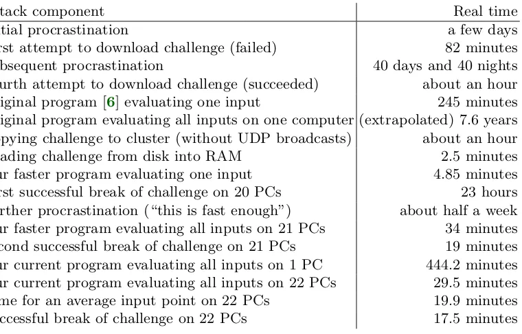
6.3. Additional latency. Obviously “19 minutes” understates the real time that elapsed between the announcement of the challenge (19 August 2014) and our solution of the challenge with our second program (25 October 2014). See Table 6.4 for a broader perspective.
The largest deterrent was the difficulty of downloading 25 gigabytes. When-ever a connection broke, the server would insist on starting from the beginning (“HTTP server doesn’t seem to support byte ranges”), presumably because the server stores all files in a compressed format that does not support random access. The same restriction also meant that we could not download different portions of the file in parallel.
Attack component Real time
Initial procrastination a few days
First attempt to download challenge (failed) 82 minutes Subsequent procrastination 40 days and 40 nights Fourth attempt to download challenge (succeeded) about an hour Original program [6] evaluating one input 245 minutes Original program evaluating all inputs on one computer (extrapolated) 7.6 years Copying challenge to cluster (without UDP broadcasts) about an hour Reading challenge from disk into RAM 2.5 minutes Our faster program evaluating one input 4.85 minutes First successful break of challenge on 20 PCs 23 hours Further procrastination (“this is fast enough”) about half a week Our faster program evaluating all inputs on 21 PCs 34 minutes Second successful break of challenge on 21 PCs 19 minutes Our current program evaluating all inputs on 1 PC 444.2 minutes Our current program evaluating all inputs on 22 PCs 29.5 minutes Time for an average input point on 22 PCs 19.9 minutes Successful break of challenge on 22 PCs 17.5 minutes
Table 6.4. Measurements of real time actually consumed by various components of complete attack, starting from announcement of challenge.
instead of an L table: the portion of the input relevant to L is available sooner than the portion of the input relevant to R.
6.5. Timings of various software components. We have put the latest version of our software online athttp://obviouscation.cr.yp.to. We applied this software to the same challenge on 22 PCs. The software took a total time of 1769 seconds (29.5 minutes) to check all 214 input points. An average input point was checked within 1191 seconds (19.9 minutes). The secret challenge point was found within 1048 seconds (17.5 minutes).
The rest of this section describes the time taken by various components of this computation.
Each vector-matrix multiplication took 15.577 s on average (15.091 minimum, 16.421 maximum), using all eight cores jointly. For comparison, on a single core, a vector-matrix multiplication requires about 115 s. Therefore, we achieve a par-allel efficiency of 15115.577s/8s ≈92% for parallel vector-matrix multiplication.
Each y computation took 8.986 s on average (7.975 minimum, 9.820 maxi-mum), using a single core. Each y computation consists of one vector-vector multiplication, one multiplication by pzt (which we could absorb into the pre-computed table, producing a small speedup), and one reduction mod q.
On a single machine (no MPI parallelization), after a reboot to flush the challenge from RAM, the timing breaks down as follows:
(a) Computing the first ` = 7 vector-matrix products: 107.623 s. 4. Loading the matrices for “right” bit positions: 78.490 s.
5. Total computation of all 214 evaluations: 22518.900 s.
(a) Computing the first n−` = 7 matrix-vector products: 109.731 s.
Overall total runtime: 26654 s (444.2 minutes). From these computations, steps 1, 2a, 4, and 5a are not parallelized for cluster computation. The total timing breakdown on 22 PCs, after a reboot of all PCs, is as follows:
1. Loading the matrices for “left” bit positions: 89.449 s average (75.786 on the fastest node, 104.696 on the slowest node). With more effort we could have overlapped most of this loading (and the subsequent loading) with computation, or skipped all disk copies by keeping the matrices in RAM. 2. Total precomputation of 27 = 128 table entries: 253.346 s average (217.893
minimum, 295.999 maximum).
(a) Computing the first ` = 7 vector-matrix products: 107.951 s average (107.173 minimum, 109.297 maximum).
3. All-to-all communication: 153.591 s average (100.848 minimum, 199.200 max-imum); i.e., about 53 s average idle time for the busier nodes to catch up, followed by about 101 s of communication. With more effort we could have overlapped most of this communication with computation.
4. Loading the matrices for “right” bit positions: 85.412 s average (73.710 min-imum, 97.526 maximum).
5. Total computation of all 214 evaluations: 1097.680 s average (942.981 mini-mum, 1169.520 maximum).
(a) Computing the firstn−`= 7 matrix-vector products: 108.878 s average (107.713 minimum, 110.001 maximum).
6. Final idle time waiting for all other nodes to finish computation: 80.277 s average (0.076 minimum, 80.277 maximum).
Overall total runtime, including MPI startup overhead: 1769 s (29.5 minutes). The overall parallel efficiency of the cluster parallelization thus is 26654 s1769 s/22 ≈ 68%. Steps 1, 2a, 3, 4, and 5a, totaling 545.281 s, are those parts of the com-putation that contain parallelization overhead (in particular the communica-tion time in step 3 is added compared to the single-machine case). Remov-ing these steps from the efficiency calculation results in a parallel efficiency of
(26654 s−380 s)/22
1769 s−545 s ≈98%, which shows that those steps are responsible for almost all of the loss in parallel efficiency.
7
Further speedups
7.1. Reusing transforms. One fast way to compute an m-coefficient product of two univariate polynomials is to evaluate each polynomial at the mth roots of 1 (assuming that there is a primitive mth root of 1 in the coefficient ring), multiply the values, and interpolate the product polynomial from the products of values. The evaluation and interpolation take only Θ(mlog2m) arithmetic operations using a standard radix-2 FFT (assuming thatmis a power of 2), and multiplying values takes only m arithmetic operations.
More generally, to multiply two w×w matrices of polynomials where each entry of the output is known to fit intomcoefficients, one can evaluate each poly-nomial at themth roots of 1, multiply the matrices of values, and interpolate the product matrix. Note that intermediate values are computed in the evaluation domain; interpolation is postponed until the end of the matrix multiplication. The evaluation takes only Θ(w2mlog
2m) arithmetic operations; schoolbook multiplication of the resulting matrices of values takes onlyΘ(w3m) arithmetic operations; and interpolation takes only Θ(w2mlog
2m) arithmetic operations. The total is smaller, by a factor Θ(min{w,log2m}), than the Θ(w3mlog2m) that would be used by schoolbook multiplication of the original matrices.
Smaller exponents than 3 are known for matrix multiplication, but there is still a clear benefit to reusing the evaluations (called “FFT caching” in [11]) and merging the interpolations (called “FFT addition” in [11]). Similar, somewhat more complicated, speedups apply to multiplication of integer matrices; see, e.g., [38, Table 17].
Obviously FFT caching and FFT addition can also be applied to matrix-vector multiplication, dot products, etc. For example, in the polynomial case, multiplying a w×w matrix by a length-w vector takes only Θ(w2m) arithmetic operations on values and Θ(wmlog2m) arithmetic operations for interpolation, if the FFTs of matrix entries have already been cached. Similarly, computing the dot product of two length-w vectors takes onlyΘ(wm) arithmetic operations on values and Θ(mlog2m) arithmetic operations for interpolation, if the FFTs of vector entries have already been cached.
The speedup here is applicable to both the constructive as well as the de-structive algorithms in this paper. We would expect the speedup factor to be noticeable in practice, as in [38]. We would also expect an additional benefit for the attack: a high degree of parallelization is supported by the heavy use of arithmetic on values at independent evaluation points.
7.2. Asymptotically fast rectangular matrix multiplication.The compu-tation of many dot products between all combinations of left vectors and right vectors in our point-obfuscation attack can be viewed as a rectangular matrix-matrix multiplication.
SubstituteN =dwβe, and note thatbN1/βc=w, to see that one can multiply adwβe×wmatrix by aw×dwβematrix, obtainingdwβe2 results, usingw2β+o(1) multiplications. Note that this is w1+o(1) times faster than computing separate dot products between each of the dwβe vectors in the first matrix and each of the dwβe vectors in the second matrix.
Our attack has 2` left vectors and 2n−` right vectors, each of length w = n+2. Asymptotically Coppersmith’s algorithm applies to any choice of`between βlog2w and n/2, allowing all of the dot products to be computed using just wo(1)2n multiplications, rather than w2n.
Fast matrix multiplication has a reputation for hiding large constant factors in the wo(1), and we do not claim a speedup here for any particular w, but asymptotically wo(1) is much faster than w. Our operation count also ignores the cost of additions, but we speculate that a more detailed analysis would show a similar improvement in the total number of bit operations.
8
Generalizing the attack beyond point functions
This section looks beyond point functions: it considers the general obfuscation method explained in [5] for any program.
Recall from Section 2 that for general programs the number of pairs of matri-ces, say u, is no longer tied to the numbern of input bits: usually each input bit is used multiple times. Furthermore, each matrix is w×w and each vector has length w for some w > n, where the choice of w depends on the function and is no longer required to be n+ 2.
The speedups from Section 3 rely only on the general matrix-multiplication structure, not on the pattern of accessing input bits. Reducing intermediate re-sults modqsaves a factor approximatelyu/2. Using vector-matrix multiplication rather than matrix-matrix multiplication saves a factor w.
However, the attacks from Section 4 rely on having each input bit used exactly once. We cannot simply reorder the matrices to bring together the uses of an input bit: matrix multiplication is not commutative. Usually many of the matri-ces are obfuscated identity matrimatri-ces, but the way the matrimatri-ces are randomized prevents these matrices from being removed or reordered; see [5] for details.
This section explains two attacks that apply in more generality. The first attack allows cycling through the input bits any number of times, and saves a factor approximately n/2 compared to brute force. The second attack allows using and reusing input bits any number of times in any pattern, and saves a factor approximately n/(2 log2w) compared to brute force. The first attack is what one might call a “meet-in-many-middles” attack; the second attack does not involve precomputations. Both attacks exploit the idea of reusing intermediate products, sharing computations between adjacent inputs; both attacks can be parallelized by ideas similar to Section 5.
is constructed to “cycle through each of the input bitsx1, x2, . . . , xn in order, m times”, using u=mnpairs of matrices. In other words, y(x) is defined as
s(B1,x[1]· · ·Bn,x[n])(Bn+1,x[1]· · ·B2n,x[n])· · ·(B(m−1)n+1,x[1]· · ·Bmn,x[n])t. Evaluating y(x) for one x from left to right takes mn vector-matrix multipli-cations and 1 vector-vector multiplication, i.e., uw+ 1 dot products mod q. A straightforward brute-force attack thus takes (uw+ 1)2n dot products modq.
One can split the sequence of mn matrices at some position `, and carry out a meet-in-the-middle attack as in Section 4. However, this produces at most a constant-factor speedup once m≥2: either the precomputation has to compute products at most of the positions for all 2n inputs, or the main computation has to compute products at most of the positions for all 2n inputs, or both, depending on `.
We do better by splitting the sequence of input bits at some position `. This means grouping the matrix positions into two disjoint “left” and “right” sets as follows, splitting each input cycle:
y(x) = sB1,x[1]· · ·B`,x[`]
B`+1,x[`+1]· · ·Bn,x[n]
Bn+1,x[1]· · ·Bn+`,x[`]
Bn+`+1,x[`+1]· · ·B2n,x[n]
.. .
B(m−1)n+1,x[1]· · ·B(m−1)n+`,x[`]
B(m−1)n+`+1,x[`+1]· · ·Bmn,x[n]t
=L1[x[1], . . . , x[`]]R1[x[`+ 1], . . . , x[n]] L2[x[1], . . . , x[`]]R2[x[`+ 1], . . . , x[n]]
.. .
Lm[x[1], . . . , x[`]]Rm[x[`+ 1], . . . , x[n]] where
L1[x[1], . . . , x[`]] =sB1,x[1]· · ·B`,x[`],
Li[x[1], . . . , x[`]] =B(i−1)n+1,x[1]· · ·B(i−1)n+`,x[`] for 2≤i≤m, Ri[x[`+ 1], . . . , x[n]] =B(i−1)n+`+1,x[`+1]· · ·Bin,x[n] for 1≤i≤m−1, Rm[x[`+ 1], . . . , x[n]] =B(m−1)n+`+1,x[`+1]· · ·Bmn,x[n]t.
We exploit this grouping as follows. We use 2`+1−2 vector-matrix multiplica-tions to precompute a table of the vectors L1[x[1], . . . , x[`]] for all 2` choices of x[1], . . . , x[`], as in Section 4. Similarly, for each i ∈ {2, . . . , m}, we use 2`+1 − 4 matrix-matrix multiplications to precompute a table of the matri-ces Li[x[1], . . . , x[`]] for all 2` choices of x[1], . . . , x[`]. The tables use space for (w+ (m−1)w2)2` integers mod q.
choice of x[1], . . . , x[`], computing each y(x) by multiplyingL1, R1, . . . , Lm, Rm; each xhere takes 2m−2 vector-matrix multiplications and 1 vector-vector mul-tiplication.
Overall the precomputation costs ((m−1)w2+w)(2`+1 −2)−2(m−1)w2 dot products modq; the outer loop of the main computation costs ((m−1)w2+ w)(2n−`+1 −2) −2(m− 1)w2 dot products mod q; and the inner loop costs ((2m−2)w+ 1)2n dot products mod q.
In particular, taking ` = n/2 (assuming as before that n is even) simplifies the total cost to 4w(2n/2 − 1) + 2n for m = 1, exactly as in Section 4, and 4w((m−1)w+ 1)(2n/2 −1) + ((2m−2)w+ 1)2n−4(m−1)w2 for general m. Recall that brute force costs (uw+1)2n = (mnw+1)2n. For largen, large w, and m≥2, the asymptotically dominant term has dropped frommnw2n to 2mw2n, saving a factor of n/2.
The same asymptotic savings appears with much smaller`, almost as small as log2w. Beware that this does not make the tables asymptotically smaller than the original 2mn matrices for m≥2: most of the table space here is consumed by matrices rather than vectors.
8.2. Speedup n/log2w for any order of input bits. One can try to spoil the above attack by changing the order of input bits. A slightly different order of input bits, rotating positions in each round, is already stated in [4, Section 3, Claim 2, final formula], but it is easy to adapt the attack to this order. It is more difficult to adapt the attack to an order chosen randomly, or an order that combinatorially avoids keeping bits together. Varying the input order is not a new idea: see, e.g., the compression functions inside MD5 [36] and BLAKE [10]. Many other orders of input bits also arise naturally in “keyed” functions; see Section 2.
The general picture is that y(x) is defined by the formula y(x) =sB1,x[inp(1)]B2,x[inp(2)]· · ·Bu,x[inp(u)]t
for some constants inp(1),inp(2), . . . ,inp(u)∈ {1,2, . . . , n}. As a first unification we multiplysintoB1,0and intoB1,1, and then multiplytintoBu,0and intoBu,1. NowB1,0, B1,1, Bu,0, Bu,1 are vectors, except that they are integers ifu = 1; and y(x) is defined by
y(x) =B1,x[inp(1)]B2,x[inp(2)]· · ·Bu,x[inp(u)].
We now explain a general recursive strategy to evaluate this formula for all inputs without exploiting any particular pattern in inp(1),inp(2), . . . ,inp(u). The strategy is reducing the number of variable bits inxby one in each iteration. Assume that not all of inp(1),inp(2), . . . ,inp(u) are equal to n. Substitute x[n] = 0 into the formula for y(x). This means, for each i with inp(i) = n in turn, eliminating the expression “Bi,x[n]” as follows:
• multiply Bi,0 into Bi+1,0 and into Bi+1,1 if i < u; • multiply Bi,0 into Bi−1,0 and into Bi−1,1 if i=u;
• reduce u to u−1.
Recursively evaluate the resulting formula for all choices of x[1], . . . , x[n−1]. Then do all the same steps again with x[n] = 1 instead of x[n] = 0.
More generally, one can recurse on the two choices of x[b] for any b. It is most efficient to recurse on the most frequently used index b(or one of the most frequent indices b if there are several), since this minimizes the length of the formula to handle recursively. This is equivalent to first relabeling the indices so that they are in nondecreasing order of frequency, and then always recursing on the last bit.
Once n is sufficiently small (see below), stop the recursion. This means sep-arately enumerating all possibilities for (x[1], . . . , x[n]) and, for each possibility, evaluating the given formula
y(x) =B1,x[inp(1)]B2,x[inp(2)]· · ·Bu,x[inp(u)]
by multiplication from left to right. Recall that B1,x[inp(1)] is actually a vector (or an integer if u= 1). Each computation takesu−1 vector-matrix multiplica-tions, i.e., (u−1)w dot products mod q. (Here we ignore the extra speed of the final vector-vector multiplication.) The total across all inputs is (u−1)w2n dot products mod q.
To see that the recursion reduces this complexity, consider the impact of using exactly one level of recursion, fromn down ton−1. If indexnis used un times then eliminating each Bi,x[n] costs 2un matrix multiplications, and produces a formula of lengthu−uninstead ofu, so each recursive call uses (u−un−1)w2n−1 dot products modq. The bound on the total number of dot products modqdrops from (u−1)w2n to 4u
nw2+(u−un−1)w2n, savingunw2n−4unw2. This analysis suggests stopping the recursion when 2ndrops below 4w, i.e., atn=dlog2we+1.
More generally, the algorithm costs a total of
4unw2+ 8un−1w2+ 16un−2w2+· · ·+ 2n−`+1u`+1w2+ 2n(u`+· · ·+u1 −1)w dot products modqif the recursion stops at level`. We relabel as explained above so thatun ≥un−1 ≥ · · · ≥u1, and assumen > `. The sumu`+· · ·+u1is at most `u/n, and the sumun+2un−1+4un−2+· · ·+2n−`−1u`+1is at most 2n−`u/(n−`), for a total of less than (4w2−`/(n−`)+`/n)uw2n. Taking` =dlog
2we+1 reduces this total to at most (4/(n− dlog2we −1) + (dlog2we+ 1)/n)uw2n.
For comparison, a brute-force attack against the original problem (separately evaluating y(x) for each x) costs (u −1)w2n. We have thus saved a factor of approximately n/log2w.
References
[2] — (no editor),54th annual IEEE symposium on foundations of computer science, FOCS 2013, 26–29 October, 2013, Berkeley, CA, USA, IEEE Computer Society, 2013. See [25].
[3] — (no editor), RSA numbers, Wikipedia page (2014). URL: https://en. wikipedia.org/wiki/RSA_numbers. Citations in this document: §1.5.
[4] Prabhanjan Ananth, Divya Gupta, Yuval Ishai, Amit Sahai,Optimizing obfusca-tion: avoiding Barrington’s theorem, in ACM-CCS 2014 (2014). URL: https:// eprint.iacr.org/2014/222. Citations in this document: §2,§2,§2.3,§2.3, §8.2. [5] Daniel Apon, Yan Huang, Jonathan Katz, Alex J. Malozemoff, Implementing cryptographic program obfuscation, version 20141005 (2014). URL: https:// eprint.iacr.org/2014/779. Citations in this document: §1.2, §1.5, §1.6, §1.6, §2,§2,§2,§2,§2.1,§2.2,§2.2, §3.1,§6.1,§8,§8, §8.1.
[6] Daniel Apon, Yan Huang, Jonathan Katz, Alex J. Malozemoff, Implementing cryptographic program obfuscation (software)(2014). URL:https://github.com/ amaloz/obfuscation. Citations in this document:§2,§2.1,§2.2,§3,§6.3,§A,§A, §A.
[7] Daniel Apon, Yan Huang, Jonathan Katz, Alex J. Malozemoff, Im-plementing cryptographic program obfuscation (slides), Crypto 2014 rump session (2014). URL: http://crypto.2014.rump.cr.yp.to/ bca480a4e7fcdaf5bfa9dec75ff890c8.pdf. Citations in this document: §1.2, §2, §2.2,§A.
[8] Daniel Apon, Yan Huang, Jonathan Katz, Alex J. Malozemoff, Implementing cryptographic program obfuscation (video), Crypto 2014 rump session, starting at 3:56:25 (2014). URL: https://gauchocast.ucsb.edu/Panopto/Pages/Viewer.
aspx?id=d34af80d-bdb5-464b-a8ac-2c3adefc5194. Citations in this document:
§2.2.
[9] Jean-Philippe Aumasson,Password Hashing Competition(2013). URL:https:// password-hashing.net/. Citations in this document: §1.1.
[10] Jean-Philippe Aumasson, Luca Henzen, Willi Meier, Raphael C.-W. Phan, SHA-3 proposal BLAKE (version 1.SHA-3)(2010). URL:https://www.131002.net/blake/ blake.pdf. Citations in this document:§8.2.
[11] Daniel J. Bernstein, Fast multiplication and its applications, in [15] (2008), 325–384. URL: http://cr.yp.to/papers.html#multapps. Citations in this doc-ument: §3.1,§7.1,§7.1.
[12] Daniel J. Bernstein, The Saber cluster (2014). URL: http://blog.cr.yp.to/ 20140602-saber.html. Citations in this document: §6.
[13] Andrey Bogdanov, Dmitry Khovratovich, Christian Rechberger, Biclique crypt-analysis of the full AES, in Asiacrypt 2011 [30] (2011), 344–371. URL: https:// eprint.iacr.org/2011/449. Citations in this document: §1.4.
[14] Joseph Bonneau, Stuart E. Schechter, Towards reliable storage of 56-bit secrets in human memory, in USENIX Security Symposium 2014 (2014), 607–623. URL: https://www.usenix.org/conference/usenixsecurity14/ technical-sessions/presentation/bonneau. Citations in this document: §1.1. [15] Joe P. Buhler, Peter Stevenhagen (editors),Surveys in algorithmic number theory,
Mathematical Sciences Research Institute Publications, 44, Cambridge University Press, 2008. See [11].
[17] Ran Canetti, Juan A. Garay (editors),Advances in cryptology—CRYPTO 2013— 33rd annual cryptology conference, Santa Barbara, CA, USA, August 18–22, 2013, proceedings, part I, Lecture Notes in Computer Science, 8042, Springer, 2013. See [22].
[18] Anne Canteaut (editor),Fast software encryption—19th international workshop, FSE 2012, Washington, DC, USA, March 19–21, 2012, revised selected papers, Lecture Notes in Computer Science, 7549, Springer, 2012. ISBN 978-3-642-34046-8. See [29].
[19] Jung Hee Cheon, Kyoohyung Han, Changmin Lee, Hansol Ryu, Damien Stehl´e,
Cryptanalysis of the multilinear map over the integers (2014). URL: https:// eprint.iacr.org/2014/906. Citations in this document: §1.5,§1.5,§1.5,§2. [20] Scott Contini, Arjen K. Lenstra, Ron Steinfeld, VSH, an efficient and provable
collision-resistant hash function, in Eurocrypt 2006 [39] (2006), 165–182. URL: https://eprint.iacr.org/2005/193. Citations in this document: §2.1.
[21] Don Coppersmith, Rapid multiplication of rectangular matrices, SIAM Journal on Computing 11 (1982), 467–471. Citations in this document:§7.2.
[22] Jean-Sebastien Coron, Tancrede Lepoint, Mehdi Tibouchi, Practical multilinear maps over the integers, in Crypto 2013 [17] (2013), 476–493. URL: https:// eprint.iacr.org/2013/183. Citations in this document: §1.5, §1.5, §1.5, §1.5, §2,§2.
[23] Simson Garfinkel, Gene Spafford, Alan Schwartz,Practical UNIX & Internet se-curity, 3rd edition, O’Reilly, 2003. Citations in this document: §1.
[24] Sanjam Garg, Craig Gentry, Shai Halevi,Candidate multilinear maps from ideal lattices, in Eurocrypt 2013 [28] (2012), 40–49. URL:https://eprint.iacr.org/ 2012/610. Citations in this document: §1.5,§2.
[25] Sanjam Garg, Craig Gentry, Shai Halevi, Mariana Raykova, Amit Sahai, Brent Waters, Candidate indistinguishability obfuscation and functional encryption for all circuits, in FOCS 2013 [2] (2013), 40–49. URL: https://eprint.iacr.org/ 2013/451. Citations in this document: §1.5,§1.5,§1.5,§2.
[26] Craig Gentry, Shai Halevi, Hemanta K. Maji, Amit Sahai,Zeroizing without ze-roes: Cryptanalyzing multilinear maps without encodings of zero (2014). URL: https://eprint.iacr.org/2014/929. Citations in this document: §1.5,§1.5. [27] Shafi Goldwasser, Guy N. Rothblum, On best-possible obfuscation, Journal of
Cryptology 27 (2014), 480–505. Citations in this document:§1.5.
[28] Thomas Johansson, Phong Q. Nguyen (editors), Advances in cryptology— EUROCRYPT 2013, 32nd annual international conference on the theory and applications of cryptographic techniques, Athens, Greece, May 26–30, 2013, pro-ceedings, Lecture Notes in Computer Science, 7881, Springer, 2013. ISBN 978-3-642-38347-2. See [24].
[29] Dmitry Khovratovich, Christian Rechberger, Alexandra Savelieva, Bicliques for preimages: attacks on Skein-512 and the SHA-2 family, in FSE 2012 [18] (2011), 244–263. URL:https://eprint.iacr.org/2011/286. Citations in this document: §1.4.
[30] Dong Hoon Lee, Xiaoyun Wang (editors),Advances in cryptology—ASIACRYPT 2011, 17th international conference on the theory and application of cryptology and information security, Seoul, South Korea, December 4–8, 2011, proceedings, Lecture Notes in Computer Science, 7073, Springer, 2011. ISBN 978-3-642-25384-3. See [13].
[32] Donald J. Lewis (editor),1969 Number Theory Institute: proceedings of the 1969 summer institute on number theory: analytic number theory, Diophantine prob-lems, and algebraic number theory; held at the State University of New York at Stony Brook, Stony Brook, Long Island, New York, July 7–August 1, 1969, Pro-ceedings of Symposia in Pure Mathematics, 20, American Mathematical Society, 1971. ISBN 0-8218-1420-6. MR 47:3286. See [37].
[33] Benjamin Lynn, Manoj Prabhakaran, Amit Sahai,Positive results and techniques for obfuscation, in Eurocrypt 2004 [16] (2004), 20–39. Citations in this document: §1.2.
[34] Dag Arne Osvik, Eran Tromer,Cryptologic applications of the PlayStation 3: Cell SPEED, Workshop record of “SPEED—Software Performance Enhancement for Encryption and Decryption” (2007). URL:https://hyperelliptic.org/SPEED/ slides/Osvik_cell-speed.pdf. Citations in this document: §1.4.
[35] John M. Pollard,Kangaroos, Monopoly and discrete logarithms, Journal of Cryp-tology13 (2000), 437–447. Citations in this document:§4.5.
[36] Ronald L. Rivest, The MD5 message-digest algorithm, RFC 1321 (1992). URL: https://tools.ietf.org/html/rfc1321. Citations in this document: §8.2. [37] Daniel Shanks,Class number, a theory of factorization, and genera, in [32] (1971),
415–440. MR 47:4932. Citations in this document: §4.5.
[38] Joris van der Hoeven, Gr´egoire Lecerf, Guillaume Quintin,Modular SIMD arith-metic in Mathemagix (2014). URL: https://arxiv.org/abs/1407.3383. Cita-tions in this document: §7.1,§7.1.
[39] Serge Vaudenay (editor),Advances in cryptology—EUROCRYPT 2006, 25th an-nual international conference on the theory and applications of cryptographic tech-niques, St. Petersburg, Russia, May 28–June 1, 2006, proceedings, Lecture Notes in Computer Science, 4004, Springer, 2006. ISBN 3-540-34546-9. See [20].
A
Subroutines
The sha256hex function is defined as the following wrapper around Python’s hashlib:
import hashlib
def sha256hex(input):
return hashlib.sha256(input).hexdigest()
In other words, sha256hexreturns the hexadecimal representation of the SHA-256 hash of its input.
The software from [6] stores nonnegative integers on disk in a self-delimiting format defined by GMP’smpz_out_rawfunction (for integers that fit into 232−1 bytes): a 4-byte big-endian length b precedes a b-byte big-endian integer. The following load_mpz and load_mpzarray functions parse the same format and return gmpy2 integers:
def mpz_inp_raw(f):
bytes = struct.unpack(’>i’,f.read(4))[0] if bytes == 0: return 0
return gmpy2.from_binary(’\x01\x01’ + f.read(bytes)[::-1])
def load_mpzarray(fn,n): f = open(fn,’rb’)
result = [mpz_inp_raw(f) for i in range(n)] f.close()
return result
def load_mpz(fn):
return load_mpzarray(fn,1)[0]
Integers such asw,q, thesentries, etc. are then read from files asgmpy2integers: w = load_mpz(’size’)
pzt = load_mpz(’pzt’) q = load_mpz(’q’) nu = load_mpz(’nu’)
s = load_mpzarray(’s_enc’,w) t = load_mpzarray(’t_enc’,w) n = w - 2
B = [[load_mpzarray(’%d.%s’ % (b,xb),w * w) for xb in [’zero’,’one’]]
for b in range(n)]
The file names are specified by the software from [6]. The challenge announced in [7] used an older version of the software from [6], using file name x0 instead of q, so we copiedx0toq. Note that theB array is indexed 0,1, . . . , n−1 rather than 1,2, . . . , n.
Thedotfunction computes a dot product of two length-wvectors and reduces the result mod q:
def dot(L,R):
return sum([L[i]*R[i] for i in range(w)]) % q
The solution function takes x and y(x) as input, and returns x as a string of ASCII digits if the output of the corresponding obfuscated program is 1:
def solution(x,y): y *= pzt
y %= q
if y > q - y: y -= q