Estimation of the Success Probability of Random
Sampling by the Gram-Charlier Approximation
Yoshitatsu Matsuda1, Tadanori Teruya2, and Kenji Kashiwabara1 1
Department of General Systems Studies,
Graduate School of Arts and Sciences, The University of Tokyo, 3-8-1, Komaba, Meguro-ku, Tokyo, 153-8902,Japan.
[email protected],[email protected] 2
Information Technology Research Institute,
National Institute of Advanced Industrial Science and Technology, AIST Tokyo Waterfront Bio-IT Research Building,
2-4-7 Aomi, Koto-ku, Tokyo, 135-0064,Japan.
Abstract. The lattice basis reduction algorithm is a method for solving the Shortest Vector Problem (SVP) on lattices. There are many variants of the lattice basis reduction algorithm such as LLL, BKZ, and RSR. Though BKZ has been used most widely, it is shown recently that some variants of RSR are quite efficient for solving a high-dimensional SVP (they achieved many best scores in TU Darmstadt SVP challenge). RSR repeats alternately the generation of new very short lattice vectors from the current basis (we call this procedure “random sampling”) and the improvement of the current basis by utilizing the generated very short lattice vectors. Therefore, it is important for investigating and ameliorat-ing RSR to estimate the success probability of findameliorat-ing very short lattice vectors by combining the current basis. In this paper, we propose a new method for estimating the success probability by the Gram-Charlier ap-proximation, which is a basic asymptotic expansion of any probability distribution by utilizing the higher order cumulants such as the skewness and the kurtosis. The proposed method uses a “parametric” model for estimating the probability, which gives a closed-form expression with a few parameters. Therefore, the proposed method is much more efficient than the previous methods using the non-parametric estimation. This enables us to investigate the lattice basis reduction algorithm intensively in various situations and clarify its properties. Numerical experiments verified that the Gram-Charlier approximation can estimate the actual distribution quite accurately. In addition, we investigated RSR and its variants by the proposed method. Consequently, the results showed that the weighted random sampling is useful for generating shorter lattice vec-tors. They also showed that it is crucial for solving the SVP to improve the current basis periodically.
1
Introduction
` = kPn
i=1aibik is minimized with respect to non-zero a = (ai)∈ Zn, where
{b1, . . . ,bn} (bi ∈Rm) is a basis vector of the lattice and there is at least one
non-zero element in a. Here, the full-rank integral lattice (n=mand bi ∈Zm)
is usually assumed. The SVP is a well-known problem in the field of combinato-rial theory and is useful in many applications such as cryptography [12]. Many algorithms have been proposed for finding the shortest vector, for example, enu-meration [13] and sieving [2]. However, it is so hard for a high-dimensional lattice to find the true shortest vector directly. Therefore, an approximate version of the SVP is widely used in practice, where we search an extremely shorta“near” to the true shortest vector. In other words, we searchasatisfyingkPn
i=1aibik<`ˆ,
where ˆ` is an extremely short threshold. The lattice basis reduction algorithm is a method for solving the approximate SVP for a high dimensional lattice. There are many variants such as the Lenstra-Lenstra-Lov´asz algorithm (LLL) [14], the block Korkine-Zolotarev algorithm (BKZ) [17], random sampling reduc-tion (RSR) [18], and so on. Recently, a novel lattice basis reducreduc-tion algorithm was proposed by Fukase and Kashiwabara (called the Fukase-Kashiwabara algo-rithm (FK) in this paper) [10], which is a variant of RSR. FK and its improved variants by Teruya, Kashiwabara, and Hanaoka [19] can solve the SVP efficiently and has achieved many best scores in TU Darmstadt SVP challenge [16]. Though the reason of the efficiency of FK has been investigated [10, 3], it has not been clarified sufficiently.
RSR is a lattice basis reduction algorithm, which repeats alternately the generation of very short lattice vectors by combining the current basis vectors according to a random sampling distribution and the improvement of the cur-rent basis by utilizing the generated very short lattice vectors. Therefore, it is quite important for investigating and ameliorating RSR to estimate the “success” probability of succeeding in generating very short lattice vectors from the cur-rent basis [9, 11, 10, 3]. The success probability is defined as the probability that the length of a generated lattice vector is lower than a given very short length. The geometric description inspired by the Gaussian heuristic is a widely-used principle for estimating the success probability by using the volume of the inter-section between the lattice and a ball [9]. However, it is intractable in practice if the dimension of latticenis large. Though some more efficient algorithms es-timating the intersection have been proposed recently [11, 3], such methods are nevertheless time-consuming. It is because they need to numerically calculate the volume of the intersection through many small partitions by some methods such as constrained optimization and Monte Carlo simulation. We refer to these method as the “non-parametric” approach in this paper. On the other hand, the “parametric” approach is proposed in [10], where the probability distribution is approximated as a normal distribution with only two parameters (the mean and the variance) under the randomness assumption and the central limit theo-rem. Though the normal approximation is simple and quite efficient, it cannot estimate the actual distribution accurately as is pointed out in [3].
to estimate the success probability efficiently. The key feature of the proposed method is that the probability is approximated by the Gram-Charlier A series, which is a basic asymptotic expansion of any probability distribution by utilizing the higher order cumulants (such as the skewness and the kurtosis). The proposed method gives a parametric model (in other words, a closed-form expression with a few parameters) for estimating the success probability. It is much more efficient than the previous non-parametric approach and can estimate the probability much more accurately than the simple normal approximation. The accuracy of the proposed method was verified by numerical experiments. Moreover, the intensive investigations with the proposed method discovered why the variants of RSR are more efficient than other algorithms.
Road Map.This paper is organized as follows. Section 2 gives the back-ground of this work: a brief introduction of RSR and its variant FK in Section 2.1, the explanation about both the previous non-parametric and parametric approaches for estimating the success probability in Section 2.2, and the general explanation of the Gram-Charlier approximation in Section 2.3. Section 3 ex-plains our proposed approach which utilizes the Gram-Charlier approximation for estimating the success probability in the SVP. In Section 4, the numerical experiments show that the proposed approach can accurately estimate the suc-cess probability. In Section 5, the experimental investigations with the proposed method clarify the two reasons (the weighted random sampling and the period-ical improvement of the basis) why FK is quite efficient for solving the SVP. In Section 6, the validity of the randomness assumption and the accuracy of our proposed approach are discussed. Moreover, the dependence among the indices of the natural number representation in our approach is discussed. In addition, the convergence property of the Gram-Charlier approximation is discussed ex-perimentally. Lastly, this paper is concluded in Section 7.
2
Background
2.1 Random Sampling Reduction and Fukase-Kashiwabara Algorithm
Preliminaries. Here, the preliminary notations and definitions are introduced. A full-rank integral lattice basis is given as an n×n matrixB = (b1, . . . ,bn),
where each bi = (bij)∈Zn is a basis vector. The latticeL(B) is defined as an
additive group consisting ofPn
i=1aibi forai ∈Z. The Euclidean inner product
of x and y is denoted by hx,yi = xTy. The Euclidean norm (length) of x
is defined as kxk = phx,xi. bi can be orthogonalized to b∗i = b∗ij
by the following Gram-Schmidt process:
b∗i =bi− i−1 X
j=1
ηjib∗j andηji=
hb∗j,bii
b∗j
2 . (1)
Then,hb∗i,b∗ji= 0 holds fori6=j. Note thatkb∗ikis not constrained to be 1.B
provides the fundamental parallelpiped {Pn
which is independent on the choice of the basis for the same lattice. This volume is called the determinant (or co-volume) ofL(B). Note that the determinant is equal toQn
i=1kb∗ik.
A lattice vectorPn
i=1aibi(ai ∈Z) is given asPni=1ζib∗i. The squared length
of the lattice vector (denoted by`2) is given as
`2
n
X
i=1
aibi
! = n X i=1
ζib∗i
2 = n X i=1
ζi2kb∗ik2. (2)
Because eachζi∈Ris given as the sum of ¯ζi (−21 ≤ζ¯i < 12) and an integer,ζi
is uniquely determined by a natural numberdi satisfying
−di+ 1
2 ≤ζi<−
di
2 or
di
2 ≤ζi<
di+ 1
2 , (3)
where the natural numbers begin with 0 (namely, di = 0 is allowed). The
se-quence d = (d1, . . . , dn) is called the natural number representation. It was
shown in [10] that any vector in the lattice is uniquely determined by d and
B∗= (b∗
1, . . . ,b∗n). In other words, there is a one-to-one correspondence between
a natural number representation and a lattice vector. The randomness assumption is defined as follows.
Assumption 1 (Randomness Assumption) Eachζ¯iis uniformly distributed
in −1 2, 1 2
and is statistically independent ofζ¯j forj 6=i.
Though there are several different definitions of the randomness assumption, we employ the above one based on Schnorr’s assertion [18]. Though the randomness assumption cannot hold rigorously [3], this paper verifies that this assumption is quite useful for estimating the success probability.
By assuming that the volume ofL(B) is approximately equal to the volume of a ball with the diameter of the shortest lattice vector length, the length of the shortest lattice vector is estimated as
`GH=
Γ n
2 + 1 Qn
i=1kb ∗
ik
1n
√
π , (4)
where Γ is the gamma function occurring in the calculation of the volume of ann-dimensional ball [12]. This approximation is called the Gaussian heuristic. Though the original shortest vector problem (SVP) is to find the shortest non-zero lattice vector, it is generally too difficult to solve. In the similar way as in TU Darmstadt SVP challenge [16], we define the SVP as finding an extremely short lattice vector whose length is less than (1 +)`GH where is a small positive constant (= 0.05 in TU Darmstadt SVP challenge).
so that b∗i is roughly arranged in descending order of kb∗ik. Then, RSR solves the SVP by alternately repeating the generation of very short lattice vectors from the current basis (we call this process “Random Sampling” (RS)) and the reduction of the basis by the generated lattice vectors. First, RSR generates the candidates for a very short lattice vector randomly by the following sampling distribution in the natural number representation:
di=
0 (i≤n−u−1),
0 or 1 (n−u≤i≤n−1),
1 (i=n),
(5)
where uis a constant integer (u < n). In other words, di is sampled randomly
from 0 and 1 with equal probability if n−u≤ i ≤n−1. At most 2u lattice vectors are sampled. Second, RSR selects a lattice vector reducingkb∗
ik greatly
for an index i, inserts the selected lattice vector to a column ofB, and utilizes BKZ for generating a new lattice basis B. Consequently, the basis is reduced. The brief algorithmic description of RSR and its variants is given in Algorithm 1.
Algorithm 1The brief description of RSR and its variants. Require: B.
1: Roughly reduceBby BKZ (or other efficient algorithms). 2: whileBdoes not converge under a given conditiondo
3: Pick up some possible natural number representations randomly, and generate the corresponding lattice vectors.
4: for allthe generated “short” lattice vectorsdo
5: Generate a new basis by inserting the lattice vector toBand applying BKZ (or other efficient algorithms) toB.
6: ifthe new basis is “better” than the currentBunder a given conditionthen
7: UpdateB.
8: end if
9: end for
10: end while
11: return the reducedB.
Note that all the possible natural number representations are sampled de-terministically in many practical cases. It is because a probabilistic algorithm generates a large number of duplicate samples. The upper bound of the complex-ity of RSR can be estimated theoretically under the randomness assumption [18], which is lower than that of other widely-used methods such as BKZ. However, it was not as efficient as BKZ in practice until its variant FK was proposed.
[10] and has been developed by Teruya, Kashiwabara, and Hanaoka [19]. FK and its variants are currently known to be the most efficient algorithm which achieves the best scores for n = 132, . . . ,150 in TU Darmstadt SVP challenge [16]. It has not been clarified sufficiently why FK is quite efficient. One main motivation of this work is to clarify the reason. Here, FK is briefly described in comparison with RSR. FK is a variant of RSR, which generates new lattice vectors randomly from the current basis and update the basis by using a new lattice vector. On the other hand, FK and its variants differ from RSR in many aspects, for example, the sampling of new lattice vectors, the evaluation of the reduced bases, the utilization of parallel processing, the storing of the candidate lattice vectors, and so on. In this paper, we focus on only the two aspects: the sampling distribution of new lattice vectors and the evaluation of the reduced bases. They are emphasized in the original paper of FK [10].
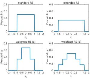
First, FK generalizes the sampling distribution in the natural number repre-sentation. The random sampling of the original RSR (which is called the standard RS) chooses only 0 or 1 with the equal probability. An extended version of the random sampling (the extended RS) is proposed in [4, 15], which extended the possible natural numbersdi∈ {0,1}todi ∈ {0,1, . . . , Ti}with equal probability.
Here, Ti is a small natural number such asTi= 3. FK generalizes the extended
random sampling furthermore so that a possible numberpfor the indexioccurs by a probability αip, where αip ≥ 0 and P
Ti
p=0αip = 1. In other words, the
sampling distribution is determined by ann×T matrixα = (αip) whereT is
the maximum ofTi over i. It is called the weighted RS. As ¯ζi is assumed to be
a uniformly distributed random variable, the probability ofζi is given as
Pζ(ζi) =
(
αip −p+12 ≤ ζ2i <−p2 or p2 ≤ ζ2i <p+12 (p≤T),
0 otherwise. (6)
Fig. 1 shows the examples of the probability distributions ofζifor the standard
RS, the extended RS, and the weighted RS. Note that the standard RS and the extended RS can sample all the possible natural number representations deter-ministically. Such deterministic sampling methods are mainly used in practice. On the other hand, the weighted RS cannot be actualized deterministically. Al-though the original FK employs a deterministic sampling method by allowing the dependence amongζi’s, it is assumed in this paper that everyζi is
indepen-dent of each other in order to facilitate the efficient calculation. It is because this paper focuses on the efficient estimation of the success probability more heavily than the construction of the deterministic sampling. Moreover, we discuss the relationship between our sampling distribution without the dependence and the previous deterministic methods in Section 6.2.
Second, FK improves the basis periodically so that the following target func-tionΦ(B) is reduced:
Φ(B) =
n
X
i=1
Fig. 1.Examples of probability distributions ofζi for the standard RS (T = 1,αip=
1
2), the extended RS (T = 2,αip= 1
3), the weighted RS (a) (T = 1,αi0= 2 3,αi1=
1 3),
Though it was partially explained by the normal approximation in [10] why this target function is effective, the explanation was insufficient (see Section 2.2).
2.2 Estimation of the Success Probability of Finding Very Short Lattice Vectors
In order to investigate the behaviors of RSR and its variants, it is important to estimate accurately the success probability that the current basis generates very short lattice vectors over a given random sampling. Here, we explain the two previous approaches for estimating the probability: the non-parametric ap-proach using the geometric description and the parametric one using the normal approximation.
Non-parametric Approach. The geometric description inspired by the Gaus-sian heuristic estimates the success probability by approximately counting the number of very short generated lattice vectors. The number can be defined as the intersection between all the generated lattice vectors and a ball with a very short diameterR. For example,Ris given as (1 +)`GHat the final stage of the SVP, whereis a small constant. The geometric description is a non-parametric estimation of the probability distribution, which gives a direct and accurate es-timation under an arbitrary sampling distribution. However, it was generally intractable to count the actual intersection because quite many lattice vectors are generated from a given basis. Recently, some state of the art methods were proposed for estimating the intersection in practice by dividing the lattice space into small partitions such as cylinders [11] and boxes [3] and utilizing various techniques for acceleration. Nevertheless, they are still time-consuming because their complexity depends on a large number of generated lattice vectors and small partitions. Moreover, it is difficult to investigate their estimation analyti-cally because it is non-parametric.
Parametric Approach. The normal approximation is a parametric approach under the randomness assumption and the central limit theorem [10]. It approxi-mates the probability distribution of the squared length`2of a generated lattice vector as a normal distribution whose parameters are only the mean and the variance. The mean of`2for a generated lattice vector is given as the first order moment of`2:
E `2=
n
X
i=1
E ζi2
kb∗ik2, (8) whereE() is the expectation operator over all the possible bases.ζiis the sum of
¯
ζi(a uniformly distributed random variable in [−12,12)) and ±2di (a half integer).
Fukase and Kashiwabara calculated E `2
analytically by assuming that every
di is equal to 0 [10]. The distribution of ¯ζi is formally given by
Pζ¯(x) = (
1 −1 2 ≤x <
1 2,
Then, the meanµ=E `2
is given as
µ=
n
X
i=1 kb∗ik
2Z
1 2
−1 2
x2dx= Pn
i=1kb ∗
ik
2
12 . (10)
Similarly, the second order momentE `4
is given as
E `4=
n
X
i=1
E ζi4
kb∗ik4+
n
X
i=1
E ζi2 kb∗ik2
n
X
j=1,j6=i
E ζj2 b∗j 2
, (11)
where we utilize the statistical independence between ζi and ζj (i 6= j) under
the randomness assumption. Then, the varianceσ2=E `4
−µ2 is given as
σ2=
n
X
i=1
E ζi4
kb∗ik4− Pn
i=1kb∗ik
4
144 =
Pn
i=1kb∗ik
4
180 . (12)
µandσ2 determine the simple normal distribution function which can be inves-tigated both numerically and analytically [10]. However, the serious weakness of this approximation is that the estimation is different from the actual distri-bution especially when the length of a generated lattice vector is very short as is pointed out in [3]. In other words, the normal approximation is too rough to estimate accurately the success probability. In addition, it does not consider any sampling distribution because every di is assumed to be a constant (0 in FK).
2.3 Gram-Charlier A Series
The normal approximation cannot estimate the actual distribution sufficiently accurately. In this paper, we improve the simple normal approximation by uti-lizing higher order cumulants. We employ the Gram-Charlier A series [7, 21] for this purpose. Here, we explain this technique in brief.
Overview. LetP(x) be a probabilistic distribution function satisfyingP(x)≥ 0 and R∞
−∞P(x) dx= 1. There are three well-known series expansion ofP(x): the Edgeworth series, the Gram-Charlier A series, and the Gram-Charlier B se-ries [7]. The Edgeworth sese-ries expansion is not suitable to estimate the success probability because it assumes that xis the sum of the independent and iden-tically distributed random variables. The Gram-Charlier B series expansion is also not suitable because the principal probability distribution is the exponen-tial one. Therefore, we employ the Gram-Charlier A series. We assume that the random variablexis normalized. In other words, its meanµand its varianceσ2
are 0 and 1, respectively. This assumption does not lose the generality because the variable ofP(x) is easily transformed by
P(z) = P(x)
σz
where x= (z−µz)/σz (µz andσz are the mean and the standard deviation of
z, respectively). Then, the Gram-Charlier A series ofP(x) is given as
P(x) = 1 + ∞ X
r=3
crHr(x)
!
e−x2 2
√
2π, (14)
whereHr(x) is ther-th degree Hermite polynomial defined as
Hr(x)e−
x2
2 = (−1)r d
r
dxre
−x2
2 . (15)
cr is ther-th coefficient depending on the r-th and lower order cumulants (the
details are described below). The series is guaranteed to converge if P(x)
de-creases faster thane−x 2
4 [6, 21]. This condition is generally satisfied in the search
in the natural number representation because there exists a boundT.
Cumulants. Here, we explain the cumulants, which are the most important statistics for the Gram-Charlier approximation. The cumulants ofP(x) are for-mally defined as follows. The cumulant generating functionK(t) is defined as
K(t) = log Z ∞
−∞
etxP(x) dx. (16)
The power series expansion ofK(t) is given as
K(t) = ∞ X
r=1
κr
tr
r!, (17)
where κr is the r-th order cumulant of P(x). By using the r-th derivative of
K(t),κr is given as
κr=K(r)(0). (18)
κris calculated in practice by the moments ofP(x). Ther-th order moment of
P(x) (denoted byµr) is given as
µr=
Z ∞
−∞
xrP(x) dx. (19)
Then, ther-th order cumulant is recursively given as
κr=µr− r−1 X
m=1 r−1
m−1
κmµr−m. (20)
following. Let κr(x) be ther-th order cumulant of a random variablex. Then,
the following equation holds:
κr(ax) =arκr(x), (21)
where a is an arbitrary constant. This property is called the homogeneity. If
xand y are statistically independent random variables, the following equation holds:
κr(x+y) =κr(x) +κr(y). (22)
This property is called the additivity. By utilizing these two properties under the randomness assumption, the distribution of the length of a generated lat-tice vector in the SVP is easily estimated. In addition, the following important property holds for any normal distribution: κr = 0 for r ≥ 3. Therefore, the
cumulant generating function of a normal distribution is given as
Knormal(t) =κ1t+
κ2t2
2 . (23)
When a random variablezis normalized tox= (z−κ1(z))/ p
κ2(z), the (nor-malized) cumulants ofx(denoted byλr) are given as
λr(x) =
κr(z)
(κ2(z))
r 2
(24)
forr≥3 (λ1= 0 andλ2= 1).
Coefficients. Here, we briefly explain the derivation of the Gram-Charlier A se-ries and give its coefficientcr. LetP(x) be any probability distribution function
of a normalized random variable x(see [21] for the details). The characteristic function ofP(x) (denoted byf(t)) is defined as
f(t) = Z ∞
−∞
eitxP(x) dx, (25)
where i is the imaginary unit. Using the cumulant generating function K(t),
f(t) is given as
f(t) =eK(it)= exp it+−t 2
2 +
∞ X
r=3
λr
(it)r
r! !
. (26)
On the other hand, the characteristic function of the unit normal distribution
(21πe−x 2
2 ) is given as
g(t) = exp
it+−t 2 2
Then,f(t) is given as
f(t) = exp ∞ X
r=3
λr
(it)r
r! !
g(t) = ∞ X p=0 1 p! ∞ X r=3 λr
(it)r
r! !p!
g(t)
= 1 + ∞ X
r=3
cr(it)r
!
g(t), (28)
where the Maclaurin series of the exponential function is utilized and cr is a
coefficient. Because the characteristic functionf(t) (replacingtwith−t) can be regarded as the inverse Fourier transform of any P(x), the following equation holds:
(−it)rf(t) = Z ∞
−∞
drP(x)
dxr e
itxdx. (29)
By applying the Fourier transformation tof(t), the following equation is derived:
P(x) = 1 + ∞ X
r=3
cr(−1)r
dr
dxr
!
e−x 2 2
2π = 1 +
∞ X
r=3
crHr(x)
!
e−x22
√
2π. (30)
This is the Gram-Charlier A series. Eachcqis the coefficient ofuqof the following
polynomialψ(u):
ψ(u) = ∞ X p=0 1 p! ∞ X r=3 λr ur r! !p . (31)
Thoughψ(u) includes the infinite summation,cq can be calculated from a finite
sets of the terms with r ≤ q and p ≤ q3. The complexity of calculating cq is
O qq3if everyλr(r≤q) is given.
There is another formulation of the coefficients, which is often more efficient than this usual formulation. See Section 6.4 for the details.
Cumulative Distribution Function. The cumulative distribution function ofP(x) is defined as
F(x) = Z x
−∞
P(x) dx. (32)
The integration of the Hr(x)e−
x2
2 is given as
Z x
−∞
Hr(u)e−
u2
2 du=−
Z x
−∞
dHr−1(u)e−
u2 2
du du=−Hr−1(x)e
−x2
2 . (33)
Therefore, the Gram-Charlier A series ofF(x) is given as
F(x) = Z x
∞
e−u22
√
2πdu−
∞ X
r=3
crHr−1(x) !
e−x22
√
2π, (34)
Examples. Lastly, we show the concrete examples of the Hermite polynomials
Hr(x) forr= 2, . . . ,9 and the coefficientscrforr= 3, . . . ,10 in the following:
H2(x) =x2−1,
H3(x) =x3−3x,
H4(x) =x4−6x2+ 3,
H5(x) =x5−10x3+ 15x,
H6(x) =x6−15x4+ 45x2−15,
H7(x) =x7−21x5+ 105x3−105x,
H8(x) =x8−28x6+ 210x4−420x2+ 105,
H9(x) =x9−36x7+ 378x5−1260x3+ 945x,
(35)
and
c3=
λ3 3!,
c4=
λ4 4!,
c5=
λ5 5!,
c6=
λ6+ 10λ23
6! ,
c7=
λ7+ 35λ3λ4
7! ,
c8=
λ8+ 56λ3λ5+ 35λ24
8! ,
c9=
λ9+ 84λ3λ6+ 126λ4λ5+ 280λ33
9! ,
c10=
λ10+ 120λ3λ7+ 210λ4λ6+ 126λ25+ 2100λ23λ4
10! .
(36)
3
Method
Here, we propose a method for estimating the success probability of succeeding in generating very short lattice vectors. This method is much more efficient than the other estimation methods because it uses a few parameters depending on the sampling distribution (α) and the norm of each column of the orthogonalized lattice basis (kb∗ik). The key idea of the proposed method is to approximate the probability distribution of the squared length `2 =P
iζ
2
i kb∗ik
2
assuming the randomness assumption. For this purpose, we need to calculate ther-th order moment of ζi2. As the probability of ζi is generally given by Eq.
(6) under the randomness assumption, the r-th order moment µr ζi2
is given as
µr ζi2
= T X p=0 2
Z p+12
p 2
αipζi2rdζi= T
X
p=0
αipβpr, (37)
whereβpr can be analytically calculated as
βpr=
(p+ 1)2r+1−p2r+1
(2r+ 1) 22r . (38)
Then, ther-th order cumulantκr ζi2
can be calculated by the following recur-sion:
κr=µr− r−1 X
m=1 r−1
m−1
κmµr−m. (39)
Note thatζ2
i andζj2are independent fori6=junder the randomness assumption.
Therefore, ther-th order cumulant of`2 is given as
κr `2= n
X
i=1
κr ζi2
kb∗ik2r, (40)
where we utilize the homogeneity and the additivity of the cumulants. Ther-th order normalized cumulant of`2is given byλ
r `2= √κr κr
2
. Then, the coefficients
of the Gram-Charlier A series (cr) are calculated byλ3, . . . , λr. LetQ≥3 be a
positive integer determining the degree of approximation. When`2is normalized to a random variable x, the Gram-Charlier approximation of the cumulative distribution functionF(x) is given as
¯
FQ(x) =
Z x
∞
e−u2 2
√
2πdu−
Q
X
r=3
crHr−1(x) !
e−x2 2
√
2π. (41)
As the shape of a cumulative distribution function is invariant under an affine transformation of the variable, the Gram-Charlier approximation of F(z) for
z=`2 is given as
FQ(z) = ¯FQ
z−κ 1 √
κ2
. (42)
FQ(z) is uniquely determined by the sampling distribution α = (αip), the
or-thogonalized lattice basis B∗ = b∗ij, and the degree of approximation Q.
Fi-nally,FQ
ˆ
`2gives the approximation of the success probability of generating a lattice vector whose squared length is shorter than a threshold ˆ`2. Note that ˆ`2
can be changed easily becauseFQ(z) can be calculated for anyz. For example,
is given asFQ
(1.05)2`2 GH
. The probability distributionPQ(z) = dFQ(z)/dz
is also easily calculated by Eq. (14) if necessary. The algorithmic description of the above process is given in Algorithm 2.
Algorithm 2The Gram-Charlier approximation of the cumulative distribution of the squared lengths of generated lattice vectors.
Require: α,B∗, andQ. Calculate the momentsµr ζ2
i
byα(r≤Q, the same hereinafter). Calculate the cumulantsκr ζi2
byµr ζi2
. Calculate the cumulantsκr `2
and the normalized onesλr `2
byκr ζ2 i
andB∗. Calculate the coefficientscr byλr `2.
return the approximate cumulative distributionFQ(z) (and the probability distri-butionPQ(z) if necessary).
The complexity of this algorithm isO n2+O(nQT) +O nQ2+OQQ3
(the calculations of every kb∗ik2, every µr ζi2
, every κr ζi2
, and every cr).
If T is a finite number, FQ(z) converges to the true probability for Q → ∞
[6, 21]. Unfortunately, no theoretical bound of Q has been achieved. However, the numerical experiments in Section 4 will show that FQ(z) can approximate
the actual distributions if Q is larger than 50. It will be also shown that the calculation time can be within one minute even for Q= 70.
There is another (often more efficient) algorithm using a different calculation method of the coefficients. See Section 6.4 for the details.
4
Experiment
Here, it is numerically verified whether the Gram-Charlier approximationFQ(z)
can estimate the actual success probability for various lattice basesBand various sampling distributionsα. The following four lattice bases are used:
– B128 was originally generated in TU Darmstadt SVP challenge [16] (n= 128, seed = 0) and was roughly reduced by the BKZ algorithm of the fplll package [20] with block size 20. The target function of FK was not reduced (Φ(B) = 195.3 where the Gaussian heuristic is normalized to 1).
– B128reducedwas reduced largely from B128 by a variant algorithm of FK (Φ(B) = 102.5).
– B100 was generated in the same way as B128 except forn= 100. – B150 was generated in the same way as B128 except forn= 150.
The following two sampling distributions are used, which are based on the stan-dard RS and the extended RS:
– 21735-RS consists of 217×35 ' 225 samples, where T
i was set to 3 for
n−5 ≤i≤n−1 and 2 forn−22≤i≤n−6 (Ti = 1 for the others). In
other words,di fori=n−5, . . . , n−1 is selected uniformly randomly from
0,1,2 instead of 0,1.
Note that the above sampling distributions were estimated accurately (namely, without any sampling error) because they enumerated all the possible samples deterministically. The weighted RS was not employed in this experiment because of its inevitable sampling error. The actual probability of the squared length`2 over a sampling on a basis was estimated by a histogram of the squared lengths over all the generated lattice vectors. The logarithm with base 2 of the cumulative distribution was used for displaying the result because it clarifies the differences among the cumulative distribution functions when`2 is short.
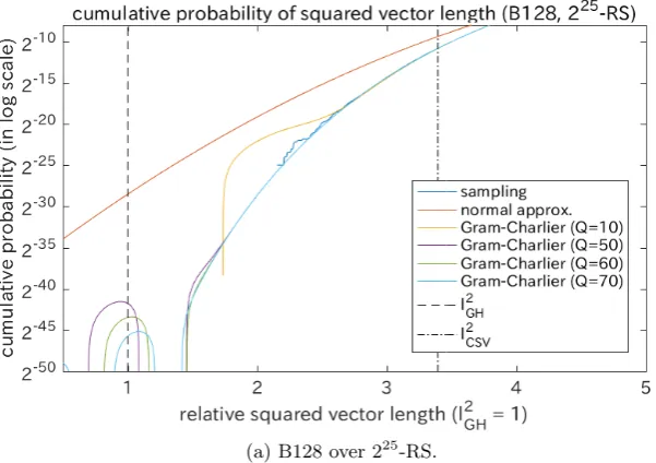
Fig. 2 shows the results for B128 and B128reduced over 225-RS. The actual distributions over the sampling are displayed by the bumpy blue curves. The normal approximation is displayed by the uppermost orange curve. The corre-sponding Gram-Charlier approximationsFQ(z) are also displayed (Q= 10, 50,
60, and 70). Note that the complete form of the approximation withQ= 10 can be described in Section 2.3. The approximation with the highest degree (Q= 70) is displayed by the light blue curve. The pre-estimated minimal squared length
`2
GH (by the Gaussian heuristic) is displayed by the dashed vertical line. The squared lengths of the generated lattice vectors are normalized so that `2
GH is equal to 1. Moreover, the squared length of the current shortest vector (namely, the first index) of the basis (denoted by `2
CSV) is displayed by the dot-dashed vertical line. First, we can observe thatFQ(z) estimated the actual distributions
quite accurately ifQis larger than 50. It verifies that our method is useful at least when the cumulative probability is more than 2−25. Next, we can observe that
FQ(z) withQ≥50 approximately converged to a decreasing curve at least when
the cumulative distribution is more than 2−50. Though it is hard to guarantee that these converged curves can estimate the actual cumulative probability, it can be asserted that the curves are accurate under the randomness assumption because they are determined only byαandB∗. Third,FQ(z) withQ≥50
con-verged around`2
CSV. Therefore, it can be determined easily whether the current shortest vector is improved by a given sampling distribution or not. Fourth, the converged curves fell sharply below thresholds around the Gaussian heuristic in comparison with the gently-reducing normal approximations. It shows that the curve for B128 cannot achieve a very short lattice vector even if the number of samplings is near the infinity. On the other hand, the curve for B128reduced seems to achieve the Gaussian heuristic by a sufficiently large number of sam-plings. The results show that it is crucial for finding a very short lattice vector to reduce the lattice basis.
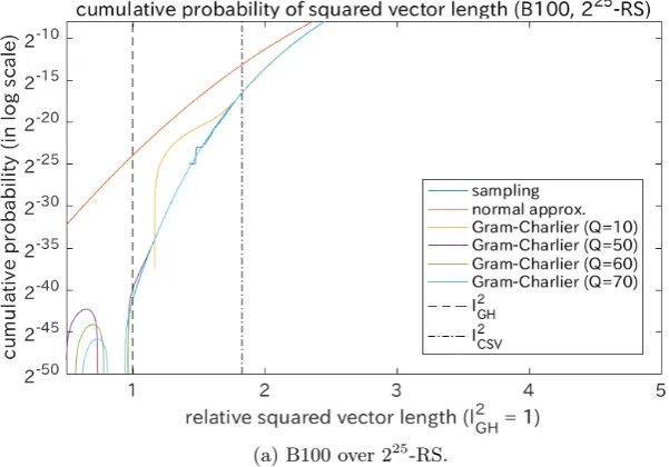
In order to verify the applicability of the Gram-Charlier approximations in various cases, different sizes of lattice bases (Fig. 3) and a different sampling dis-tribution (Fig. 4) were employed. Fig. 3 shows the results for different sizes of lat-tice bases (B100 and B150) over 225-RS. In both cases,FQ(z) withQ≥50
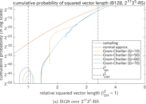
distribution. Fig. 4 shows the results of the bases with B128 and B128reduced over a different sampling distributions 21735-RS. The results were quite similar to those in Fig. 2, whereFQ(z) withQ≥50 converged to a curve and could
es-timate the actual cumulative distribution accurately. In summary, these results verify that the Gram-Charlier approximations are useful for various lattice bases and various sampling distributions.
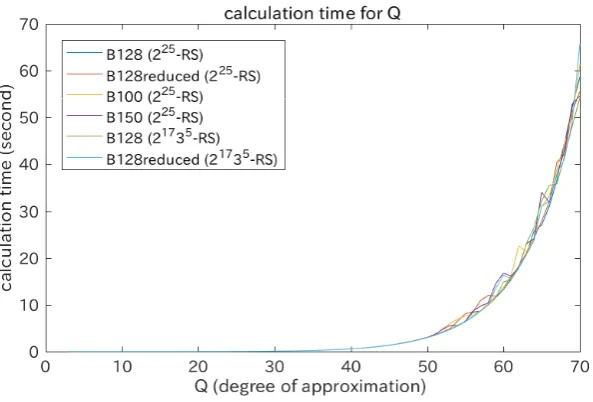
Regarding the efficiency of our method, Fig. 5 shows the actual calculation time for the above experimental settings ({B128, B128reduced, B100, B150} over 225-RS and {B128, B128reduced} over 21735-RS). for various degrees of approximationQfrom 3 to 70. It shows that the calculation time mostly did not depend on the lattice bases nor the sampling distribution. However, the time is increased exponentially according to the degree of approximation Q. The time was within about one minute even for the largestQ= 70. The state of the art method proposed by Aono and Nguyen could estimate the success probability for one natural number representation within about 2 seconds (see Table 1 in Section 5.4 of [3]). Note also that their method estimates essentially only one point in the cumulative distribution curve because it is non-parametric. Though [3] proposed some acceleration techniques such as random sampling and parallel computing, it does not seem to be available for exponentially increasing number of samples. On the other hand, our parametric method can estimate the complete form of the curve over 250 natural number representations. It shows that our method is much more efficient than the state of the art method [3]. In addition, our method could give sufficiently accurate results at least within the observable range.
In summary, the numerical experiments verified the following points. First, if the cumulative probability is larger than 2−25, the Gram-Charlier approxima-tionFQ(z) with Q≥50 can estimate accurately the actual distribution of the
squared length of generated lattice vectors for any lattice bases and any sampling distributions. Second, FQ(z) with Q ≥ 50 converges to a curve at least when
the cumulative probability is larger than 2−50. Because the computation over 250-RS is expected to take hundreds of years [19], the limit 2−50 is sufficiently small in practice. Third,FQ(z) can be calculated efficiently within one minute
even for the largestQ= 70.
5
Investigation of RSR and FK
Here, we investigate RSR and its variant FK by the Gram-Charlier approxima-tion in order to clarify why FK is superior to other methods in the SVP. Note that the following investigation is actualized only by the proposed Gram-Charlier approximation. It is quite hard for the non-parametric approach to investigate the detailed behavior of the algorithms over a huge size of samples such as 250.
5.1 Utilization of Weighted Sampling Distribution
(a) B128 over 225-RS.
(b) B128reduced over 225-RS.
Fig. 2.Cumulative distributions of the squared length from the bases with n = 128 over 225-RS and the Gram-Charlier approximations: The histograms of the squared lengths of the 225 generated lattice vectors are displayed by blue (slightly bumpy)
curves. The curves of the normal approximation (in orange) and the Gram-Charlier approximations FQ(z) (Q = 10, 50, 60, and 70) are also displayed. The Gaussian heuristic`2GH (normalized to 1) is displayed by the dashed vertical line. The squared
length of the current shortest vector`2CSV is displayed by the dot-dashed vertical line.
(a) B100 over 225-RS.
(b) B150 over 225-RS.
(a) B128 over 21735-RS.
(b) B128reduced over 21735-RS.
Fig. 5.Calculation time for various degrees of approximation: The actual calculation time for the Gram-Charlier approximation was measured for {B128, B128reduced, B100, B150}over 225-RS and{B128, B128reduced}over 21735-RS. The degree of ap-proximationQwas set from 3 to 70.
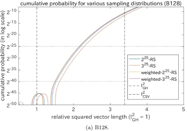
We used the two lattice bases B128 and B128reduced in Section 4. 225-RS and 325-RS were employed as an example of the standard RS and that of the ex-tended RS, respectively. They consist of 225 and 325 ' 240 possible samples. The natural number for each index occurs equally in 0,1 for 225-RS or 0,1,2 for 325-RS. FK can give different weights to each natural number p. It is suggested in [10] that the inverse of βp1 of Eq. (38) gives an appropriate weight, where
β11 = 121, β21 = 127, and β31 = 1912. Therefore, the appropriate weighted distri-bution is given as (αi1, αi2) ∝ 1,17
forTi = 2 and (αi1, αi2, αi3)∝ 1,17, 1 19
for Ti = 3. Two sampling distributions were constructed by applying the
ap-propriate weighted distribution to 225-RS and 325-RS, which are referred as to weighted-225-RS and weighted-325-RS. Each of the two sampling distributions corresponds to an example of the weighted RS.
resources are available. On the other hand, the maximum number of samples over weighted-325-RS is about 240. Therefore, the cumulative probability can be reduced to the lower horizontal line if available. It is expected to generate shorter lattice vectors than weighted-225-RS.
5.2 Periodical Improvement of Current Basis by Target Function
Another important feature of FK is that it periodically improves the basis so that the target function Φ(B) of Eq. (7) is reduced. Fukase and Kashiwabara [10] attempted to explain why this feature can accelerate the SVP by the normal approximation, whereΦ(B) can be regarded as the mean of `2 over generated lattice vectors. They asserted that the success probability becomes higher as the mean of`2is smaller. Though this tendency is also observed in the form of the Gram-Charlier approximation ofFQ(z), it is not essential to utilize higher order
cumulants. However, it cannot be explained by the normal approximation why the basis needs to be improved periodically. Although the normal approximation in Fig. 2 seems to achieve `2GH by using about 230 samples even for the initial basis B128, it is not true. Here, the investigation with the Gram-Charlier ap-proximation is carried out for explaining why the periodical improvement of the basis is essential.
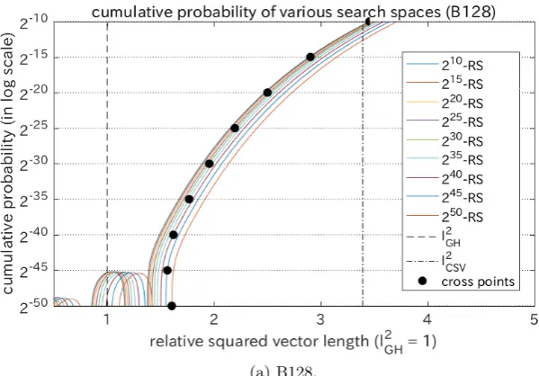
Fig. 7 shows the Gram-Charlier approximations over the 2u-RS, which is
denoted by F70(z; 2u). The exponent parameter u determines the size of the search space over the random sampling distribution.uwas set to 10, 15, 20, 25, 30, 35, 40, 45, and 50. B128 and B128reduced are employed as the basis. The horizontal lines correspond to the lower bounds of the cumulative probability 2−u. Each black circle displays a cross-point between F
70(z; 2u) and the cor-responding lower bound 2−u. Asubecomes larger, the cumulative distribution
gets worse because the distribution moves to the right. On the other hand, asu
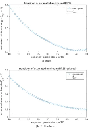
becomes larger, the lower bound of the cumulative distribution becomes smaller (namely, better) because the search space becomes larger. Each cross-point rep-resents an equilibrium point between the above two factors. We can regard the squared length at the cross-point as an estimated minimum for given u. The estimated minimum is calculated by solving the following equation with respect toz for givenu:
F70(z; 2u) = 1
2u. (43)
It is easily solved numerically because it is a continuous single-variable function. Fig. 8 shows the transitions of the estimated minimum of the squared length of generated lattice vectors for u = 10, . . . ,50. It shows that the estimated minimum for B128 is saturated to about 1.5 even if 2u is intractably large. In
(a) B128.
(b) B128reduced.
Fig. 6. Cumulative distributions of the squared length from B128 and B128reduced over the weighted RS: The Gram-Charlier approximationsF70(z) are displayed over the
Though it may be because the estimated minimum is based on the probabilistic search which allows duplicate samples, it is beyond the scope of this paper to clarify this phenomenon.
6
Discussions
6.1 Validity of Randomness Assumption
The accuracy of our method heavily relies on the randomness assumption. Re-versely, the converged Gram-Charlier approximation with sufficiently large Q
is rigorously accurate if the randomness assumption holds. Though it is hard currently to verify the validity of the randomness assumption, the assumptions on the Gaussian heuristic [12] suggest that its validity depends on the relative squared vector length `2/`2
GH. If the relative length is 1 (namely, `
2 is equal to`GH), the randomness assumption does not hold because the distribution in-cludes only one sample. On the other hand, if the relative length is sufficiently large, the randomness assumption seems to be valid because the number of pos-sible lattice vectors within the corresponding volume is expected to be high. Letting`2/`2
GHbe 1 +, the number is approximately estimated as (1 +)
n 2. For
example, it is 1.164'445 forn= 128 and= 0.1. The estimated number seems to be sufficiently high to approximate a continuous distribution even for such a small= 0.1.
6.2 Dependence among Indices of Natural Number Representation
One of the disadvantages of our proposed model is that it cannot allow the de-pendence among the indices of the natural number representation (see Section 2.1). In addition, our model seems to be based on an inefficient non-deterministic search. On the other hand, almost all of the state of the art algorithms employ a deterministic search enumerating a set of candidate natural number representa-tions, where the dependence among the indices is often allowed. Here, we show that our model can give a probabilistic approximation of such a deterministic search and the optimalαcan be calculated by minimizing the Kullback-Leibler divergence. In other words, by regarding any set of candidate natural number representations in any algorithm as a probability distribution, our model can ap-proximate this distribution as accurately as possible. Though there are various metrics such as the Euclidean distance, we employed the Kullback-Leibler diver-gence here. It is because its optimum can be derived easily and its mathematical properties have been extensively investigated [5].
When only a single natural number representation d = (di) is given, we
can estimate the Gram-Charlier approximation of the conditional probability
PQ(z|d) by letting αip be 1 only if p = di (otherwise αip = 0). Let Ω be
(a) B128.
(b) B128reduced.
Fig. 7. Cumulative distributions of the squared length from B128 and B128reduced over the various search spaces 2uof RS: The Gram-Charlier approximationsF70(z; 2u)
(a) B128.
(b) B128reduced.
Fig. 8. Estimated minimum of the squared length from B128 and B128reduced for the exponent parameter u of RS: The parameter u of 2u-RS determines the size of
the search space. Each estimated minimum corresponds to a cross-point in Fig. 7. The squared length of the current shortest vector`2CSVis displayed by the dot-dashed
PQ(z) is given as
PQ(z) =
X
d
PQ(z|d)P(d) =
P
d∈ΩPQ(z|d)
|Ω| , (44)
where|Ω|is the cardinality (the number of members) ofΩ. P(d) is the proba-bility that doccurs in the search, which is defined as
P(d) = ( 1
|Ω| d∈Ω,
0 otherwise. (45)
We can estimate PQ(z) over any Ω by these equations. However, the
calcula-tion is time-consuming because it requires the estimacalcula-tion of PQ(z|d) for every
d∈Ω. Our proposed model is essentially equivalent to employing the following approximation:
P(d)'Y
i
P(di) =
Y
i
αidi. (46)
PQ(z) is efficiently calculated by our model, because the summation over Ω
can be divided into the estimation of an independent probability distribution for each indexi (see Section 3). Now, the Kullback-Leibler divergence between
P(d) andQ
iαidi is given as
DKL P(d)| Y
i
αidi
!
=X
d
P(d) log
P(d)
Q
iαidi
=X
d∈Ω
1 |Ω|log
1
|Ω|Q
iαidi
=−log (|Ω|)− P
d∈Ω
P
ilog (αidi)
|Ω| . (47)
This divergence is equal to 0 only if the two distributions are completely the same, and otherwise always positive. Therefore, Q
iαidi can approximateP(d)
as accurately as possible by minimizingDKL. Then, the optimum ofα(denoted ˆ
α= ( ˆαip)) is given as
ˆ
α= arg max α
X
d∈Ω
X
i
log (αidi) subject to
X
p
αip= 1. (48)
By the method of Lagrange multipliers, ˆαip is given as
ˆ
αip=
P
d∈Ωδpdi
|Ω| , (49)
where δpdi is the Kronecker delta. In other words, ˆαip is proportional to the
number of occurrences ofpin the indexiofΩ. It is easily calculated for anyΩ. Reversely, there is also a promising approach from our proposed model to a deterministic search framework. For a given natural number representation
d = (di), its occurrence probability is given as Qiαidi. Then,
Q
regarded as a score measuring the “goodness” of d. Using the logarithm, the scoreϕ(d) is given as
ϕ(d) =X
i
logαidi. (50)
ϕ is the sum of weights, each of which depends on only the index i and di. If
the natural number representations with high scores can be collected, we can construct deterministically a setΩincluding only the “better” candidates. This principle is similar to the enumeration of the lattice vectors with the smaller lengths in the previous lattice basis reduction algorithms. Therefore, our pro-posed model is promising for improving the previous algorithms.
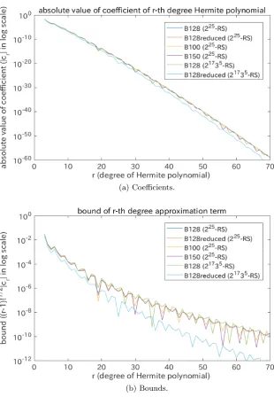
6.3 Convergence Property of Gram-Charlier Approximation
Here, we investigate experimentally the convergence property of the Gram-Charlier approximation of the cumulative distribution function with the degree of approximation. One of the important factors is the convergence of cr (the
coefficients of the Hermite polynomialsHr(x)). Another important factor is the
convergence of the value ofcrHr−1(x). The bound of|Hr(x)|is given as
|Hr(x)|<1.09π
1 4e
x2 4
√
r!, (51)
which holds for anyrandx(see 22.14.17 and 22.5.19 in [1].) Therefore,crHr−1(x) converges if p(r−1)!cr converges. Fig. 9 shows the transitions of |cr| and
|p
(r−1)!cr| for 3 ≤ r ≤ 70. Note that cr is determined only by the basis
and the sampling distribution. We used{B128, B128reduced, B100, B150}over 225-RS and{B128, B128reduced} over 21735-RS. Fig. 9 experimentally verified that the coefficients and the bounds converges to 0 roughly exponentially. It is interesting that the transitions are similar irrespective of the basis and the sampling distribution. It suggests that some theoretical approximations may be available.
6.4 Accelerated Algorithm for Estimating Coefficients
The standard formulation of the coefficients of the Gram-Charlier approximation is given in Section 2.3. Here, another formulation is utilized, which can accelerate Algorithm 2. The new formulation is based on the orthogonality property of the Hermite polynomials, which is given as
Z ∞
−∞
Hp(x)Hq(x)e−
x2 2 dx=
√
2πp!δpq. (52)
Using this property, the expectation ofHr(x) (r≥3) over a normalized
proba-bility distribution functionP(x) is given as
Z ∞
−∞
(a) Coefficients.
(b) Bounds.
Fig. 9.Transitions of the coefficients and the bounds of the Hermite polynomials:|cr|
and p
(r−1)!|cr|(3≤r ≤70) are calculated for {B128, B128reduced, B100, B150}
where cr is the r-th coefficient of the Gram-Charlier approximation. Now, the
explicit expression ofHr(x) is given as
Hr(x) =r!
br 2c
X
p=0
(−1)px(r−2p)
2pp! (r−2p)!. (54)
Then,cris given as
cr=
br 2c
X
p=0
(−1)pµr−2p(x)
2pp! (r−2p)! , (55)
where µr−2p(x) is the (r−2p)-th order moment of a random variable x over
P(x). In the similar way as in Eq. (39), µr(x) can be calculated recursively
from the normalized cumulantsλrby
µr=λr+ r−1 X
m=1 r−1
m−1
λmµr−m. (56)
Consequently, the new algorithm calculating the coefficients is given as follows.
Algorithm 3The accelerated Gram-Charlier approximation of the cumulative distribution of the squared lengths of generated lattice vectors.
Require: α,B∗, andQ. Calculate the momentsµr ζi2
byα(r≤Q, the same hereinafter). Calculate the cumulantsκr ζi2
byµr ζi2
.
Calculate the cumulantsκr `2and the normalized onesλr `2byκr ζi2
andB∗. Calculate the momentsµr `¯2
byλr `2. Calculate the coefficientscr byµr `¯2
.
return the approximate cumulative distributionFQ(z) (and the probability distri-butionPQ(z) if necessary).
Here, ¯`2 denotes the normalized squared length. This algorithm avoids the combinatorial problem in the direct estimation of the coefficients from the mulants by utilizing an additional step calculating the moments from the cu-mulants. Because the bottleneck process is the recursive interconversion be-tween the moments and the cumulants, the complexity of this algorithm is
O n2
+O(nQT) +O nQ2
, where the term ofOQQ3
is removed. Therefore,
7
Conclusion
In this paper, we proposed a new method for estimating the success probability of finding very short lattice vectors in the lattice basis reduction algorithm. The proposed method is based on a parametric approach using the Gram-Charlier approximation and gives a closed-form expression with a few parameters. It could estimate the actual distribution quite accurately and quite efficiently. The in-vestigations with the proposed method discovered some important properties of RSR and FK. The most significant advantage of the proposed method is that it can estimate the success probability quite efficiently with keeping the accuracy. The investigation in Section 5 is intractable for the non-parametric approach because it needs to manage 250-RS. On the other hand, the Gram-Charlier ap-proximation estimated all the distributions within at most one minute. The ex-perimental results showed that the calculation time and the accuracy of our pro-posed method do not depend on the lattice basis and the sampling distribution. In other words, they verified that our method is useful for a high-dimensional lattice over a large number of samplings.
An unsolved problem of the proposed method is that we have not clarified yet the theoretical relationship between the degree of approximationQand the convergence of the estimation. We are planning to investigate the relationship furthermore in order to setQto an appropriate value. In addition, we are plan-ning to investigate furthermore the validity of the randomness assumption by the Gram-Charlier approximation. Another problem is that the Gram-Charlier ap-proximation was used only for verifying the superiority of the previous algorithms in this paper. It is promising to use this method for finding the optimal settings and parameters adaptively and for solving the SVP much more efficiently. For example, we are planning to estimate the optimal weighted sampling distribu-tion according to a given basis and to set the optimal size of the search space by
u. Moreover, we are planning to investigate the state of the art algorithms (for example, [3], [19], and [8]) by the approximation method in Section 6.2.
References
1. Abramowitz, M., Stegun, I.A.: Handbook of mathematical functions with formulas, graphs, and mathematical table. Dover New York (1965)
2. Ajtai, M., Kumar, R., Sivakumar, D.: A sieve algorithm for the shortest lattice vector problem. In: Proceedings of the Thirty-third Annual ACM Symposium on Theory of Computing. pp. 601–610. STOC ’01, ACM, New York, NY, USA (2001),
http://doi.acm.org/10.1145/380752.380857
3. Aono, Y., Nguyen, P.Q.: Random sampling revisited: Lattice enumeration with discrete pruning. In: EUROCRYPT (2). pp. 65–102. Springer (2017)
5. Burnham, K.P., Anderson, D.R.: Model selection and multimodel inference: A practical-theoretic approach. Springer-Verlag, Berlin; New York, 2 edn. (2002) 6. Cram´er, H.: On some classes of series used in mathematical statistics. In:
Proceed-ings of the Sixth Scandinavian Congress of Mathematicians. pp. 399–425 (1925) 7. Cram´er, H.: Mathematical Methods of Statistics. Princeton mathematical series,
Princeton University Press (1946)
8. Ducas, L.: Shortest vector from lattice sieving: A few dimensions for free. In: Nielsen, J.B., Rijmen, V. (eds.) Advances in Cryptology – EUROCRYPT 2018. pp. 125–145. Springer International Publishing, Cham (2018)
9. Fincke, U., Pohst, M.: Improved methods for calculating vectors of short length in a lattice, including a complexity analysis. Mathematics of computation 44(170), 463–471 (1985)
10. Fukase, M., Kashiwabara, K.: An accelerated algorithm for solving SVP based on statistical analysis. JIP 23, 67–80 (2015)
11. Gama, N., Nguyen, P.Q., Regev, O.: Lattice enumeration using extreme pruning. In: Gilbert, H. (ed.) Advances in Cryptology – EUROCRYPT 2010: 29th An-nual International Conference on the Theory and Applications of Cryptographic Techniques, French Riviera, May 30 – June 3, 2010. Proceedings. pp. 257–278. Springer Berlin Heidelberg, Berlin, Heidelberg (2010),https://doi.org/10.1007/ 978-3-642-13190-5_13
12. Hoffstein, J., Pipher, J., Silverman, J.: An Introduction to Mathematical Cryptog-raphy. Springer Publishing Company, Incorporated, 2 edn. (2014)
13. Kannan, R.: Improved algorithms for integer programming and related lattice problems. In: Proceedings of the Fifteenth Annual ACM Symposium on The-ory of Computing. pp. 193–206. STOC ’83, ACM, New York, NY, USA (1983),
http://doi.acm.org/10.1145/800061.808749
14. Lenstra, A., Lenstra, H., Lov´asz, L.: Factoring polynomials with rational coeffi-cients. Mathematische Annalen 261(4), 515–534 (12 1982)
15. Ludwig, C.: Practical lattice basis sampling reduction. Ph.D. thesis, Technische Universit¨at Darmstadt (2006)
16. Schneider, M., Gama, N.: SVP challenge, available at https://www. latticechallenge.org/svp-challenge/
17. Schnorr, C.P., Euchner, M.: Lattice basis reduction: Improved practical algorithms and solving subset sum problems. Math. Program. 66(2), 181–199 (Sep 1994),
http://dx.doi.org/10.1007/BF01581144
18. Schnorr, C.: Lattice reduction by random sampling and birthday methods. In: Alt, H., Habib, M. (eds.) STACS 2003, 20th Annual Symposium on Theoretical Aspects of Computer Science, Berlin, Germany, February 27 - March 1, 2003, Proceedings. Lecture Notes in Computer Science, vol. 2607, pp. 145–156. Springer (2003) 19. Teruya, T., Kashiwabara, K., Hanaoka, G.: Fast lattice basis reduction suitable
for massive parallelization and its application to the shortest vector problem. In: Public-Key Cryptography - PKC 2018 - 21st IACR International Conference on Practice and Theory of Public-Key Cryptography, Rio de Janeiro, Brazil, March 25-29, 2018, Proceedings, Part I. pp. 437–460 (2018)
20. The FPLLL development team: fplll, a lattice reduction library (2016), available athttps://github.com/fplll/fplll