Volume 2009, Article ID 697451,10pages doi:10.1155/2009/697451
Research Article
False Alarm Rate Estimation for Information-Theoretic-Based
Source Enumeration Methods
Matthew T. Brenneman and Yu T. Morton
Department of Electrical & Computer Engineering, Miami University, Oxford, OH 45056, USA
Correspondence should be addressed to Matthew T. Brenneman,[email protected]
Received 6 March 2009; Revised 5 July 2009; Accepted 15 October 2009
Recommended by Husheng Li
The Tracy-Widom distribution is used to determine the false alarm rate of information theoretic methods that statistically estimate the number of sources in a multichannel receiver input. The Tracy-Widom distribution is the limiting distribution for the largest eigenvalue of a covariance matrix having a central white Wishart distribution. Such covariance matrices are produced by the output of multi-channel receivers whose signals can be characterized as zero-mean Gaussian processes. The Tracy-Widom distribution is used to estimate the false alarm rate of the Akaike Information Criterion and Minimum Description Length methods when no external sources are present. The Tracy-Widom distribution along with the eigenvalue inclusion principle is used to obtain an upper bound on the false alarm rate of the Akaike Information Criterion and Minimum Description Length when one external source is present. Monte-Carlo simulations were performed to demonstrate the effectiveness of both methods for cases where both the array and data sample sizes are small.
Copyright © 2009 M. T. Brenneman and Y. T. Morton. This is an open access article distributed under the Creative Commons Attribution License, which permits unrestricted use, distribution, and reproduction in any medium, provided the original work is properly cited.
1. Introduction
The performance of information-theoretic-based methods for model selection is difficult to analyze for small sample sizes. Such a performance analysis is necessary because these methods are based on asymptotic approximations which are invalid for small samples [1]. In signal processing applications, scenarios occur when small sample sizes may be necessary or desirable to use (e.g., smart antennas signal pro-cessing for moving platforms). In this paper, we introduce a new method to evaluate the small sample performance of two information-theoretic-based methods commonly used in signal processing for a specific type of model selection: estimating the number of directional sources from the output signal of an array.
In this paper, we will analyze the small sample per-formance of the Akaike Information Criterion (AIC) [2,
3] and the Minimum Description Length (MDL) [4, 5], two commonly used information-theoretic approaches for source enumeration [6]. Because the focus of this paper is the small sample performance of information-theoretic methods for source enumeration, rather than determining which method for source enumeration is best, we will not
consider other methods for source enumeration that exist [7,
8] in our analysis. Early analyses show that for large sample sizes, the MDL is a consistent estimator for the number of sources, while the AIC tends to overestimate the number of samples [9]. Subsequent performance analyses for arbitrary sample sizes, however, have either relied on the use of large array sizes [10], large sample sizes [10,11], computationally expensive Monte-Carlo simulations [12], or involved the use of quantities which are difficult to evaluate numerically [13]. In this paper, we introduce a method to estimate the false-alarm rate (FAR) for the AIC and MDL. The contribution of our approach is that it can be used for arbitrary array and data sizes and is simple and computationally inexpensive to use, thereby making it practical for use in real-time applications.
zero-mean Gaussian processes. It will be shown that the utility of the TW distribution derives from two important properties it possesses. First, the TW distribution transforms the largest eigenvalue into a standardized random variable whose distribution is independent of the array and sample size [15,16]. GivenKarray elements, from whichNsamples are collected, the largest eigenvalue of the sample covariance matrix, λ1, can be used to construct the standardized test
statistic z = (λ1 −μK,N)/σK,N. Although μK,N and σK,N
are functions of N and K, the TW distribution of the standardized random variable,z, is the same forallvalues of
K andN.Thus, regardless of the array size or the number of samples, the P-value of z can be determined from a single table for the values of the TW cumulative distribution function (CDF) just like the standard normal distribution. Second, the TW distribution is applicable over virtually any size of array and input sample size (despite the fact that the TW was originally derived as the distribution for λ1
in the limit of both K andN going to infinity) [16]. This marks an important distinction between the TW distribution and the distributions for the largest eigenvalue derived from previous studies. The exact distribution of the largest sample eigenvalue has been derived for arbitrary array sizes but is only valid in the limit of large sample sizes [17]. A later attempt to derive an approximation to the exact distribution valid for finite sample sizes required the use of expressions that are difficult and computationally expensive to evaluate numerically [18]. Although an exact distribution for the largest eigenvalue for any sample and array size exists, it too is difficult to numerically evaluate efficiently [19]. In the case of [18,19], the evaluation of their distributions requires computing the ratio of an incomplete Gamma function and a complete Gamma function, whose arguments are both on the order of the sample size. Attempts to obtain reliable approximations to these ratios are cumbersome, complicated, and require the use of look-up tables [18]. On the other hand, it will be demonstrated that the TW distribution is simple, straightforward to use, and agrees well with the right-hand tail of the distribution for the largest eigenvalue of the sample covariance matrix for array sizes fromK=3 toK =9 and with sample sizes that range from the minimum number of samples required to estimate the covariance matrix well (which is max(3∗K, 2∗K−3) [20]) up to 20∗K.
The outline of the paper will be as follows. InSection 2, we present the TW distribution and compare its distribu-tional behavior to that of the largest eigenvalue from sample covariance matrices for small array and data sample sizes.
In Section 3, the AIC and MDL will be derived under the
condition that the variance in the input noise is known. In
Section 4, the TW law is used to estimate the FAR for the AIC
and MDL when there is no external source and when there is only one external source present, respectively. InSection 5, we summarize the results of the paper.
2. The Tracy-Widom Law
The TW law states that a standardized form of the largest eigenvalue for a covariance matrix having a central
white Wishart distribution approaches a unique limiting distribution. Consider N random vectors with K compo-nents, Xn, with multivariate normal distribution Xn i.∼i.d.
Nβ(0,σ2IK) forn = 1,. . .,N, where σ2 denotes the noise
variance andIKis theKbyKidentity matrix. Following the
notation of Dyson [21],β = 1 andβ = 2 indicate the real and complex normal distributions, respectively. The sample covariance matrix,R, is constructed from the data samples (from which their mean has been subtracted) using R =
(1/N)(Nn=1XnXnH), where superscript H denotes conjugate
transpose.
The eigenvalues of R, called the sample eigenvalues, are determined and ranked according to their magnitude such thatλ1 ≥ · · · ≥ λK.Under these conditions, the TW law
states that:
zdef= λ1−μK,N
σK,N
D
−−−→Fβ as K
N −→c0< c <1, (1)
where
μK,N=
√
K+N−2 +β2
N ,
σK,N=
√
K+N−2 +β N
⎡ ⎣√1
K +
1
N−2 +β
⎤ ⎦
1/3
, (2)
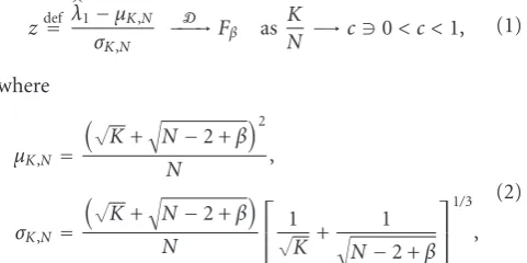
and Fβ is the TW CDF, shown in Figure 1. Fβ must be
computed numerically, and its values have been tabulated to four significant digits forzvalues in increments of 0.01 [22]. A complete published table for both F1 and F2 is
available [23] and a downloadable copy of these files is also available on the MatLab Central website (see http://
www.mathworks.com/matlabcentral/fileexchange/24590. In
this sense, the TW distribution works the same way as the standard normal distribution, which also must be numerically computed and requires a single look-up table for its use. Since only complex covariance matrices will be considered in our analysis,F2will be used exclusively from
this point on.
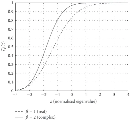
Figure 2plots the difference betweenF2and the empirical
cumulative distribution functions (ECDF) with respect toz
forK=2, 3, 5, 7, and 9. The ECDF for eachKwas generated from one million Monte-Carlo simulations, usingN = 3K
random samples on each trial. Based on this figure, we observe the following four important relationships between the TW distribution and the distribution for the largest sample noise eigenvalue.
Observation 1. The TW distribution provides a good approx-imation to the right-hand tails of the largest eigenvalue’s distribution function even whenKandNare small.
Figure 2shows that the agreement between the ECDFs
and the TW CDF is good in the right-hand tail of the distributions. Aroundz= −1.0 (which according toFigure 1
0 0.1 0.2 0.3 0.4 0.5 0.6 0.7 0.8 0.9 1
Fβ
(
z
)
−4 −3 −2 −1 0 1 2 3 4 z(normalised eigenvalue)
β=1 (real) β=2 (complex)
Figure1: The cumulative distribution functions of the TW
distri-butions for real and complex white Wishart covariance matrices as a function of the standardized random variablezgiven in (1).
−0.02 0 0.02 0.04 0.06 0.08 0.1 0.12 0.14 0.16 0.18
F2
(
z
)
−
ECDF
K
(
z
)
−3.5 −3 −2.5 −2 −1.5 −1 −0.5 0 0.5 1 z=(λ1−μK,N)/σK,N
ECDF2
ECDF3
ECDF5
ECDF7
ECDF9
Figure 2: The difference inF2, the TW CDF, and the empirical
CDFs ofzfor various values ofKusingN=3K.The two classes of distributions are in good agreement pastz= −1, the 80th percentile level forF2.
the TW distribution is less than 1% for all values ofK. A more quantitative look at the agreement between the right-hand tail of the TW distribution with that of the ECDFs is shown inTable 1. The CDF for the standardized form of the largest sample eigenvalue was estimated at threezvalues corresponding to the CDF values for the TW distribution at 90%, 95%, and 99%. The ECDF values were determined for 5 different array sizes (K = 2, 3, 5, 7, and 9) withN =3K.
The last column gives an estimate for twice the standard error (SE) of the ECDF values based on that obtained from
Table1: ECDF values for the 90%, 95%, and 99 %F2CDF Values.
F2CDF (in %) ECDF Values (%) forN/K=3 2∗SE (in %)
K=2 K=3 K=5 K=7 K=9
90 90.97 90.74 90.54 90.41 90.035 ±0.06
95 95.85 95.65 95.46 95.53 95.25 ±0.04
99 99.23 99.18 99.11 99.07 99.05 ±0.02
binomial sampling, SE = p(1−p)/NSIMS, where pis the
true CDF value, and the number of simulations NSIMS =
106. Despite the agreement between the values of the TW
CDF and the ECDFs, the difference between them typically exceeds 2 SE units, and is therefore statistically significant.
Observation 2. The distribution for the standardized largest sample noise eigenvalue is stochastically less than the TW distribution.
Figure 2shows that forz >−1, the sign of the difference
in the CDFs is always negative. An important consequence of this observation is thatP(z ≥Z |z =(λ1−μK,N)/σK,N)≤
P(z ≥ Zz ∼ F2) for allZ > −1. Thus, we see that
if the TW distribution is used to approximate the true distribution for the largest sample noise eigenvalue, it will always overestimate the probabilities of events in the right-hand tail of the distribution.
Observation 3. AsK increases, while K/N is held constant, the normalized largest sample noise eigenvalue’s distribution functions approach the TW distribution.
This observation is a direct consequence of (1).Figure 2
illustrates this fact since the ratio ofN/Kis fixed at 3 for all of the ECDF curves.Figure 2, along withTable 1, shows that not only does the convergence occur asKincreases, but that it is relatively rapid.
Observation 4. The agreement between the TW and stan-dardized largest noise eigenvalue’s distribution generally improves as theP-value decreases (forP-values<10%).
The agreement between the TW CDF and the ECDFs shows a general uniform improvement forz >−0.5, which is a fraction of a percentile past the 90% CDF value forF2.
The relationship between the TW distribution and the limiting distribution of the standardized sample eigenvalue in the limit as N goes to infinity (while K is held fixed) is difficult to determine. Technically, they are not required to converge, since the hypothesis required for the TW law to hold, that the ratio of K/N to converge to a positive number less than one, is not satisfied. It is known that as
90.2 90.3 90.4 90.5 90.6 90.7 90.8 90.9 91
ECDF
at
F2
90%
le
ve
l
(
%)
0 50 100 150 200
N(number data samples) K=3
K=5 K=9
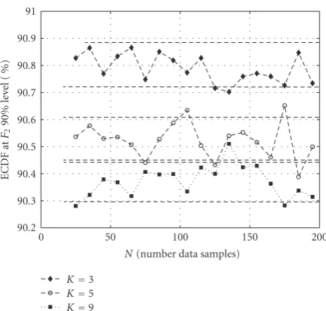
Figure3: The ECDF values at the 90% level forF2are computed as
a function of the number of data samples for three different array sizes. The dashed lines give a bounds of±1σabout the mean.
goes to zero as N → ∞, so does the scale factor σK,N.
Although this problem is not of central importance in our analysis (which focuses on small sample sizes), simulations indicate that the difference in the distributions appears to stay about the same for each K up to at least N < 20K.
Figure 3plots the ECDF values for the 90% level for the TW
distribution as a function of N forK = 3, 5, and 9. The values at each data point shown are obtained using 100,000 Monte-Carlo simulations. The mean of the ECDF values is computed and a one-standard error range about the mean (dashed parallel lines) is plotted along with the ECDFs. It is seen that the ECDF values mostly stay within the one-standard error range.
3. Information-Theoretic Criterion
3.1. Preliminaries. The AIC and MDL are used in likelihood estimation problems when the number of parameters in a statistical model is not fixed. Although they are derived in different ways, both provide a measure of how well members from a family of distributions agree with some true distribution [3,5]. In both cases, the chosen model is that which minimizes an information theoretic criterion, which for our purpose can be expressed in the generic form:
IC= −lnfX|θ+γICη, (3)
where f is the probability density function of the model distribution, X denotes a given random sample, θ is the vector of the maximum likelihood estimates (MLEs) for the model parameters,ηis the number of degrees of freedom in the model, and γIC is a parameter dependent on which IC
method is used. For the AIC,γIC =1, whileγIC =ln(N)/2
for the MDL.
The AIC and MDL can be used to estimate the number of sources in a multichannel signal [6]. The exact implemen-tation of the method depends on the signal structure of the sources, channel noise, and array configuration considered [25]. For simplicity, we will consider a uniform linear array ofKideal isotropic elements. We adopt the statistical signal model used in [6]:
X(n)=
M
m=1
A(θm)Sm(n) +εn forn=1,. . .,N. (4)
In this model, there are a total ofM sources (where M ≤
K). The nth sample of the signal from the mth source,
Sm(n), is a stationary, complex random process having the
distributionN2(0,σm2).In our analysis, the signals used will
have the form Sm(n) = exp{j[ωtn +ϕm(n)]}, where the
phase at each time sample is a random variable such that
ϕm(n) i.d∼.d. Unif(0, 2π). TheK ×1 complex vector, A(θm),
is the array steering vector for themth source whose angle of arrival is θm.We assume that the collection of vectors,
{A(θm)}Mm=1, are linearly independent. The random channel
noise at thenth sample is modeled as the complex random vector εn i.d∼.d. N2(0,σ2IK). We shall assume σ2 is known
(since it can be estimated from an analysis of the receiver’s signal in the absence of any sources) and for the remainder of the analysis, we will setσ2=1.
3.2. AIC and MDL Derivation (Known Noise Variance). This subsection derives the explicit form of the AIC and MDL IC under the assumption that the noise variance is known.
The MLE for the model parameters givenMsources must first be determined. Our starting point is the general form for the log-likelihood function of the signal model given in the last section [9]:
L|M= −N Trace
(R|M)−1R
−Nln[Det(R|M)]−NKlnπ,
(5)
where R|M is the population covariance matrix for the
M source model, and R is the sample covariance matrix. The quantities associated with sample covariance matrix, maximum likelihood estimates, and population covariance matrix will be denoted with hats, tildes, and no markings, respectively.
The eigenstructure of the population covariance matrix for a collection of M narrowband, uncorrelated sources can be expressed as the direct sum of two subspaces, the signal subspace and noise subspace. The signal subspace has dimensionM.It hasM distinct population eigenvalues greater than unity, which shall be ordered such thatλ1 > · · · > λM.Its orthogonal complement, the noise subspace,
has dimensionK−M, and its population eigenvalues are all unity. Hence, the inverse of the population covariance matrix under this model, (R|M)−1, can be expressed in spectral form
as
(R|M)−1= M
m=1
1
λmumu H m+
K
k=M+1
Substituting (6) into (5), using the cyclic permutation property of the trace operator, and dropping the constant term, we obtain
L|M=−N
⎧ ⎨ ⎩
M
m=1
1
λm
uHmRum+ K
k=M+1 uHkRuk
⎫ ⎬ ⎭−N
M
m=1
ln(λm).
(7)
The MLE estimates the eigenvalues and eigenvectors of the signal subspace. They are found by maximizing the likelihood function subject to the constraint that the signal eigenvalues are greater than or equal to one and the signal eigenvectors be orthonormal. The details of the solution to this problem can be found elsewhere [26]. The MLEs for the eigenvectors are found to be the eigenvectors ofR, and the MLEs for the eigenvalues are λm = Max [λm, 1] for
m = 1,. . .,M. This solution produces the maximum log-likelihood function:
L|M= −N
⎧ ⎨ ⎩
M
m=1
λm
λm
+ lnλm
−λm
+
K
k=1
λk
⎫ ⎬ ⎭. (8)
The last term needed to determine the form of the AIC is the number of free parameters. Since our model consists of
M eigenvalues (which are real scalars) and M eigenvectors (which have K complex components), it follows that the total number of parameters in our model isM+ 2KM.The 2KM components of the signal eigenvectors, however, are not all independent of each other. In fact, there are a total of
M2 constraint equations that they must satisfy:M of these
equations come from the constraint that the eigenvectors have unit length, while theM(M−1) remaining equations come from the orthogonality constraint. The number of parameters required to characterizeMorthonormal vectors embedded inCKis a known result in algebraic geometry. The
parameter space of these vectors forms a manifold, known as the complex Stiefel manifold, which has been proven to have dimensionM(2K−M) [27]. This result implies that the total number of free parameters in our model is
η(M)=M+ 2KM−M2=M[(2K+ 1)−M]. (9)
This result corrects a previous error in the literature, in which it is stated without proof that the total number of free parameters (for the eigenvalues and eigenvectors) isM(2K−
M) [9].
It follows from (3), (8), and (9), that the IC for our model can be expressed in the following form:
IC=N
⎧ ⎨ ⎩
M
m=1
λm
λm
+ lnλm
−λm
+
K
k=1
λk
⎫ ⎬ ⎭
−γIC
M2−2M
K+1 2
.
(10)
It is convenient to represent the expression on the right hand side of (10) as a function ofM:
Γ(M)def=
M
m=1
λm
λm
+ lnλm
−λm
+
K
k=1
λk
−γIC
N
K+1 2 −M 2 . (11)
A second quantity which will be useful in the next section is the difference betweenΓ(M+ 1) andΓ(M):
ΔΓ(M)def=Γ(M+ 1)−Γ(M)=
λM+1
λM+1
+ lnλM+1
−λM+1+γIC2(K−M
)
N .
(12)
4. The IC False Alarm Rate
4.1. False Alarm Rate Approximation. The FAR is a measure by which the number of sources is overestimated. It is defined as the probability that the number of estimated sources is greater than the true number of sources. In general, the FAR will be a function of the number of sources present, and can therefore be computed as the sum of the conditional probabilities of the disjoint events:
PFA(M)= K
M=M+1
PM|M, (13)
where P(M | M) denotes the probability that the IC estimates Msources are present, given that M sources are present.
It is reasonable to assume that the estimated number of sources has some distribution aboutM, and that the leading contribution to the FAR forMsources should be atM=M+ 1.In fact, it has been found that whenK >2 andM= {0, 1}, to a good approximation [28]:
PFA(M)≈P
M=M+ 1|M, (14) thereby reducing the determination of the FAR to estimating the probability of a single event.
As a final observation, we note that the probability of the event on the RHS of (14) is less than the true FAR. This might lead one to think that the probabilities for the FAR we are obtaining will be lower bounds on the true FARs. Even though the probability on the RHS of (14) is a lower bound on the true FAR, the probability we will be computing will not be P(M = M + 1 | M) but rather an approximation to it using the TW law. Because the TW distribution is stochastically greater than the distribution using the standardized largest eigenvalue (which is how
P(M=M+ 1|M) is computed), the FAR that is computed will be greater thanP(M=M+ 1|M).It turns out that the difference betweenPFA(M) andP(M=M+ 1|M) is much
4.2. Estimation of the IC FAR for M = 0. Using the approximation from the previous section for the case when
M =0 makes it necessary to only consider the contribution of the event M = 1 to the FAR. Since the estimate for the number of sources minimizes the IC, it follows that the approximation for the FAR can be rewritten as
PFA(0)≈P(Γ(1)<Γ(0)|0). (15)
The event on the right hand side of (15) isΔΓ(0) < 0, which using (13) is given by
PFA(0)≈P
λ1
λ1
+ lnλ1
−λ1+
2KγIC
N <0
, (16)
whereλ1 = Max[λ1, 1].The MLE for the largest eigenvalue
has two possible cases: λ1 ≤ 1, and λ1 > 1.Forλ1 ≤ 1,
(16) reduces to PFA(0) ≈ P(2γICK/N < 0), which is not
possible. This result is not surprising, since the decision that
M =1 when the largest eigenvalue was less than one would be equivalent to deciding a source was present when its signal eigenvalue was less than one. Hence, whenM =0, the only case that needs to be considered isλ1>1, for which the FAR
reduces to
PFA(0)≈P
1 + lnλ1
−λ1+
2KγIC
N <0
. (17)
The functiong1(λ1)=1 + ln(λ1)−λ1+ 2KγIC/Nis positive
at λ1 = 1 and monotonically decreases forλ1 > 1. Thus,
g1 has exactly one zero for λ1 > 1, which can easily be
found numerically. Denoting the zero ofg1 byΛ1, (17) can
be written as
PFA(0)≈P
λ1>Λ1
. (18)
The probability on the right-hand side of (18) can be evaluated by rewriting it as
PFA(0)≈P
⎛
⎝ λ1−μK,N
σK,N >
Λ1−μK,N
σK,N
⎞
⎠. (19)
Approximation of the test statistic’s distribution by the TW distribution is reasonable if the FAR is less than 20%. Thus, assuming that the FAR is less than 20%, and using the TW distribution as an approximation to the true test statistic give the approximation to the FAR whenM=0 as
PFA(0)≈1−F2
ΛCrit−μK,N
σK,N
. (20)
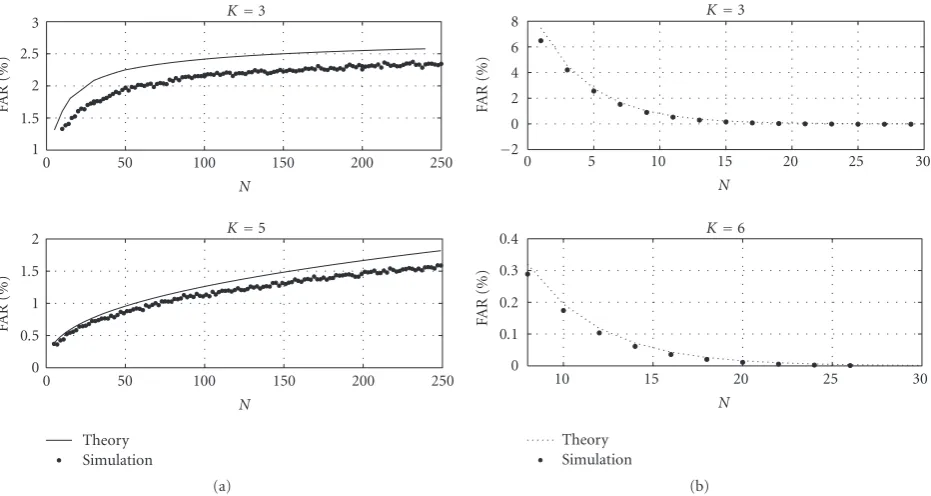
The accuracy of this method is tested using simulation. A comparison of the approximate FARs obtained from (20) with the FARs obtained from simulation for the AIC and MDL are shown in Figures4(a)and4(b), respectively. The FARs for two different array sizes as a function of N are analyzed in both figures. Smaller values ofKare used for the MDL due to the fact that the FARs forK > 6 are less than 1/100 of 1%, which is too small to be computed reliably with
Table2: Estimated Error in TW Approximated AIC FARs forM=
0.
Mean Absolute Difference in FARs
Mean Relative Difference in FARs K
3 0.36% 18%
5 0.23% 14%
7 0.16% 11.5%
9 0.13% 10.3%
the TW distribution used in our analysis. A smaller range forN is also used for the MDL, as it is found to converge to zero very rapidly. For each value ofK andN, 106 Monte-Carlo simulations were run using complex white noise. The covariance matrix and its eigenvalues are computed and substituted into (10) to determine the number of sources that minimize the IC. The percentage of these runs for which
M >0 is the estimated FAR forM=0.
As Figures4(a)and4(b)show, the theoretically predicted FAR using the TW law provides a good estimate of the com-puted FAR whenM = 0 for both the AIC and MDL. Both figures suggest that the TW FAR estimate is an upper bound on the true FAR. This finding is a direct consequence of
Observation 2. AsKincreases, the approximation to the FAR
improves, which is a direct consequence of Observation 3. The agreement between the FARs obtained from theory and simulation is better for the MDL than for the AIC. This is due to the fact that the FARs are smaller for the MDL than the AIC, hence byObservation 4, this result is also expected. To obtain a more quantitative understanding of the discrepancy between the theory and simulation for AIC, we computed the mean absolute and relative difference between the FAR obtained from simulation and theory.Table 2compares these differences between the theoretical and simulated FARs for
K = 3, 5, 7, and 9 with N going from 2K − 3 up to
250.Table 2shows that both absolute and relative differences
uniformly decrease asKincreases.
4.3. Estimation of the IC FAR for M = 1. The FAR approximation from (14) is also valid for M = 1. Using the FAR approximation forM = 1 and repeating the same arguments for theM=0 case, it can be shown that the FAR atM=1 can be approximated as
PFA(1)≈P
λ2>Λ2|1
, (21)
whereΛ2is the solution to the equation 1 + ln(λ2)−λ2+
2γIC(K −1)/N = 0. The solution for Λ2 can be found
numerically with the same method used for Λ1 with the
M=0 case.
The difference between the analysis of the M = 0 and
M = 1 cases lies in the way we determine the probability of the events on the right-hand sides of (18) and (21). The probability of the eventλ1 >Λ1can be estimated using the
TW distribution. However, the TW law is not applicable to estimating the probability of the eventλ2 > Λ2 because it
1 1.5 2 2.5 3
FA
R
(%
)
0 50 100 150 200 250
N K=3
0 0.5 1 1.5 2
FA
R
(%
)
0 50 100 150 200 250
N K=5
Theory Simulation
(a)
−2 0 2 4 6 8
FA
R
(%
)
0 5 10 15 20 25 30
N K=3
0 0.1 0.2 0.3 0.4
FA
R
(%
)
10 15 20 25 30
N K=6
Theory Simulation
(b)
Figure4: (a) (plates on left) AIC FAR for different array sizes as a function of sample size with no sources present. (b) (plates on right) MDL
FAR for different array sizes as a function of sample size with no sources present.
A hypothesis test for the presence ofMsources, however, can be constructed using the TW distribution based on the following theorem (whose proof is given in [16, pages 303 and 321]).
Eigenvalue Inclusion Principle. Let λ[MM,K+1] denote the (M+
1)th largest sample eigenvalue of aK×Kcovariance matrix constructed from the output signal from aK element array containing M sources (where M < K and the sources are as described earlier) along with noise ∼ NC(0, 1). Let
λ[1]0,K−Mdenote the largest eigenvalue of a (K−M)×(K−M)
covariance matrix constructed from the output signal from a
K−Melement array containing zero sources and only noise
∼NC(0, 1).Then it follows that:
Pλ[MM+1],K ≥x
≤Pλ[1]0,K−M ≥x
∀x∈R. (22)
This theorem essentially relates the CDF for the largest noise eigenvalue from aK element array havingMsources with the CDF for the largest eigenvalue from a “noise” covariance matrix for a (K−M) element array. For the case of
M =1, the eigenvalue inclusion theorem and (21) imply an upper bound on the FAR forM =1that can be expressed in terms of the largest eigenvalue of a noise covariance matrix:
PFA(1)≈P
λ2>Λ2|1
,
Pλ[2]1,K≥x
≤Pλ[1]0,K−1≥x
=⇒PFA(1)≤P
λ[1]0,K−1>Λ2
.
(23)
The probability of the event on the right-hand side of (23) now can be estimated using the TW law, since it involves the largest eigenvalue of a covariance matrix containing no sources. Proceeding as before with theM=0 case, this upper bound can be expressed in terms of the TW CDF as
PFA(1)≤1−P
F2
Λ2−μK−1,N
σK−1,N
. (24)
Our analysis supports the conjecture that a single source will “pull up” the largest noise eigenvalue as the source’s power increases [16]. Figure 5 shows the simulated FARs for the AIC (top panel) and MDL (lower panel) for an input from a 3-element ULA containing a single source. The FARs are computed as a function of the sample size, where for each N, estimates are obtained from 105 Monte-Carlo
simulations. The simulations were run at different signal to noise ratios (SNR) for the source. Figure 5 shows that as the SNR increases, the FAR also increases and approaches an upper limit. From (21), this implies that as the SNR increases, the distribution for the second largest eigenvalue shifts to larger values. From (22), we know the second largest eigenvalue’s distribution is bounded above as the source power becomes asymptotically large.
Figure 6compares the upper bound for the FAR obtained
0 0.5 1 1.5 2
FA
R
(%
)
0 50 100 150 200 250
N AIC
(a)
0 0.001 0.01 0.1 1 2.5
log
10
(F
AR)
(%)
5 10 15 20 25 30
N MDL
SNR=40 dB SNR=0 dB
SNR= −6 dB SNR= −12 dB (b)
Figure5: Estimated FARs for a single source from a 3-element ULA
as a function of the number of samples.
principle overestimates the true FAR since it replaces the probability of the event of interest (λ[2]1,K ≥ Λ2), with an
event (λ[1]0,K−1 ≥ Λ2), whose probability is larger. Second,
Observation 2shows that the use of the TW law in evaluating
the probability of the event (λ[1]0,K−1≥Λ2) gives a probability
slightly larger than the true probability. The bottom panel in
Figure 6compares the estimated upper bound for the FAR
with that obtained using the eigenvalue inclusion principle and the TW distribution for the MDL. The FARs for the MDL are compared for two different array sizes ofK = 3 andK =6.Similar to the AIC, the MDL results also show that the agreement between the TW and the true largest noise sample eigenvalue improves asKincreases, as expected from
Observation 3. ForK = 6, in fact, the two estimated and
TW derived FARs are seen to be practically identical. This is again consistent withObservation 4, which suggests that the agreement of the TW and largest noise eigenvalue CDFs improves for events lying further out in the distribution’s right-tail.
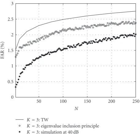
The results fromFigure 6raise the question of which one of the two overestimation factors is the dominant one. If the eigenvalue inclusion theorem produced a very tight upper bound and the majority of the overestimation was due to TW distribution approximation, then this would suggest a possi-ble means of improving the upper bounds through the use of correction factors to the approximate distribution function. To obtain an understanding of the relative importance of the two overestimation factors,Figure 7replotted the FARs for the AIC inFigure 6 forK = 3.Additionally, Figure 7
also plotted the FAR derived from the eigenvalue inclusion principle using (23). The FAR obtained using the eigenvalue
0 0.5 1 1.5 2 2.5 3
FA
R
(%
)
0 50 100 150 200 250
N AIC
(a)
−3 −2 −1 0 1
log
10
(F
AR)
(%)
0 10 20 30 40 50 60
N MDL
K=3: TW K=6: TW
K=3: simulation at SNR=40 dB K=6: simulation at SNR=40 dB (b)
Figure6: Comparison of TW FAR Upper Bound with Estimated
FAR Upper Bound.
0 0.5 1 1.5 2 2.5 3
FA
R
(%
)
50 100 150 200 250
N
K=3: TW
K=3: eigenvalue inclusion principle K=3: simulation at 40 dB
Figure7: Contributions to the Overestimation in the FAR of the
AIC.
5. Conclusions
Information-theoretic methods for model selection are perhaps the most commonly used means for source enu-meration in signal processing. The implementation of these methods, however, requires the use of large sample approx-imations, thereby calling into question the performance of these methods for small sample sizes [1, 5]. As discussed in the introduction, past performance analyses either have relied on the use of large sample size assumptions, and large array sizes, or are computationally complicated and expensive to use. In this paper, we presented a simple, computationally efficient method for FAR estimation using a recent development from random matrix theory known as the Tracy-Widom (TW) law.
The TW law was introduced as a simple means of approximating the distribution for the largest eigenvalue of a covariance matrix from the output signal of an array containing only white noise. It was shown that the TW law allows the largest sample eigenvalue to be expressed in a standardized form whose distribution is independent of the sample size or array size. For a wide range of array and sample sizes, it was shown that the TW distribution approximates the right-hand tail of the true distribution for the largest sample eigenvalue to within 1%. These results set the TW distribution apart from other distributions used for the largest noise eigenvalue, which are either based on large sample sizes [17], require the use of lookup tables that are functions of bothKandN[18], or are numerically difficult to evaluate [19].
We analyzed the performance of the AIC and MDL for small sample sizes under the condition that the noise variance is known. A general information criterion appli-cable to both the MDL and AIC was derived under this condition. Using the approximation that the FAR for M
sources can be estimated as the probability of the single event that the IC estimates M + 1 sources present, we derived the criteria for FAR when M = 0 and when
M = 1 in terms of the sample eigenvalues. It was shown that the FAR for M = 0 could be approximated as the probability that the largest noise eigenvalue exceeded a critical value. The critical value was the zero of a nonlinear equation having one real root, and its value could easily be obtained numerically. In this case, the FAR could be directly estimated using the TW distribution. Because the TW predicted FARs were always overestimates of the true FAR, the FARs obtained using the TW distribution will be conservative estimates of the true FAR. Our computation and simulation results demonstrate that the agreement between the estimated FAR using the TW distribution and with the simulated FARs improved uniformly with increasingK.The TW approximated FAR and the FAR estimated by simulation showed better agreement with the MDL than for the AIC. This was due in part to the fact that the FARs for the MDL were smaller than the AIC and could therefore be better approximated using the TW distribution.
For the case where there is one external source in the receiver input (M=1), an estimate for the FAR was derived based on the eigenvalue inclusion principle. It was shown
that the eigenvalue inclusion principle and the use of the TW distribution both contribute to the overestimation in the FAR. Thus, FAR estimates obtained with the TW distribution when sources are present will always be upper bounds for the true FAR. Similar to the FAR for theM=0 case, it was shown that this upper bound becomes uniformly tighter as the array size increases. For the AIC, for example, it was shown that as the array size increased fromK = 3 toK = 9, the relative difference between the true and upper bound FAR uniformly decreased from 20% to 10%.
Recent developments in random matrix theory should allow for further improvements in the FAR estimates using the TW law and also the possibility that the TW law can be used to estimate missed detection probabilities. Recent analyses have shown that the TW law can be generalized to non-central white Wishart distributions using a standardized test statistic similar to that used in the TW distribution for white Wishart distributions [29,30]. There is evidence based on empirical studies in the engineering literature [12] that support the notion that such an approach is possible. These results, while still preliminary, would allow the TW law to be extended so that it could be directly applied to signal eigenvalues and not just noise eigenvalues, thereby making the use of the eigenvalue inclusion principle unnecessary. Since the use of eigenvalue inclusion principle artificially inflates the FAR estimates obtained, this approach would produce tighter bounds for the FAR and also allow for more precise statistical analyses.
Acknowledgments
This project is supported by AFOSR Grant # FA9550-05-1-0035. Partial funding support was also provided by AFRL, Reference Systems Branch, WPAFB. The authors thank Dr. Steven E. Wright, Professor in the Mathematics department at Miami University for his suggestion on the use of complex Stiefel manifolds to determine the number of free model parameters.
References
[1] D. J. Navarro, “A note on the applied use of MDL approxi-mations,”Neural Computation, vol. 16, no. 9, pp. 1763–1768, 2004.
[2] H. Akaike, “A new look at the statistical model identification,”
IEEE Transactions on Automatic Control, vol. 19, no. 6, pp. 716–723, 1974.
[3] Y. Sakamoto, M. Ishiguro, and G. Kitagawa,Akaike Informa-tion Criterion Statistics, KTK Scientific, Tokyo, Japan, 1986. [4] J. Rissanen, “A universal prior for integers and estimation by
minimal discription length,”The Annals of Statistics, vol. 11, no. 2, pp. 416–431, 1983.
[5] P. Grunwald,The Minimum Description Length Principle, The MIT Press, Cambridge, Mass, USA, 2007.
[7] M. S. Bartlett, “A note on the multiplying factors for various χ2distributions,”Journal of the Royal Statistical Society. Series
B, vol. 16, no. 2, pp. 296–298, 1954.
[8] Q. Wu and D. R. Fuhrmann, “A parametric method for determining the number of signals in narrow-band direction finding,”IEEE Transactions on Signal Processing, vol. 39, no. 8, pp. 1848–1857, 1991.
[9] M. Wax and T. Kailath, “Detection of signals by information theoretic criteria,”IEEE Transactions on Acoustics, Speech, and Signal Processing, vol. 33, no. 2, pp. 387–392, 1985.
[10] H. Wang and M. Kaveh, “On the performance of signal-subspace processing—part I: narrow-band systems,” IEEE Transactions on Acoustics, Speech, and Signal Processing, vol. 34, no. 5, pp. 1201–1209, 1986.
[11] K. M. Wong, Q.-T. Zhang, J. P. Reilly, and P. C. Yip, “On information theoretic criteria for determining the number of signals in high resolution array processing,”IEEE Transactions on Acoustics, Speech, and Signal Processing, vol. 38, no. 11, pp. 1959–1971, 1990.
[12] M. Kaveh, H. Wang, and H. Hung, “On the theoretical performance of a class of estimators of the number of narrowband sources,”IEEE Transactions on Acoustics, Speech, and Signal Processing, vol. 35, no. 9, pp. 1350–1352, 1987. [13] V. T. Ermolaev, A. A. Mal’tsev, and K. V. Rodyushkin,
“Statistical characteristics of the AIC and MDL criteria in the problem of estimating the number of multivariate signals in the case of a short sample,” Radiophysics and Quantum Electronics, vol. 44, no. 12, pp. 977–983, 2001.
[14] C. A. Tracy and H. Widom, “On orthogonal and symplectic matrix ensembles,”Communications in Mathematical Physics, vol. 177, no. 3, pp. 727–754, 1996.
[15] K. Johansson, “Shape fluctuations and random matrices,”
Communications in Mathematical Physics, vol. 209, no. 2, pp. 437–476, 2000.
[16] I. M. Johnstone, “On the distribution of the largest eigenvalue in principal components analysis,”The Annals of Statistics, vol. 29, no. 2, pp. 295–327, 2001.
[17] C. G. Khatri, “Distribution of the largest or the smallest characteristic root under null hypethesis concerning complex multivariate normal populations,”The Annals of Mathematical Statistics, vol. 35, no. 4, pp. 1807–1810, 1964.
[18] K. C. S. Pillai and D. L. Young, “An approximation to the distribution of the largest root of a matrix in complex multivariate analysis,” Tech. Rep., Department of Statistics, Purdue University, West Lafayette, Ind, USA, 1969.
[19] V. T. Ermolaev and K. V. Rodyushkin, “The distribution function of the maximum eigenvalue of a sample correlation matrix of internal noise of antenna-array elements,” Radio-physics and Quantum Electronics, vol. 42, no. 5, pp. 439–444, 1999.
[20] D. M. Boroson, “Sample size considerations for adaptive arrays,”IEEE Transactions on Aerospace and Electronic Systems, vol. 16, no. 4, pp. 446–451, 1980.
[21] F. J. Dyson, “Statistical theory of energy levels of complex systems—part 1,”Journal of Mathematical Physics, vol. 3, pp. 140–175, 1962.
[22] A. Bejan,Largest eigenvalues and sample covariance matrices, M.S. dissertation, Department of Statistics, The University of Warwick, 2005.
[23] A. Bejan, “Tracy-Widom and Painleve II : computational aspects and realization in S-Plus,” inProceedings of the 14th
Conference on Applied and Industrial Mathematics (ICM ’06), Chisinau, Moldova, 2006.
[24] S. Geman, “A limit theorem for the norm of random matrices,”
Annals of Probability, vol. 8, no. 2, pp. 252–261, 1980. [25] T. R. Kn¨osche, E. M. Berends, H. R. A. Jagers, and M. J. Peters,
“Determining the number of independent sources of the EEG: a simulation study on information criteria,”Brain Topography, vol. 11, no. 2, pp. 111–124, 1998.
[26] K. Harmanci, J. Tabrikian, and J. L. Krolik, “Relationships between adaptive minimum variance beamforming and opti-mal source localization,”IEEE Transactions on Signal Process-ing, vol. 48, no. 1, pp. 1–12, 2000.
[27] D. B. Fuchs, O. Y. Viro, S. P. Novikov, and V. A. Rokhlin,
Topology II: Homotopy and Homology. Classical Manifolds, vol. 2, Springer, Berlin, Germany, 2003.
[28] Q.-T. Zhang, K. M. Wong, P. C. Yip, and J. P. Reilly, “Statistical analysis of the performance of information theoretic criteria in the detection of the number of signals in array processing,”
IEEE Transactions on Acoustics, Speech, and Signal Processing, vol. 37, no. 10, pp. 1557–1567, 1989.
[29] N. El Karoui, “Recent results about the largest eigenvalue of random covariance matrices and statistical application,”Acta Physica Polonica B, vol. 36, no. 9, pp. 2681–2697, 2005. [30] N. El Karoui, “Tracy-widom limit for the largest eigenvalue of