Stochastic Simulation of the Kinetics of Multiple Interacting Nucleic Acid Strands

(1)

Nucleic Acid Strands

Thesis by

Joseph Malcolm Schaeffer

In Partial Fulfillment of the Requirements

for the Degree of

Doctor of Philosophy

California Institute of Technology

Pasadena, California

2013

(2)

c

2013

Joseph Malcolm Schaeffer

(3)

Acknowledgements

Thanks to my advisor Erik Winfree, for his enthusiasm, expertise, and encouragement.

The models presented here are due in a large part to helpful discussions with Niles Pierce,

Robert Dirks, Justin Bois, and Victor Beck. Two undergraduates, Chris Berlind and Joshua

Loving, did summer research projects based on Multistrand and in the process helped

build and shape the simulator. There are many people who have used Multistrand and

provided very helpful feedback for improving the simulator, especially Josh Bishop, Nadine

Dabby, Jonathan Othmer, and Niranjan Srinivas. Nadine Dabby was also invaluable for

her feedback and discussions while writing the thesis. Thanks also to the many past and

current members of the DNA and Natural Algorithms group for providing a stimulating

environment in which to work.

Funding for this work was provided by National Science Foundation grants DMS-0506468

and CCF-0832824, and the Gordon and Betty Moore Foundation through the Caltech

Pro-grammable Molecular Technology Initiative.

There are many medical professionals to which I owe my good health while writing this

thesis, especially Dr. Jeanette Butler, Dr. Mariel Tourani, Cathy Evaristo, and the staff of

the Caltech Health Center, especially Alice, Divina, and Jeannie.

I want to acknowledge all my family and friends for their support. A journey is made

all the richer for having good company, and I would not have made it nearly as far without

all the encouragement.

Finally, I must thank my wife Lorian, who has been with me every step of this journey

(4)

Abstract

DNA nanotechnology is an emerging field which utilizes the unique structural properties of

nucleic acids in order to build nanoscale devices, such as logic gates, motors, walkers, and

algorithmic structures. Predicting the structure and interactions of a DNA device requires

good modeling of both the thermodynamics and the kinetics of the DNA strands within

the system. The kinetics of a set of DNA strands can be modeled as a continuous time

Markov process through the state space of all secondary structures. The primary means

of exploring the kinetics of a DNA system is by simulating trajectories through the state

space and aggregating data over many such trajectories.

We expand on previous work by extending the thermodynamics and kinetics models to

handle multiple strands in a fixed volume, and show that the new models are consistent

with previous models. We developed data structures and algorithms that allow us to take

advantage of local properties of secondary structure, improving the efficiency of the

sim-ulator so that we can handle larger systems. The new kinetic parameters in our model

were calibrated by analyzing simulator results on experimental systems that measure basic

kinetic rates of various processes. Finally, we apply the new simulator to explore a case

(5)

List of Figures

3.1 Secondary Structure Loop Decomposition . . . 9

4.1 Adjacent Microstate Diagram . . . 14

6.1 Representation of Secondary Structures . . . 34

6.2 Move Data Structure . . . 36

6.3 Move Update Example . . . 39

6.4 Move Generation Example . . . 41

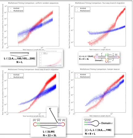
6.5 Full Comparison vs Kinfold 1.0 . . . 43

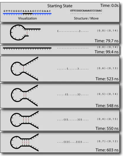
7.1 Trajectory Data . . . 46

7.2 Three-Way Branch Migration System . . . 47

7.3 Trajectory Output after 0.01 s Simulated Time . . . 48

7.4 Trajectory Output after 0.05 s Simulated Time . . . 49

7.5 Example Macrostate . . . 52

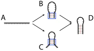
7.6 Hairpin Folding Pathways . . . 55

7.7 First Passage Time Data, Design B . . . 60

7.8 First Passage Time Data, Design A . . . 62

7.9 First Passage Time Data, Sequence Design Comparison . . . 62

7.10 First Passage Time Data, 6 Base Toeholds . . . 63

7.11 Starting Complexes and Strand Labels . . . 65

7.12 Final Complexes and Strand Labels . . . 65

8.1 Zippering Mechanism . . . 72

9.1 Four-Way Branch Migration Mechanism . . . 80

(9)

9.3 Four-Way Branch Migration Mechanism, Start and Stop States . . . 82

9.4 Bimolecular Success Rate vs Total Toehold Length . . . 84

9.5 Comparison of Experimental and Simulated Rates for Toehold Mediated Four-Way Branch Migration . . . 85

A.1 Polymer Graph Representation . . . 87

A.2 Polymer Graph Changes (Break Move) . . . 88

(10)

List of Tables

7.1 Two Branch Migration Sequences . . . 48

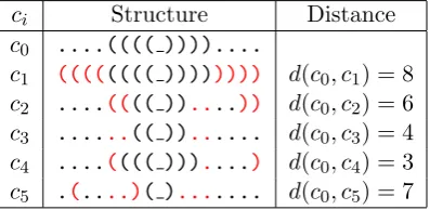
7.2 Distance Metric Examples . . . 53

7.3 Transition States in Hairpin Pathway . . . 56

7.4 Transition Pathways via Transition Mode Simulation . . . 57

7.5 Transition Pathway Statistics . . . 57

7.6 Transition Pathway Statistics, 100 Trajectories . . . 58

7.7 First Passage Time Data . . . 60

8.1 Average f(∆Gstep) for Forward Zippering Steps . . . 72

8.2 Calibratedkuni Parameters . . . 73

8.3 Bimolecular Association Rate khyb Parameters . . . 74

8.4 Calibratedkbi Parameters . . . 75

8.5 Comparison of Calibrated Parameters . . . 78

9.1 Sequences for Four-Way Branch Migration Domains . . . 83

(11)

Chapter 1

Introduction

DNA nanotechnology is an emerging field that utilizes the unique structural properties of

nu-cleic acids in order to build nanoscale devices, such as logic gates [23], motors [4, 1], walkers

[24, 1, 26], and algorithmic structures [18, 31]. These devices are built out of DNA strands

whose sequences have been carefully designed in order to control their secondary structure—

the hydrogen bonding state of the bases within the strand (called “base-pairing”). This

base-pairing is used to not only control the physical structure of the device, but also to

en-able specific interactions between different components of the system, such as allowing, for

example, a DNA walker to take steps along a prefabricated track. Predicting the structure

and interactions of a DNA device requires good modeling of both the thermodynamics and

the kinetics of the DNA strands within the system. Thermodynamic models can be used

to make equilibrium predictions for these systems, allowing us to look at questions like “Is

the walker-track interaction a well-formed and stable molecular structure?”, while kinetics

models allow us to predict the non-equilibrium dynamics, such as “How quickly will the

walker take a step?” While the thermodynamics of multiple interacting DNA strands is a

well-studied model [6], which allows for both analysis and design of DNA devices [34, 7],

previous work on secondary structure kinetics models only explored the kinetics of how a

single strand folds on itself [8].

The kinetics of a set of DNA strands can be modeled as a continuous time Markov

pro-cess through the state space of all secondary structures. Due to the exponential size of this

state space it is computationally intractable to obtain an analytic solution for most problem

sizes of interest. Thus the primary means of exploring the kinetics of a DNA system is by

simulating trajectories through the state space and aggregating data over many such

(12)

work [8] by using the multiple strand thermodynamics model [6] (a core component for

cal-culating transition rates in the kinetics model), adding new terms to the thermodynamics

model to account for stochastic modeling considerations, and by adding new kinetic moves

that allow bimolecular interactions between strands. Furthermore, we prove that this new

kinetics and thermodynamics model is consistent with the prior work on multiple strand

thermodynamics models [6].

The Multistrand simulator is based on the Gillespie algorithm [9] for generating sta-tistically correct trajectories of a stochastic Markov process. We developed data structures

and algorithms that take advantage of local properties of secondary structures. These

algo-rithms enable the efficient reuse of the basic objects that form the system, such that only a

very small part of the state’s neighborhood information needs to be recalculated with every

step. A key addition was the implementation of algorithms to handle the new kinetic steps

that occur between different DNA strands, without increasing the time complexity of the

overall simulation. These improvements lead to a reduction in worst case time complexity

of a single step and also led to additional improvements in the average case time complexity.

What data does the simulation produce? At the very simplest, the simulation produces

a full kinetic trajectory through the state space—the exact states it passed through, and

the time at which it reached them. A small system might produce trajectories that pass

through hundreds of thousands of states, and that number increases rapidly as the system

gets larger. Going back to our original question, the type of information a researcher hopes

to get out of the data could be very simple: “How quickly does the walker take a step?”,

with the implied question of whether it’s worth it to actually purchase the particular DNA

strands composing the walker to perform an experiment, or go back to the drawing board

and redesign the device. One way to acquire that type of information is to look at the first

time in the trajectory where we reached the “walker took a step” state, and record that

information for a large number of simulated trajectories in order to obtain a useful answer.

We designed and implemented new simulation modes that allow the full trajectory data to

be condensed as it’s generated into only the pieces the user cares about for their particular

question. This analysis tool also required the development of flexible ways to talk about

states that occur in trajectory data; if someone wants data on when the walker took a step,

we have to be able to express that in terms of the Markov process states which meet that

(13)

Chapters 1, 2, 3, 4, 6, 7, and Appendix A originally appeared in my Master’s thesis.

Chapter 5 is a completely new proof of equivalence between the thermodynamics model we

develop in Chapter 3 and the NUPACK model. Chapter 8 discusses how we calibrate the

kinetics parameters kuni and kbi which were introduced in Chapter 4. Chapter 9 is a case

study on using the simulator to explore a toehold-mediated four-way branch migration. The

experimental data kf it₁ in Chapter 9 is from Dabby, et al. [5] on which I am a co-author.

I performed simulations using Multistrand for that work, which appear in that paper and

are presented in more detail here.

Found in the Master’s thesis but not here are two appendices which describe the software

design for the data structures and algorithms used in simulator, as well as a different proof

(14)

Chapter 2

System

We are interested in simulating nucleic acid molecules (DNA or RNA) in a stochastic regime;

that is to say that we have a discrete number of molecules in a fixed volume. This regime is

found in experimental systems that have a small volume with a fixed count of each molecule

present, such as the interior of a cell. We can also apply this to experimental systems with

a larger volume (such as a test tube) when the system is well mixed, as we can pick a fixed

(small) volume and deal with the expected counts of each molecule within it, rather than

the whole test tube.

To discuss the modeling and simulation of the system, we need to be very careful to

define the components of the system, and what comprises a state of the system within the

simulation.

2.1

Strands

Each DNA molecule to be simulated is represented by a strand. Our system then contains

a set of strands Ψ∗, where each strand s ∈ Ψ∗ is defined by s = (id, label, sequence). A strand’siduniquely identifies the strand within the system, while thesequenceis the ordered

list of nucleotides that compose the strand.

Two strands could be considered identicalif they have the same sequence. However, in

some cases it is convenient to make a distinction between strands with identical sequences.

For example, if one strand were to be labeled with a fluorophore, it would no longer be

physically identical to another with the same sequence but no fluorophore. Thus, thelabel

is used to designate whether two strands are identical. We define two strands as being

(15)

the label and the sequence is not used, so it will be explicitly noted when it is important.

2.2

Complex Microstate

Acomplexis a set of strands connected by base pairing (secondary structure). We define the

state of a complex byc= (ST, π∗, BP), called the “complex microstate”. The components are a nonempty set of strands ST ⊆Ψ∗, an ordering π∗ on the strands ST, and a list of base pairingsBP ={(ij·kl)| baseion strandj is paired to basek on strandl, and j≤l,

withi < k ifj=l}, where we note that “strandl” refers to the strand occurring in position

lin the orderingπ∗. Note that we require a complex to be “connected”: there is no proper subset of strands in the complex for which the base pairings involving those strands do not

involve at least one base outside that subset. Given a complex microstate c, we will use ST(c), π∗(c), BP(c) to refer to the individual components.

While this definition defines the full space of complex microstates, it is common to

disal-low some secondary structures due to physical or computational constraints. For example,

we disallow the pairing of a base with any other within three bases on the same strand, as

this would correspond to an impossible physical configuration. Another class of disallowed

structures are called thepseudoknottedsecondary structures, which require computationally

difficult energy model calculations, and are fully defined and discussed further in Appendix

A.

2.3

System Microstate

A system microstate represents the configuration of the strands in the volume we are

sim-ulating (the “box”). Since we allow complexes to be formed of one or more strands, every

unique strand in the system must be present in a single complex and thus we can represent

the system microstate by a set of those complexes.

We define a system microstate ias a set of complex microstates, such that each strand in the system is in exactly one complex within the system. This is formally stated in the

(16)

[

c∈i

ST(c) = Ψ∗ and ∀c, c0 ∈iwithc6=c0, ST(c)∩ST(c0) =∅ (2.1)

(17)

Chapter 3

Energy

The conformation of a nucleic acid strand at equilibrium can be predicted by a well-studied

model, called the nearest neighbor energy model [20, 19, 21]. Recent work has extended

this model to cover systems with multiple interacting nucleic acid strands [6].

The distribution of system microstates at equilibrium is a Boltzmann distribution, where

the probability of observing a microstate iis given by

P r(i) = 1 Qkin

∗e−∆Gbox(i)/RT _(3.1)

where ∆Gbox(i) is the free energy of the system microstate i, and is the key quantity

determined by these energy models. Qkin =

P

ie

−∆Gbox(i)/RT _{is the partition function of}

the system,R is the gas constant, andT is the temperature of the system.

3.1

Energy of a System Microstate

We now consider the energy of the system microstatei, and break it down into components. The system consists of many complex microstates c, each with their own energy. We also

must account for the entropy of the system (the number of configurations of the complexes

spatially within the “box”) in the energy, and thus must define these two terms.

Let us first consider the entropy term. We consider the “zero” energy system microstate

to be the one in which all strands are in separate complexes, thus our entropy term is in

(18)

We assume that the number of complexes in the system, C, is much smaller than the number of states within our box,_VV

0, whereV is the simulated volume, andV0is our reference volume1 chosen to be consistent with existing thermodynamic models (see Sections 3.4 and

5).

We can then approximate the standard statistical entropy of the system asC∗RTlog_VV 0. Letting Ltot be the total number of strands in the system, our zero state is then Ltot ∗

RTlog_VV

0. Defining ∆Gvolume = RTlog

V

V0, the contribution to the energy of the system microstateifrom the entropy of the box is then:

(Ltot−C)∗∆Gvolume

And thus in terms of C, Ltot,∆Gvolume and ∆G(c) (the energy of complex microstatec,

defined in the next section), we define ∆Gbox(i), the energy of the system microstate i, as

follows:

∆Gbox(i) = (Ltot−C)∗∆Gvolume+

X

c∈i

∆G(c)

The energy formulas derived here, suitable for our stochastic model, differ from those in

[6] in two main ways: the lack of symmetry terms, and the addition of the ∆Gvolume term.

We compare this stochastic model to the mass action model in much more detail in Section 5.

3.2

Energy of a Complex Microstate

We previously defined a complex microstate in terms of the list of base pairings present

within it. However, the well-studied models are based upon nearest neighbor interactions

between the nucleic acid bases. These interactions divide the secondary structure of the

1

We calculateV0as the volume in which we would have exactly one molecule at a standard concentration of 1 mol/L:V0= 1/(Na∗1 mol/L), whereNa is Avogadro’s number, and thusV0 is in liters.

Similarly, we may wish to calculateV based on the concentrationuin mol/L of a single strand such that the volume V is chosen such that exactly one molecule is present in that volume. In this case we have

V =_u∗N1

a and our number of states in the box is then

V V0 =

Na

u∗Na =

1

(19)

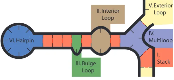
system into local components which we refer to asloops, shown in Figure 3.1.

IV. Multiloop V. Exterior

Loop

I. Stack III. Bulge

Loop

II. Interior Loop

VI. Hairpin

Figure 3.1: Secondary structure divided into loops

These loops can be broken down into different categories, and parameter tables and

formulas for each category have been determined from experimental data [21]. Each loop

l has an energy, ∆G(l) which can be retrieved from the appropriate parameter table for its category. Each complex also has an energy contribution associated with the entropic

initiation cost [3] (e.g., rotational) of bringing two strands together, ∆Gassoc, and the total

contribution is proportional to the number of strands L within the complex, as follows:

(L−1)∗∆Gassoc.

The energy of a complex microstatecis then the sum of these two types of contributions. We can also divide any free energy ∆G into the enthalpic and entropic components, ∆H

and ∆S related by ∆G = ∆H + T ∗∆S, where T is the temperature of the system. For a complex microstate, each loop can have both enthalpic and entropic components,

but ∆Gassoc is usually assumed to be purely entropic [20]. This becomes important when

determining the kinetic rates, in Section 4.

We use ∆G(c) to refer to the energy of a complex microstate to be consistent with the

nomenclature in [6], where ∆G(c) refers to the energy of a complex when all strands within

it are consider unique (as is the case in our system), and ∆G(c) is the energy of the

com-plex, without assuming that all strands are unique (and thus it must account for rotational

(20)

In summary, the standard free energy of a complex microstatec, containingL=|ST(c)| strands:

∆G(c) =

 

X

loop l∈c

∆G(l)



+ (L−1)∆Gassoc

3.3

Computational Considerations

While the simulator could use the system microstate energy in the form given in the previous

sections, it is convenient for us to group terms such that the computation need only take

place per complex. Thus we wish to include the (Ltot −C)∆Gvolume term in the energy

computation for the complex microstates. Recall that Ltot is the number of strands in the

system, andC is the number of complexes in the system microstate. Assuming that we are computing the energy ∆Gbox of system microstatei, we can rewriteLtot and C as follows:

Ltot =

X

c∈i

|ST(c)|

C = X

c∈i

1

And thus arrive at:

∆Gbox(i) =

X

c∈i

∆G(c) + (|ST(c)| −1)∗∆Gvolume

We then define ∆G∗(c) = ∆G(c) + (|ST(c)| −1)∗∆Gvolume, and L(c) = |ST(c)| and

thus have the following forms for the energy of a system microstate and the energy of a

(21)

∆Gbox(i) =

X

c∈i

∆G∗(c)

∆G∗(c) =

 

X

loop l∈c

∆G(l)



+ (L(c)−1)∗(∆Gassoc+ ∆Gvolume)

3.4

Choice of Units

The free energy ∆G◦ for a reaction A+B −₎*− C is usually expressed in terms of the equilibrium constant Keq and the concentrations [A],[B],[C] (in mol/L) of the molecules

involved, as follows: e∆G◦/RT = Keq = [A_[_C][B_]]. We can also express the free energy ∆G0

in terms of the dimensionless mole fractions xA, xB, xC, where xi = [i]/ρH2O (for dilute solutions), andρH2O is the molarity of water (55.14 mol/L at 37

◦_{C). In this case, we have}

e∆G0/RT =K_eq0 = xA∗xB

xC , and relating it to the previous equation, we see that e

∆G0/RT ₌

([A]/ρH₂O)∗([B]/ρH₂O)

[C]∗ρH₂O =

[A][B] [C] ∗

1

ρH₂O =e

∆G◦_/RT

∗e−logρH2O_{. Thus if we have an energy ∆G}◦

which was for concentration units and we wish to use mole fraction units, we must adjust it

by−RTlogρH2O(−2.47 kcal/mol at 37

◦_{C) to obtain the correct quantity. In general, if we}

have a complex ofN molecules, the conversion to mole fractions will require an adjustment of −(N−1)∗RTlogρH2O.

In the reference [6], free energies are always in mole fraction units, and the−RTlogρH2O term is included as part of the ∆Gassoc term (footnote 13 in [6]), as follows: ∆Gassoc =

∆Gpubassoc−RTlogρH2O, where ∆G

pub

assoc is the reference value found in [3] (1.96 kcal/mol at

37◦C) and is the value we use for ∆Gassoc when using molar concentration units.

Since we expect the probability of observing a particular complex microstate to remain

the same no matter what reference units we use for the free energy, this implies that if

we wanted to express our ∆G∗(c) in mole fraction units, we would need to use ∆Gassoc =

∆Gpubassoc−RTlogρH2Oand ∆Gvolume=RTlog

V

V0+RTlogρH2Oin order for the probability of observing the statecto remain the same. We note that this ∆Gvolume simplifies to being

∆Gvolume = RTlog(V ∗ ρH2O ∗Na) = RTlogMs, where Ms is the number of solvent molecules found in the volumeV.

We use the molar concentration units (∆Gvolume =RTlog_VV₀ = RTlog_u1, ∆Gassoc =

(22)

(23)

Chapter 4

Kinetics

4.1

Basics

Thermodynamic predictions have only limited use for some systems of interest, if the key

information to be gathered is the reaction rates and not the equilibrium states. Many

systems have well-defined ending states that can be found by thermodynamic prediction,

but predicting whether it will reach the end state in a reasonable amount of time requires

modeling the kinetics. Kinetic analysis can also help uncover poor sequence designs, such

as those with alternate reactions leading to the same states, or kinetic traps which prevent

an intended reaction from occurring quickly.

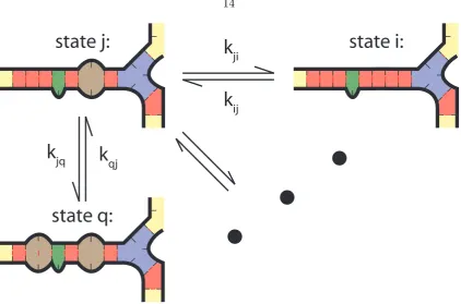
The kinetics are modeled as a continuous time Markov process over secondary structure

space. System microstates i, j are considered adjacent if they differ by a single base pair (Figure 4.1), and we choose the transition rates kij (the transition from state ito state j)

and kji such that they obey detailed balance:

kij

kji

=e−

∆_Gbox(j)−∆_Gbox(i)

RT (4.1)

This property ensures that given sufficient time we will arrive at the same equilibrium

state distribution as the thermodynamic prediction, (i.e., the Boltzmann distribution on

system microstates, equation 3.1) but it does not fully define the kinetics as this only

constrains the ratio kij

kji. We discuss how to choose these transition rates in the following

sections, but regardless of this choice, we can still determine how the next state is chosen

(24)

state j:

state i:

state q:

k

_ji

k

_ij

k

_qj

k

_jq

Figure 4.1: System microstatesi, q adjacent to current statej, with many others not shown

Given that we are currently in state i, the next state m in a simulated trajectory is

chosen randomly among the adjacent states j, weighted by the rate of transition to each.

P r(m) = kim Σjkij

(4.2)

Similarly, the time taken to transition to the next state is chosen randomly from an

exponential distribution with rate parameter λ, whereλis the total rate out of the current

state, Σjkij.

P r(∆t) =λexp(−λ∆t) (4.3)

We will now classify transitions into two exclusive types: those that change the number

of complexes present in the system, calledbimolecular transitions, and those where changes

(25)

4.2

Unimolecular Transitions

Because unimolecular transitions involve only a single complex, it is natural to define these

transitions in terms of the complex microstate which changed, rather than the full system

microstate. Like Figure 4.1 implies, we define a complex microstate das being adjacent to

a complex microstate c if it differs by exactly one base pair. We call a transition from c to d that adds a base pair a creation move, and a transition from c to d that removes a

base pair adeletionmove. The exclusion of pseudoknotted structures is not inherent in this

definition of adjacent states, but rather arises from our disallowing pseudoknotted complex

microstates.

In more formal terms we now define the adjacent states to a system microstate, rather

than those adjacent to a complex microstate as in the simple definition above. Recall from

Section 2.3 that |i|is the number of complexes present in system microstate i, andi\j is the set of complex microstates inithat are not also in system microstatej.

Two system microstates i, j are adjacent by a unimolecular transition iff ∃c ∈i, d ∈j such that:

|i|=|j|and i\j={c}and j\i={d} (4.4)

and one of these two holds:

BP(c)⊂BP(d) and |BP(d)|=|BP(c)|+ 1 (4.5)

BP(d)⊂BP(c) and |BP(c)|=|BP(d)|+ 1 (4.6)

In other words, the only differences between i and j are in c and d, and they differ by

exactly one base pair. If equation 4.5 is true, we call the transition fromi toj a base pair creation move, and if equation 4.6 is true, we call the transition from i to j a base pair

deletion move. Note that if itoj is a creation move, j toi must be a deletion move, and vice versa. Similarly, if there is no transition fromitoj, there cannot be a transition from

(26)

4.3

Bimolecular Transitions

A bimolecular transition from system microstateito system microstate j is one where the single base pair difference between them leads to a differing number of complexes within

each system microstate. This differing number of complexes could be due to a base pair

joining two complexes in i to form a single complex in j, which we will call a join move. Conversely, the removal of this base pair from icould cause one complex inito break into

two complexes withinj, which we will call abreak move. Note that ifitoj is a join move, thenj toimust be a break move, and vice versa. As we saw before, this also implies that

every bimolecular move is reversible.

Formally, a transition from system microstateito system microstate j is a join move if |i|=|j|+ 1 and we can find complex microstatesc, c0 ∈iand d∈j, with c6=c0 such that

the following equations hold:

i\ {c, c0}=j\ {d} (4.7)

∃x∈BP(d) s.t. BP(d)\ {x}=BP(c)∪BP(c0) (4.8)

Similarly, a transition from system microstate ito system microstatej is a break move if|i|+ 1 =|j|and we can find complex microstatesc∈iandd, d0∈j withd6=d0 such that the following equations hold:

i\ {c}=j\ {d, d0} (4.9)

∃x∈BP(c) s.t. BP(c)\ {x}=BP(d)∪BP(d0) (4.10)

While arbitrary bimolecular transitions are not inherently prevented from forming

pseu-doknots in this model, we again implicitly prevent them by using only complex microstates

(27)

4.4

Transition Rates

Now that we have defined all of the possible transitions between system microstates, we

must decide how to assign rates to each transition. We know that if there is a transition

from system microstate i to system microstate j with rate kij there must be a transition

from j toiwith rate kji which are related by:

kij

kji

=e−

RT (4.11)

This condition is known as detailed balance, and does not completely define the rates

kij, kji. Thus a key part of our model is the choice of rate method, the way we set the rates

of a pair of reactions so that they obey detailed balance.

While our simulator can use any arbitrary rate method we can describe, we would like

our choice to be physically realistic (i.e., accurate and predictive for experimental systems).

There are several rate methods found in the literature [11, 12, 36] which have been used for

kinetics models for single-stranded nucleic acids [8, 36] with various energy models. As a

start, we have implemented three of these simple rate methods which were previously used

in single base pair elementary step kinetics models for single stranded systems. In addition

we present a rate method for use in bimolecular transitions that is physically consistent

with both mass action and stochastic chemical kinetics. We verify that the kinetics model

(and thus our choice of rate method) have been correctly implemented by verifying that the

detailed balance condition holds (Section 7.1.2).

In order to maintain consistency with known thermodynamic models, each pair ofkij and

kji must satisfy detailed balance and thus their ratio is determined by the thermodynamic

model, but in principle each pair could be independently scaled by some arbitrary prefactor,

perhaps chosen to optimize agreement with experimental results on nucleic acid kinetics.

However, since the number of microstates is exponential, this leads to far more model

parameters (the prefactors) than is warranted by available experimental data. For the time

being, we limit ourselves to using only two scaling factors: kuni for use with unimolecular

(28)

4.5

Unimolecular Rate Models

The first rate model we will examine is the Kawasaki method [11]. This model has the

property that both “downhill” (energetically favorable) and uphill transitions scale directly

with the steepness of their slopes.

kij = kuni∗e−

2RT (4.12)

kji = kuni∗e−

∆_Gbox(i)−∆_Gbox(j)

2RT (4.13)

The second rate model under consideration is the Metropolis method [12]. In this model,

all downhill moves occur at the same fixed rate, and only the uphill moves scale with the

slope. This means that the maximum rate for any move is bounded, and in fact all downhill

moves occur at this rate. This is in direct contrast to the Kawasaki method, where there is

no bound on the maximum rate.

if ∆Gbox(i)>∆Gbox(j) then kij = 1∗kuni (4.14)

kji= kuni∗e−

∆_Gbox(i)−∆_Gbox(j)

RT (4.15)

otherwise, kij = kuni∗e−

RT (4.16)

kji= 1∗kuni (4.17)

Finally, the entropy/enthalpy method [36] uses the division of free energies into entropic

and enthalpic components to assign the transition rates in an intuitive manner: base pair

creation moves must overcome the entropic energy barrier to bring the bases into contact,

and base pair deletion moves must overcome the enthalpic energy barrier in order to break

(29)

ifitoj is a creation: kij = kuni∗e

∆_Sbox(j)−∆_Sbox(i)

R (4.18)

kji= kuni∗e−

∆_Hbox(i)−∆_Hbox(j)

RT (4.19)

otherwise, kij = kuni∗e−

∆_Hbox(j)−∆_Hbox(i)

RT (4.20)

kji= kuni∗e

∆_Sbox(i)−∆_Sbox(j)

R (4.21)

We note that the value of kuni that best fits experimental data is likely to be different

for all three models (see Section 8). Additionally, due to equations 4.5 and 4.6, the energies

of system microstates iand j, ∆Gbox(i) and ∆Gbox(j) differ in exactly one pair of complex

microstates c∈i, d∈j, and by exactly three loop terms in those complex microstates.

4.6

Bimolecular Rate Model

When dealing with moves that join or break complexes, we must consider the choice of how

to assign rates for each transition in a new light. In the particular situation of the join

move, where two molecules in a stochastic regime collide and form a base pair, this rate is

expected to be modeled by stochastic chemical kinetics.

Stochastic chemical kinetics theory [9] tells us that there should be a rate constantksuch

that the propensity of a particular bimolecular reaction between two speciesXandY should bek∗#X∗#Y /V, where #X and #Y are the number of copies ofX andY in the volume V. Since our simulation considers each strand to be unique, #X = #Y = 1, and thus we see the propensity should scale as 1/V. Recalling that ∆Gvolume =RTlog_VV₀ =RTlog_u1,

we see that we can obtain the 1/V scaling by letting the join rate be proportional to

e−∆Gvolume/RT_.

Thus, we arrive at the following rate method, and note that the choice of k (above) or our scalar termkbican be found by comparison to experiments measuring the hybridization

(30)

ifitoj is a complex join move: kij = kbi∗e

−∆_Gvolume

RT =k_bi∗ V0

V =kbi∗u (4.22) kji= kbi∗e−

∆_Gbox(i)−∆_Gbox(j)+∆_Gvolume

RT (4.23)

otherwise, kij = kbi∗e−

∆_Gbox(j)−∆_Gbox(i)+∆_Gvolume

RT (4.24)

kji= kbi∗e−

∆_Gvolume

RT (4.25)

We note that like the bimolecular case, equations 4.7–4.10 imply that the system

mi-crostatesiand j differ by exactly three loop terms in their complex microstates. However,

they also differ in the total number of complexes within each system microstate, such that

ifitoj is a join move, ∆Gbox(i)−∆Gbox(j) = ∆Gloops(i, j)−∆Gvolume−∆Gassoc, where

∆Gloops(i, j) represents the energy differences between i and j due to the three differing

loop terms in the complex microstates.

This formulation is convenient for simulation, as the join rates are then independent

of the resulting secondary structure. We could use the other choices for assigning rates

from 4.4, but they would require much more computation time. While the above model

is of course an approximation to the physical reality (albeit one which we believe at least

intuitively agrees with what we expect from stochastic chemical kinetics), if we later

deter-mine there is a better approximation we could use that instead, even if it cost us a bit in

computation time. One issue in the above model that we wish to revisit in the future is that

due to the rate being determined foreverypossible first base pair between two complexes, the overall rate for two complexes to bind (by a single base pair) is proportional roughly to

the square of the number of exposed nucleotides (although possibly only a linear subset is

(31)

Chapter 5

Thermodynamic Equivalence

Between the Multistrand and

NUPACK Models

5.1

Introduction

We now wish to compare the Multistrand thermodynamics model and that of NUPACK

[34], which is described in [6]. These two models are over very similar state spaces; in the

Multistrand model we look at system microstates of a fixed volume where all strands are

uniquely labeled, and in the NUPACK model the system has states in a fixed volume, but

the strands in the system are not necessarily unique. So a natural way to begin comparing

the two models is to look at the probability of “events” in the system, such as the probability

of observing a particular state in the NUPACK model and the equivalent system microstates

in the Multistrand model after the system has been run long enough to reach equilibrium.

In order to calculate these probabilities, the quantity of interest is the partition function

for these models.

Let us consider the partition function for our system:

Qkin=

X

s∈χ

e−∆G(s)/RT

where χ is the set of all possible unpseudoknotted system microstates for our fixed set

of unique strands in a box of volume V containing Ms solvent molecules. We would like

to show how this partition function Qkin relates to the partition function Qbox used in

(32)

Qbox is for a system where strands are considered identical if they have the same sequences

and thus have symmetry factors when computing the energy of a complex. Additionally,

Qboxaccounts for the energetics of the “box” (the volume in which the strands are present)

as part of the partition function itself, rather than in the energy of system states as is done

in our kinetic system.

In the Multistrand thermodynamics model, strands in the system are defined by three

pieces of information: a unique identifier, a label, and a sequence. In all of our previous

analysis, strands are always considered unique. However, in order to compare our system

with that of Dirks, et al. [6], we allow for the possibility of strands being considered

indistinguishableif they share the same label and sequence. This will allow us to establish

an equivalence between microstates in our model and those found in the thermodynamics

work. We call the combination of label and sequence a strand type, thus if two strands are

the same type, they are considered indistinguishable.

The thermodynamic partition function Qbox is expressed (at the lowest level) in terms

of partition functionsQj, which is the partition function over a single complex with typej

independent of volume. A complex type is a fixed set of strand types and counts of each

strand type, and represents a connected complex containing those strands (regardless of

their unique id), for example, a complex type might be{3∗A,2∗B}, where A and B are strand types. Thus the partition function over this complex type is the partition function

over all possible states of a single connected complex containing threeAstrands and twoB

strands in any order. We now wish to break down our partition function Qkin into smaller

components in a similar way.

One way to approach the division of Qkin into smaller components is to look at the

complex partition functions for a particular set of strands ids. For example, in a system

with three strands (regardless of their types), one way to write the partition function is as

follows:

(33)

where Q_r is the partition function over all complex microstates which involve the set r of unique strands. Continuing this example, we let our three strands{1,2,3}(where numbers indicate their unique ids) have types{A, A, B}, respectively. Now letQkin_j be the partition function over complex microstates of a complex type j which used a fixed set of unique

identifiers—e.g., Qkin_{_A_} is the partition function over all complex microstates which involve a single strand of type A, with a fixed identifier. Note that we distinguish this with the

superscript kin due to the canonical Qj being over complex states where strands may be

considered indistinguishable, as opposed to our complex microstates where all strands are

unique. So now Q{1} =Q{2}=Qkin{A}, and so on, so we can simplify our original breakdown

of the partition function as follows:

Qkin=

Qkin_{_A_}2∗Qkin_{_B_}+Qkin_{₂_∗_A_}∗Q_{kin_B_}+ 2∗Qkin_{_A,B_}∗Qkin_{_A_}+Qkin_{₂_∗_A,B_}

We now observe that two of the original terms in the expression for Qkin have been

collected into the single term 2∗Qkin_{_A,B_}∗Qkin_{_A_}. We could calculate the coefficient in front of the Qkin_{_A,B_}∗Qkin_{_A_} term by determining how many distinct ways we could assign unique strand identifiers to the A and B strands that would lead to complexes consistent with those complex types. In this case there are only two ways: the only strand of typeB (with

unique id 3) could be paired with either one of the two strands of typeA (with unique ids 1,2) to form the {A, B} complex, and then the other strand is in the single{A} complex.

In this proof, we will show how to relate theQkin_j to the canonicalQj, as well as how to

calculate the coefficient present in our Qkin summation for each term when using theQkinj

form, which amounts to counting the number of ways we could assign the unique strand ids

in such a way as to match the complex types present in each term.

5.2

Definitions

We previously introduced the set of (uniquely labeled) strands Ψ∗, let us now introduce the

equivalent for the set of strand types. Ψ0 is the set of strand types (also known as species)

(34)

a set of strand types and the number of each present in the connected complex. We note

that since our set of strands is finite, the set of complex types is also finite though it can

be quite large.

To keep track of which complex types are present in a system microstate, we introduce

the population vectorm ∈_N|Ψ|_{, where we note}

N=Z≥0. The population vector indicates the number of complexes of that type present in the system microstate. The initial

popula-tion vectorm0∈N|Ψ0|indicates how many of each type of strand are present in the system.

We relate the two by the strand matrix A∈_N|Ψ0_|×|_Ψ_|

, whose entriesAij correspond to the

number of strands of strand type iin complex typej. By our previous definition of strand complex, the columns ofAare distinct because each column specifies the number of strands

of each type present in the complex type j for that column. Thus, if we have a system which starts withm0 of each strand species, Λ ={m|Am=m0}is the set of all population vectors consistent with conservation of strand counts.

Since [6] uses mole fraction units for all energies (see discussion in Section 3.4), we use

the same units for ∆Gvolume and ∆Gassoc, thus we have:

∆Gvolume = RTlogMs

∆Gassoc = ∆Gpubassoc−RTlogρH2O = ∆G

assoc

where ∆Gassoc is the equivalent term used in [6].

5.3

Proof

5.3.1 Qkin

j and Qj

We know from [6] that Qj is defined as:

Qj =

X

π∈Πj

(35)

where Πj is the set of distinguishable orderings on the strand types present in complex type

j. E.g., ifjis a complex type with{3∗A,2∗B}, Π_j is{(A, A, A, B, B),(A, A, B, A, B)}as every other ordering is equivalent to one of these two via a cyclic permutation (a permutation

on objects such that the ordering would remain the same when laid out on a circle). Qj(π)

is then the partition function over all states Ωj(π) which have a particular indistinguishable

ordering π, as follows:

Qj(π) =

X

c∈Ωj(π)

exp(−∆G(c)/RT)

In this summation, we use the free energy of a complex state with (possibly)

indistin-guishable strands, and thus there is an extra energy term relating to the rotational symmetry

R(c), as described in [6] as the factorR(we distinguish here due to different units leading to

the prefactor beingRT rather thankT). This is related to our ∆G(c) described in Section 3.2 as follows:

∆G(c) =RTlogR(c) + ∆G(c) (5.1)

We now wish to examine Qkin

j and see how it relates to Qj.

Qkin_j = X

π∈Πj

X

c∈Ωj(π)

exp(−∆G∗(c)/RT) (5.2)

where Πj is the set of circular orderings on the strand identifiers present in complex type j,

Ωj(π) is the set of all complex microstates which have orderingπ, the complex microstate

energy ∆G∗(c) = ∆G(c) + (L(c)−1)∗∆Gvolume, and where L(c) is the total number of

strands in c.

For example, if our complex typej is{3∗A,2∗B}like before, and we are given the ids {1,2,3} as strand typeA, and {4,5}as strand typeB, then we have:

Πj = {{1,2,3,4,5}, {1,2,3,5,4}, {1,2,5,3,4}, {1,2,5,4,3},

{1,2,4,3,5}, {1,2,4,5,3}, {1,5,2,3,4}, {1,5,2,4,3}, {1,5,3,2,4}, {1,5,3,4,2}, {1,5,4,2,3}, {1,5,4,3,2}}

(36)

P

i∈Ψ0Aij (which is equivalent to L(c)), we should be able to extract the ∆Gvolume term

out of the exponential. Here we use the reference ∆Gvolume=RTlogMs, where Ms is the

number of solvent molecules in the fixed volume (see Section 3.1). Expanding ∆G∗(c) in

equation 5.2, we get:

exp(−∆G∗(c)/RT) = exp(−∆G(c)/RT + (1−L(c))∗logMs)

= Ms MsL(c)

∗exp(−∆G(c)/RT) (5.3)

Now, our summation for Qkin_j is over complex microstates and thus where we consider

all strands to be unique. In order to make the summation over the states Ωj(π), we must

see how many complex microstates there are that represent each state in Ωj(π). A complex

microstatecwhich has a indistinguishable orderingπ(c) (the circular ordering on the strand types) will correspond to exactly a single statec0 ∈Ωj(π(c)). So the question is how many

such complex microstates c00 correspond to the samec0?

For a complex microstate c00 to correspond to the same c0, we know that π(c00) =π(c)

and that there must exist a one-to-one mappingξbetween the strand ids ofcand the strand ids of c00 such that for every base pair (ij·kl) in c, there is a base pair (iξ(j)·kξ(l)) in c00, and for every base pair (iξ(j)·kξ(l)) in c00 there is a base pair (ij ·kl) in c. Finally this

mapping must only map strand ids onto strand ids which share the same strand type. In

other words, the mapping on strand ids induces a one-to-one mapping between the base

pairs of each complex such that strands are always mapped to the same type of strands.

How many such mappings ξ are there for a given complex microstate c? If the state

c0 has no rotational symmetry, any permutation on the strand ids that maps strands to strands of the same type must be valid. Thus if c0 has no rotational symmetry, there are

exactly Q

i∈Ψ0Aij!

complex microstates c00 which correspond to a given c0 ∈ Ωj(π(c)).

What about when c0 has rotational symmetry R(c0)? If this is the case, we know that

there are R(c0) cyclic permutations on the indistinguishable ordering π(c0) which lead to the exact same structure (e.g., the same base pairings when we consider the strands to be

indistinguishable). Thus if there is this symmetry present, we know that there must be

1/R(c0) times as many complex microstatesc00 which correspond toc0 than if there were no

(37)

Thus, we can rewrite Qkin_j using the above factors and equations 5.1 and 5.3:

Qkin_j = X

π∈Πj

X

c∈Ωj(π)

exp(−∆G∗(c)/RT)

= X

π∈Πj

X

c∈Ωj(π)

 

Y

i∈Ψ0 Aij!

 ∗

1

R(c) ∗exp(−∆G

∗ (c)/RT) =   Y

i∈Ψ0 Aij!

 

X

π∈Πj

X

c∈Ωj(π)

Ms

MLj

s

∗ 1

R(c) ∗exp(−∆G(c)/RT)

= Ms MLj

s

∗

 

Y

i∈Ψ0 Aij!

 

X

π∈Πj

X

c∈Ωj(π)

∗exp(−∆G(c)/RT −logR(c))

= Ms MsLj

∗

 

Y

i∈Ψ0 Aij!

 

X

π∈Πj

X

c∈Ωj(π)

∗exp(−(∆G(c)−RTlogR(c))/RT)

= Ms MLj

s

∗

 

Y

i∈Ψ0 Aij!

 

X

π∈Πj

X

c∈Ωj(π)

∗exp(−∆G(c)/RT)

= Ms MLj

s

∗

 

Y

i∈Ψ0 Aij!



Qj (5.4)

And we have now shown thatQkin_j is directly related toQj with a scaling factor of Ms MsLj

due to complex microstates having a ∆Gvolume term in their energy, and a scaling factor

of Q

i∈Ψ0Aij!

due to the number of complex microstates which correspond to the same

complex state when we consider strands of the same type to be indistinguishable.

5.3.2 Composing Qkin from Qkinj

We begin by breaking downQkin into pieces based on the population vectors m∈Λ:

Qkin=

X

m∈Λ

qkin(m) (5.5)

where qkin(m) is the partition function over all system microstates swhich have the

pop-ulation vector m. We now wish to show how to break those up in terms of the partition functionsQkin

j which are for an arbitrary set of unique identifiers for a complex typej. So

(38)

we then must determine the number of ways to distribute the respective identifiers with

that strand type to the complex types. And once we know which strand ids are being used

for each strand type in a complex type j, we would have to distribute those among each complex of that typej which was present in the population vector.

For each strand type i, the number of ways to distribute the unique ids for that strand type to the multiset of complex types j in a population vector m is m0i!

Q

j∈Ψ(Aij∗mj)!. This is

just the number of ways to distribute the m0_i distinct unique ids for that strand type into many piles, which have sizes {A_ij ∗mjkj ∈Ψ}. We note thatAij∗mj is Aij, the number

of strand ids of type i in each complex of typej, multiplied by the mj complexes of that

type present in our population vector.

Thus over all strand types, the number of ways to distribute the unique ids among

strands in the system to all complex typesj in a population vectorm is:

Y

i∈Ψ0

m0_i!

Q

j∈Ψ(Aij ∗mj)!

(5.6)

Now that we have a fixed set of strand ids for a given complex type j, we need to determine the number of ways to distribute those strand ids to the mj complexes which

have that type.

For each strand typeithe number of ways to distribute theAij∗mj unique ids we have

been given for our complex typejamong themjcomplexes is (₍A_Aij∗mj)!

ij!)mj , if we have considered

each complex to be uniquely labeled. Note that each complex is actually identical (and thus

not uniquely labeled) when we have yet to assign any strand ids to it; however once we have

assigned some (non-zero) strands of typeito the mj different complexes, they will then be

uniquely labeled based on which unique labels for strand type ihave been assigned. Thus the first time we assign strand ids to a complex type j we must have _m1

j! fewer ways of

doing the assignment. We note that (Aij∗mj)!

(Aij!)mj is the number of ways to distributeAij∗mj

objects among mj uniquely labeled containers of size Aij each.

Thus over all strand types, the number of ways to distribute the unique ids assigned to

a complex type j to themj complexes which have that type is:

1 mj!

∗ Y

i∈Ψ0

(Aij ∗mj)!

(Aij!)mj

(39)

Finally, using these two equations (5.6 and 5.7) to count how many ways we could

assign the strand ids among the different complex types in a population vector, we can

finally write out qkin(m). qkin(m) is broken down into three terms: The number of ways

we can distribute the strand ids to each complex type j (equation 5.6), multiplied by the

product over, for each complex typej in Ψ, the partition function for that complex typej,

Qkin_j mj, multiplied by the number of ways we can assign the strand ids for that complex type to themj copies of that type (equation 5.7). This leads us to the following:

qkin(m) =

 

Y

i∈Ψ0

m0_i!

Q

j∈Ψ(Aij ∗mj)!

 ∗

 

Y

j∈Ψ

Qkin_j

mj

∗ 1 mj!

∗ Y

i∈Ψ0

(Aij∗mj)!

(Aij!)mj

  =   Y

i∈Ψ0 m0_i!

 ∗

 

Y

j∈Ψ

Qkin_j

mj

∗ 1 mj!

∗ Y

i∈Ψ0

1 (Aij∗mj)!

∗ (Aij∗mj)! (Aij!)mj

  =   Y

i∈Ψ0 m0_i!

 ∗

 

Y

j∈Ψ

Qkin_j

mj

∗ 1 mj!

∗ Y

i∈Ψ0 1 (Aij!)mj

  =   Y

i∈Ψ0 m0_i!

 ∗

 

Y

j∈Ψ

 Q_j∗

Ms

MsLj

∗

 

Y

i∈Ψ0 Aij!

    mj ∗ 1 mj!

∗ Y

i∈Ψ0 1 (Aij!)mj

  =   Y

i∈Ψ0 m0_i!

 ∗

 

Y

j∈Ψ Qmj

j ∗

Mmj

s

MLj∗mj

s

∗

 

Y

i∈Ψ0

(Aij!)mj

 ∗

1 mj!

∗ Y

i∈Ψ0 1 (Aij!)mj

  =   Y

i∈Ψ0 m0_i!

 ∗

 

Y

j∈Ψ Qmj

j ∗

Msmj

MLj∗mj

s

∗ 1 mj!

  =   Y

i∈Ψ0 m0_i! Mm0i

j  ∗   Y

j∈Ψ Msmj

mj!

∗Qm_j j



 (5.8)

For the final step above, note that P

i∈Ψ0m0_i is the total number of strands present in the system as a whole, andLj∗mj is the total number of strands in all complexes of type

j, so P

j∈ΨLj∗mj must also be the total number of strands present in the system, thus

Q

i∈Ψ0 1

Mm

0

i j

=Q

j∈Ψ 1

MsLj∗mj

(40)

5.4

Conclusion

We now wish to compare against the thermodynamicQboxfrom Dirks, et al. [6], which, when

we assume Ms

P

i∈Ψ0m0_i (which is also assumed in our model when we let ∆Gvolume=

RTlogMs), is:

Qbox=Qref∗

X

m∈Λ q(m)

where

q(m)≡ Y

j∈Ψ Mmj

s

mj!

∗Qmj

j

For the standard reference state where the ∆Gboxis 0 when all strands are contained in

the box and there are no base pairs, we have:

Qref ≡

Y

i∈Ψ0 m0_i! Mm

0

i

j

Thus we can rewrite our Qkin from equation 5.5 and equation 5.8, to get:

Qkin =

X

m∈Λ

qkin(m)

= X

m∈Λ

 

Y

i∈Ψ0 m0_i! Mm0i

j  ∗   Y

j∈Ψ Msmj

mj!

∗Qm_j j

 

= X

m∈Λ

Qref ∗q(m)

= Qref∗

X

m∈Λ q(m)

= Qbox

Thus we conclude that our partition functionQkinover all system microstates is exactly

equivalent to the thermodynamic partition function of the box,Qbox.

Additionally, we know that in the thermodynamic system (Dirks, et al. [6], equation

(41)

p(m) =Q−_box1 ∗Qref∗q(m)

In any Markov process that satisfies detailed balance given enough time we will reach

the thermodynamic equilibrium at which the probability of observing a system microstate

s will obey the Boltzmann distribution pkin(s) = e−∆Gbox(s)/RT/Qkin, where ∆Gbox(s) =

P

c∈s∆G

∗_{(c). (In reference [6], we note that ∆G}

box appears with no arguments and has

a different meaning, in which case ∆Gbox = −RTlogQbox). So if we wish to find the

probability of observing a particular population vector m, pkin(m), we take the sum over

the probability of every system microstate sconsistent with m (let us call this setS(m)).

Thus we have pkin(m) = (1/Qkin) ∗P_s∈S(m)e

−∆Gbox(s)/RT_{. The summation is exactly}

qkin(m) and so we have:

pkin(m) =

qkin(m)

Qkin

= Qref ∗q(m) Qkin

= Qref ∗q(m) Qbox

= p(m)

And thus we also compute the correct probability for observing a population vector m

(42)

Chapter 6

The Simulator: Multistrand

Energy and kinetics models similar to these can been solved analytically; however, the

standard master equation methods [30] scale with the size of the system’s state space. For

our DNA secondary structure state space, the size gets exponentially large as the strand

length increases, so these methods become computationally prohibitive. One alternate

method we can use is stochastic simulation [9], which has previously been done for

single-stranded DNA and RNA folding (the Kinfold simulator [8]). Our stochastic simulation refines these methods for our particular energetics and kinetics models, which extends the

simulator to handle systems with multiple strands and takes advantage of the localized

energy model for DNA and RNA.

6.1

Data Structures

There are two main pieces that go into this new stochastic simulator. The first piece is

the multiple data structures needed for the simulation: theloop graphwhich represents the

complex microstates contained within a system microstate (Section 6.1.2), themoves which

represent transitions in our kinetics model – the single base pair changes in our structure

that are the basic step in the Markov process, and the move tree the container for moves

that lets us efficiently store and organize them (Section 6.1.3).

6.1.1 Energy Model

Since the basic step for calculating the rate of a move involves the computation of a state’s

energy, we must be able to handle the energy model parameter set in a manner that simplifies

(43)

described, though without the extension to multiple strand systems. While the format of

the parameter set that is used remains the same, we must implement an interface to this

data which allows us to quickly compute the energy for particular loop structures (local

components of the secondary structure, described in 3.2). This allows us to do the energy

computations needed to compute the kinetic rates for individual components of the system

microstate, allowing us to use more efficient algorithms for recomputing the energy and

moves available to a state after each Markov step.

The energy model parameter set and calculations are implemented in a simple modular

data structure that allows for both the energy computations at a local scale as we have

previously mentioned, but also as a flexible subunit that can be extended to handle

en-ergy model parameter sets from different sources. In particular, we have implemented two

particular parameter set sources: the NUPACK parameter set [34] and the Vienna RNA

parameters [10] (which does not include multistranded parameters, so defaults for those are

used). Adding new parameter set sources (such as the mfold parameters [37]) is a simple

extension of the existing source code. Additionally, the energy model interface allows for

easy extension of existing models to handle new situations, e.g., adding a sequence

depen-dent term for long hairpins. We hope this energy model interface will be useful for future

research where authors may wish to simulate systems with a unique energy model and

kinetics model.

6.1.2 The Current State: Loop Structure

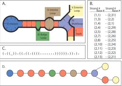
A system microstate can be stored in many different ways, as shown in Figure 6.1. Each

of these has different advantages: the flat (“dot-paren”) representation (Figure 6.1C) can

be used for both the input and output of non-pseudoknotted structures, but the

informa-tion contained in the representainforma-tion needs addiinforma-tional processing to be used in an energy

computation (we must break it into loops). Base pair list representation (Figure 6.1B)

allows the definition of secondary structures which include pseudoknots, but also requires

processing for energy computation. Loop representation (Figure 6.1D) allows the energy to

be computed and stored in local components, but requires processing to obtain the global

structure, used in input and output. While the loop graph cannot represent pseudoknotted

structures without introducing a loop type for pseudoknots (for which we may not know

(44)

primar-ily concerned with non-pseudoknotted structures this is only a minor point. In the future

when we have excellent pseudoknot energy models, we will have to revisit this choice and

hopefully find a good representation that still allows us similar computational efficiency.

We use the loop graph representation for each complex within a system microstate,

and organize those with a simple list. This gives us the advantage that the energy can be

computed for each individual node in the graph, and since each move only affects a small

portion of the graph (Figure 6.3), we will only have to compute the energy for the affected

nodes. While providing useful output of the current state then requires processing of the

graph, it turns out to be a constant time operation if we store a flat representation which

IV. Multiloop V. Exterior Loop I. Stack III. Bulge Loop II. Interior Loop VI. Hairpin

A.

B.

C.

D.

Strand # Strand #

Base # Base #

(1,1)

(1,3)

(1,4)

(2,4)

(2,5)

(2,7)

(2,8)

(2,10)

(2,11)

(2,12)

(2,13)

(2,31)

(2,2)

(2,1)

(2,29)

(2,28)

(2,26)

(2,25)

(2,24)

(2,23)

(2,22)

(2,21)

-(.((_)).((.((.((((...)))))).)).).

(45)

gets updated incrementally as each move is performed by the simulator.

We contrast this approach with that in the original Kinfold, which uses a flat

repre-sentation augmented by the base pairing list computed from it. Since we use a loop graph

augmented by a flat representation, our space requirements are clearly greater, but only in

a linear fashion: for each base pair in the list, we have exactly two loop nodes which must

include the same information and the sequence data in that region.

6.1.3 Reachable States: Moves

When dealing with a flat representation or base pair list for a current state, we can simply

store an available move as the indices of the bases involved in the move, as well as the rate at

which the transition should occur. This approach is very straightforward to implement (as

was done in the original Kinfold), and we can store all of the moves for the current state in

a single global structure such as a list. However, when our current state is represented as a

loop graph this simple representation can work, but does not contain enough information to

efficiently identify the loops affected by the move. Thus we elect to add enough complexity

to how we store the moves so that we can quickly identify the affected nodes in our loop

graph, which allows us to quickly identify the loops for which we need to recalculate the

available moves.

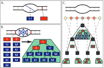
We let each move contain a reference to the loop(s) it affects (Figure 6.2A), as well as

an index to the bases within the loop, such that we can uniquely identify the structural

change that should be performed if this move is chosen. This reference allows us to quickly

find the affected loop(s) once a move is chosen. We then collect all the moves which affect a

particular loop and store them in a container associated with the loop (Figure 6.2B). This

allows us to quickly access all the moves associated with a loop whose structure is being

modified by the current move. We should note that since deletion moves by nature affect

the two loops adjacent to the base pair being deletion, they must necessarily show up in the

available moves for either loop. This is handled by including a copy of the deletion move in

each loop’s moves, and halving the rate at which each occurs.

Finally, since this method of move storage is not a global structure, we add a final layer

of complexity on top, so that we can easily access all the moves available from the current

state without needing to traverse the loop graph. This is as simple as storing each loop’s

(46)

complex’s available moves as shown in Figure 6.2C.

A.

B.

1, 1 1,1 1,2 1,3 2,1 2,2 2,3 3,1 3,2 3,3 1 2 1,1 1,2

1,3 2,1 2,2

2,3 3,1 3,2

3,3 2 1

C.

1,1 1,2 1,3 2,1 2,2

2,3 3,1 3,2 3,3 2

1

Figure 6.2: (A) Creation moves (blue line) and deletion moves (red highlight) are repre-sented here by rectangles. Either type of move is associated with a particular loop, and has indices to designate which bases within the loop are affected. (B) All possible moves which affect the interior loop in the center of the structure. These are then arranged into a tree (green area), which can be used to quickly choose a move. (C) Each loop in the loop graph then has a tree of moves that affect it, and we can arrange these into another tree (black boxes), each node of which is associated with a particular loop (dashed line) and thus a tree of moves (blue line). This resulting tree then contains all the moves available in the complex.

6.2