LONG-TERM RESPONSE TO SELECTION I. RELATION TO BREEDING POPULATION SIZE, INTENSITY, AND ACCURACY WITH ADDITIVE GENE ACTION

LONG-TERM RESPONSE T O SELECTION

I. RELATION T O BREEDING POPULATION SIZE, INTENSITY, AND ACCURACY WITH ADDITIVE GENE ACTION1

DEWEY L. HARRIS

Agricultural Research Service, U S . Department of Agriculture and Purdue University, West Lafayette, IN 47907

Manuscript received June 25, 1979 Revised copy accepted November 16, 1981

ABSTRACT

Dual CDC-6500 computers were used to simulate the probabilistic aspects of genetic selection and reproduction in random mating populations with additive gene action. These simulations involved either 10 or 20 replicates of 200 consecutive nonoverlapping generations for 72 combinations of breed- ing population sizes, mating ratios, selection intensities, and accuracies of

genetic determination of quantitative phenotypes. The results demonstrate that at least some long-term responses can be characterized by modified exponential functions that, with increasing generations, approach asymptoti- cally to limits whose expectations increase linearly with the inverse tangent of multiples of the expected initial responses. The multiplicative constants are greater for populations with large effective breeding population size than for those of smaller size. Agreement with and discrepancies from past theo- retical results are discussed. The supposition is made that the general form of these equations will be retained for broader situations than those simu- lated, but probably not for nonadditive gene action.

UMEROUS workers (GILL 1965a, b, c;

LATTER

1965a, b;

QURESHI

1968;

N

QURESHI, KEMPTHORNE and

HAZEL

1968) have used computer simula-

tion to study long-term genetic response to selection. This approach has been extremely informative about the nature of improvement from selection but has not yet led to mathematical formulae that allow the prediction of long- term response to selection. The capabilities of the Dual CDC-6500 computers at Purdue University made it feasible to study this problem with a greater volume of simulation. The primary purpose of this study was t o develop empirical formulae to describe long-term response to selection and to describe the relation of selection limits to factors affecting limits. A secondary purpose was to compare the results and the derived formulae to certain theoretical results from mathematical considerations. This comparison examined the valid- ity of the theoretical results since they are based upon assumptions that are not always justified.

The changes in a genetic population undergoing selection within the popu, 1 Journal Paper No. 7620, Purdue Agricultural Experiment Station. Joint contribution from USDA-ARS-NCR, IL-IN-OH Area and Department of Animal Sciences, Purdue University.

512 D. L. H A R R I S

lation for a quantitative trait have been of concern in numerous studies. Sev- eral studies have contributed to the development of the ability to predict short-term response to selection (DICKERSON and HAZEL, 1944; LUSH 1945 and earlier editions; COCHRAN, 1951 ; GRIFFING, 1960). The appropriate equa- tion for monoecious populations is:

AG

=

i

p G 1 (TG

AG =

%

{im

PGI+%

+

if

P G I ~

1

(TG

(1)

(2) and that for dioecious populations is

where AG is the single generation response to selection,

i

is the selection differential in standard deviation units, P G I is the correlation between I , the selection criterion,

G, the additive genetic value for the eslection trait or linear combination of traits (for single trait, mass selection, pcI will equal h, the square root of heritability for that trait),

( T ~ is the additive genetic standard deviation for the trait or combination of traits to be selected. The m or f subscripts indicate the male and fe- male subpopulations.

SMITH (1969), in a n approximate form, and ROBERTSON (1970b), developed the following formula (in ROBERTSON’S notation) for cumulative long-term response:

A G ( ~ ) = 2Nih { 1 - (1 - 1/2N)

‘30

where

i

is again the selection differential (each generation) in standard devia- tion units,

V , is the additive genetic variance (= v z G ) ,

(T is the phenotypic standard deviation,

N

is the breeding population size, and

AG(t) is the cumulative response from t generations of selection. Since

hz vA/u2,

AG(t)

=

2Nih ( 1

-

(1 - 1/2N)t} V , % _{( 3 )}

(4) and

=

2Ni V A / (T

=

2Nih

VA

M

ROBERTSON (1960) also obtained the latter result as an approximation to the expected limit when N i is small.

ROBERTSON (1960), following an earlier development by KIMURA (1957), noted the formula for the fixation probability, which for additive gene action would be

- z B i ( a / , ) p

1 - e

o e dx

o

B

-2N8x

dx

1 - e

-

1”

-23’’sc

-

-2.vi ( a / 6 )

U ( P >

=

LONG-TERM RESPONSE T O SELECTION 513

u ( p ) is the probability of fixation for that allele,

N

is the effective population size,

s =

i a / r

is the selective advantage of the homozygote of that allele, r is the phenotypic standard deviation,

a is the difference in the character selected between the homozygote for the specified allele and the homozygote for the contrasting allele, and

i is the selection intensity in standard deviation units, as above.

ROBERTSON deduced that because the square root of heritability ( h ) will re- flect the a l a values, selection limits should be a function of Nih. This formula is derived from monoecious population considerations; the extension for the case of dioecious populations with differing N ,

i,

and s or h for the two sexes is not completely apparent, although some conjectures may be made. This result is based on the assumption that ala-or equivalently s, and Ns, or

equivalently Nih-are small enough that second order terms are negligible. The SMITH-ROBERTSON formula (equations 3 and 4) involves a similar “weak selection” assumption that

V A

values change only due t o inbreeding and not because of any changes in gene frequencies resulting from the effectiveness of selection. The potential inadequacy of these formulae is emphasized by FRANK-

HAM’S (1977) results with the data of FRANKHAM, JONES and

BARKER

(1968)

and JONES, FRANKHAM and BARKER (1968) on selection for increased abdomi- nal bristle number in Drosophila melanogaster. FRANKHAM concluded that the responses to selection were not in particularly close agreement with those ex- pected from the SMITH-ROBERTSON theory.

MATERIALS A N D METHODS

Of the computer simulation studies cited above, the program used in the present study is most similar to that used by GILL (1965a, b, c) and QURESHI, KEMPTHORNE and HAZEL

(1968). The common characteristics of all populations simulated in the study being reported are:

1. Four pairs of chromosomes with ten equally spaced loci on each.

2. Recombination probability of 0.05 between adjacent loci, with independent (no crossover

3. Two alleles ( + and -) at each locus with an initial gene frequency of 0.25 for the

4. An initial conceptual infinite population with Hardy-Weinberg structure and no linkage

5. Genotypic values calculated as simply the number of

+

alleles in the genotype at all

6. Phenotypic values calculated as the genotypic values plus random normal deviates with

7. Three male and three female offspring (all full-sib t o each other) produced from each

8. Upper truncation mass selection of specified constant proportions within both sexes. 9. Random mating without replacement of a specified number of selected females to each selected male to give the specified number of matings (each male may be mated to more than one female, but each female is mated to only one male).

A fundamental difference from QURESHI, KEMPTHORNE and HAZEL (1968) and GILL (1965a, b, c) is our simulation of this structured random mating without replacement with a fixed interference) probabilities of recombination on different segments of a chromosome.

+

allele at all loci.

disequilibrium, with all generation 0 parents randomly drawn from this initial population.

40 loci (additive gene action with equal effects across all loci).

zero mean and appropriate variance to achieve the specified heritability.

514 D. L. HARRIS

number of offspring of each sex for each mating; they simulated a fixed number of random matings with replacement with each mating producing a single offspring of the specified sex. The consequences of this difference are not clear, but the former seems more representative of selection and mating in controlled breeding populations.

With the genotypic values calculated as specified above, there will be a minimum geno- typic value of 0 and maximum of 80, an initial population mean of 20, and an initial geno- typic variance of 15 in the simulated population. Thus, these means are the expected values for the generation 0 parents. When more individuals of one o r both sexes were selected than were needed for the matings, a random part of those selected was used in the simulated ma- tings. For dioecious populations, there may be different numbers of parents for the two sexes (N9,% and N f ) , different accuracies of selection (hnb and hr) and different selection intensities (i, and if). Thus, an early objective of this study was to ascertain the functions for dioecious populations analogous to the Nih deduced from equation (5) for monoecious populations. An- other purpose was to decide if that function would be fully appropriate f o r describing long- term response to selection or if some other function would be more appropriate because the assumptions behind equation (5) probably imply more loci than the 40 simulated.

Table 1 summarizes the 72 parameter combinations that were simulated with either 10 or 20 replicate 200 generation selections. These 72 combinations involve breeding population sizes ( N , = number of male parents per generation, N, = number of female parents), ac-

curacies of selection ( h , = heritability of simulated trait in male progeny and h, = herita- bility in female progeny) and intensities of selection ( P , = proportion of male progeny selected on phenotypic values for the simulated trait and Pj = proportion selected in females). The N , values representing effective population size and presented in Table 1 were calculated

2 2

1 1 1

N e 4 N , 4 N f

from the WRIGHT (1931) formula (- = -

+

-)

.

This formula is based on an assump-

tion of random mating with replacement of randomly selected males and females to produce a single random offspring for each mating. The assumption departs from the form of random

TABLE 1

Number of replicates for each combination of parameters

P,= 1/3 1 2 / 3 1/3 1

N,n Nf Ne h2 fra h; P , = 1/3 1/3 2/3 1 1

6 6 12 0.5

0.125 0.5 0.125

I2 12 24 0.5

0.125 0.5 0.125

4 I 2 12 0.5 0.125 0.5 0.125

6 18 18 0.5

L O N G - T E R M R E S P O N S E T O S E L E C T I O N 515

mating simulated. However, it was anticipated that the values calculated by this foimula would approximate the true values.

The parameter combination for paired matings ( N , = N f ) with P, = 1, Pf = '/3 were not included because of their expected equivalence to those for P, = 1/3, Pf = 1. Ten repli- cates were done for most parameter combinations. However, 20 replicates were simulated for the parameter combinations with non-zero expected selection response and with only six ma- ting pairs because of the expected greater variability of response. Thus, there are a total of 840 individual replicates.

The parameter combinations involve factors in which some levels are half of the other levels. This arrangement was made intentionally, so that for any of several potential dioecious formulae analogous to N i h , sets of equivalued expected limits among the 72 parameter com- binations would occur. Thus, those sets of parameter combinations whose replicated simula- tions yielded similar observed values for the limits provided clues as to the relevant formula.

R E S U L T S A N D DISCUSSION

Shape of long-term response

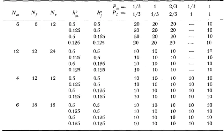
Four of the 72 parameter combinations are presented in Figures l a and lb. Presented here are CALCOMP plots of the generation genotypic means plotted against generation number. Figure l a shows five of the 10 replicates for

N,, =

Nf

= 12, P,n = P f

=

2 / 3 , and

=

= 0.125. The dots represent the

INITIRL POTENTIRL

70 .oO

10.00

I

I I I I I I I

125.0 160.0 175.0 2

GENE;PR~~PONS

,

.o 25.0 so .a 75 -0

15.w

12.91

-

_> 10.39:

0 c 0

z

7.75%

n

0

U

c 5.16;

Tr

I-

2 -58

.m

.O

FIGURE la.-Cumulative genetic response for N , = N f = 12, P, = Pf = -2/3, and h, = hf =

516 D. L. HARRIS

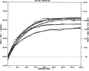
FIGURE 1b.-Cumulative genetic response with mean response and curve of average a, /3,

Upper left: 20 replicates for N, = N f = 6, P, = Pf = %, and h, = hf2 = 0.5

Upper right: 10 replicates for N, = N f = 12, P,, = Pf = %, and h, = hf2= 0.5

Lower left: First 10 replicates for N, = N f = 6, P, = Pf = %, and h, = h; = 0.125.

Lower right: First 5 replicates for N, = Nf = 12, P, = Pf = %, and h, = h; = 0.125. and '/ superimposed.

2

2

2

2

genotypic means for the individual generations. The stars represent the points at which complete fixation at all 40 loci occurred, plotted at the level of the genotypic mean at the generation in which fixation occurred. This mean

is usually described as the selection "limit." Genotypic means were constant after that, and the constancy of plots of simulated means is represented by the straight; lines. Superimposed upon these are five smooth curves, representing functioiis fitted to each of the five response curves. The curves are of the modi- fied ex1 onential form,

where g represents the generation number,

Po

= a -

Pr"

po represents the genotypic mean for generation g,

LONG-TERM RESPONSE T O SELECTION 51 7

RSMITZ (International Mathematical and Statistical Libraries, Inc. 1977).

This subroutine uses an approach suggested by GREGORY (1970) to iteratively and alternately fit a and /3 by ordinary Least Squares and fit y by iteratively finding the value that minimizes the error sums of squares with the Fibonacci technique. JAMES (1965) suggested the modified exponential curve as being an appropriate form for describing long-term response to selection.

The fitted modi€ied exponential curves in Figure l a do a reasonable job of characterizing each of the response curves, but the random nature of these re- sponses leads to slight departures from the smooth curve. Figure l b combines four sets of simulations, each involving a different parameter combination. The lower right section involves the same five replicates as Figure l a but with two curves superimposed, a smooth and a not-so-smooth curve. The not-so-smooth curve represents the generation means averaged across the five replicate simu- lations. The smooth curve represents the modified exponential curve obtained from the a,

p,

and y parameters estimated by the average of the five a,

p,

and

y values for each of the five smooth curves in Figure la. Similar smooth and not-so-smooth curves are superimposed on the other three sections of Figure lb. The four sections of Figure l b represent four quite different parameter com- binations as reflected in the shape of the response curves. The lower right curves involve parameters for larger populations, weaker selection and lower heritabilities ( N n a = N f

=

12, P, = Pf I

2/3,

hk

= h: = 0.125) which leads to relatively late fixation; the level of the average limit (genotypic means at fix- ation) is intermediate relative to the other parameter combinations simulated in this experiment. The lower left section of Figure Ib represents the first ten replicates for N ,

=

N f = 6, P,

=

Pf

=

2/3,

and h,

=

hf” = 0.125; that is, relatively small populations with relatively weak selection as a result of a large selection proportion and a low heritability. The limits achieved are relatively low and occur at intermediate numbers of generations in relation to other parameter combinations. In the upper left of this figure are 20 replicates of

N ,

=

N f = 6, P, = 35, and

gz

=

hf”

= 0.5 representing small populations with strong, effective selection that leads to relatively early selection limits of moderately high level but with considerable variability. In the upper right for

N ,

=

N f

=

12, P,

=

P f = Vi, and h: = hf”

=

0.5, large populations with strong, effective selection, a high relative level of the limits is seen. These limits were achieved in relatively few generations.

518 D. L. H A R R I S

when they change from slightly increasing curves to a flat straight line, a shape to which the modified exponential curve cannot conform. The second area of discrepancy is at generation 0, where the smooth curves are slightly below (less than) the known initial population mean of 20. This occurrence undoubt- edly results because, starting with gene frequencies of 0.25, the additive genetic variance increased in the early generations; thus, there was a tendency for some increase in the rate of response in the early generations before the rate began to decline. This increase followed by a decline gives a slight S-shape to the re- sponse curves. The modified exponential curve cannot conform to this S-shape but responds to it by giving fitted curves that extend below the initial mean at generation 0. Simulations for populations with initial gene frequencies less than 0.25 would show more of this S-shape and, therefore, more discrepancy. Similarly, simulated populations with initial gene frequencies greater than 0.25 would be likely to show less S-shape and less discrepancy. Thus, the discrep- ancy would be more trivial for simulated situations with initial gene frequen- cies higher than 0.25. Tables 2a-d present, along with other relevant statistics, the average estimated value for a,

p,

y for each of the 72 parameter combina- tions simulated along with their standard errors (se.).

Factors influencing limits and generations to limit

Tables 2a-d also present the mean limit across replicate simulations and the mean generations to limit across replicates, and their standard errors (s.e.)

.

Complete fixation is the point at which all loci become fixed (homozygous) for the same allele in all individuals. The four subsections of Table 2 correspond to each of the four population size parameter types. Within each subsection of the table, the parameter combinations are grouped according to the expected initial response, presented as calculated from equation (2). The

i

values are calculated as the expected selection differentials in standard deviation units, assuming selection of finite samples from a finite population with a normal distribution of the selection criterion. These values differ slightly from the expected values for the same selection proportions under truncation selection from an infinite normal distribution. The calculated values in Table 2 involve the “order statistics” considerations discussed by RAWLINGS ( 1976) and

HILL

(1976). The

i

parameters were calculated with the algorithm described by

HARTER

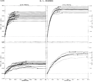
(1961) but with approximations of HASTINGS (1955) for the charac- teristics of the unit normal curve. Note that, for each population size type, those sets of treatment combinations with equal expected initial responses have similar observed limits and generations to limits.

These average limits and generations to limit are also presented in Figure 2.

L O N G - T E R M R E S P O N S E TO S E L E C T I O N 519

e x x + + + + a a Q Q Q o o o o

5 0 0 0 0 0 0 0 0 0 0 0 0 0 0 0

520 D. L. H A R R I S Y) is 2 -2

G *

5s

;

II

.??a S E 203

U I1

5

' S

2"

2 6

8 II

%

i z

3

$ s

o\

* -

e +

U

._ e

-

--r:

P 2 .c

*

2 3

a ?;* .S

c

6 :

b 2 .5

2 s

p1.Q

Y I U

-3

-

?.

5 s

h

w 2 %

E 2 .

E:

? E - 5

O Y _

t o

E E

0 " - .- n

3 1

u . r :

.-d

L r u

C? i

w

.- m E 8

,o L.

v 4-

3

.- $ e 0

s

E la M

-c .- B 2 e: U" s $ 0 E, .- a w e .- .- m

.r

z

U c. m x 4

z

a

LONG-TERM RESPONSE TO SELECTION 521

< N N x x x x x x t t III~IIIININ

----

N m m m c O C l m N N - N m ~ m mO m m h

H

8 8 8 8 8 8 8 8 8 8 8 8 Z 8 8 g g g 3 0 0 0 0 0 0 0 0 0 0 0 0 0 0 0 0 0 0 0 0

t I ti tI $1 tl $1 tl +I tl t l $1 t l $1 tl +I tl $1 ti tI t l

"1 e'4 c l ? ? T n q c ? 9 - '?a!-""! "!?,Ne N N M - W M - + M M _{w w m m a o o = m ~ m} tl tl $1 $1 tl ti t l t l tl ti t I t I $1 tl tI $1 tl $I tl tl

w...

10 W I D h h h h h h

m m m m m m o m m % $ Z : W 8 8 8 LO w w h h h h h h m m m m w m m

522 D. L. HARRIS Y 0 i- k -2

G g

2 I1

g m -3 e + a - -e

j g

2;

1

-

<

II

.U $ E

52

T;

3

.g

d

&

a g

3 " -

& $

w

'dr:

c

bnc

e

: s

Cl h u l

2 h

Y W

c ' .

5 2

q

-

9:

3 9

a h

-

k z

'2 U

G c1

$ ? 2 5 3% ? 2 E I 3 c? E s: n E

...

m U h

-

_",

4- ." E ...

-

3

U 3 e a bc 71 .- Eo 3 8 c, 'E 5 L k 0 ", n m

-

_.- + ... ... "

z

U a I $

z

x

s

Bo .m

70.00

6o.m

-

LD W z

'&! 5o.m

+

Q z

I-

U

4-

-

_{w .m}

C-.

30 .m

20 .m

10.00

LONG-TERM RESPONSE TO SELECTION

INITIAL POTENTIRL

I I I I I I I

126.0 160.0 176.0 D

GENEG~PONS

.O 25.0 so .o 76 .O

523

16.W

12.91

-

3. 10.23%

0 t- (13

2

7.76%

0

a

E

F

I-

6.16;;

2 .I

o .m

.O

FIGURE 2.-Mean across replicates of observed limits and generations to the limits for simulated traits of all parameter combinations grouped by effective breeding population size and expected initial response (see Table 2 for representation of parameter combinations by symbols).

ated with the greater initial response. For emphasis, freehand outlines of the visualized bands are superimposed on Table 2. Also, the parameter combina- tions for the intermediate effective population size of N e

=

18 are plotted with

a broader pen. The relationship between the arrangement within each band and the expected initial response can be noted by a detailed reference to the definition of the symbols in Tables 2a-d. Both

N e

and (

i m h

+

i f h f ) / 2 are rele- vant functions needed as elements of a more complex function to quantify, for dioecious populations, the influence of breeding population size, intensity of se- lection, and accuracy of selection upon the average limits and average genera- tions to limits.

Predicted limits

524 D. L. H A R R I S

The KIMURA-ROBERTSON formula for the limit (equation 5 ) and the SMITH-

ROBERTSON

formula (equation 4), extended to the limit, both indicate that the expected limits are “a function of Nih” for the single-trait monoecious situation.

N i h is proportional to N AG (see equation 1 )

.

This observation, combined with the observations in the previous section, raises the question of whether analo- gous dioecious predictions can be obtained by substituting N,(i,h, -k ifh,) / 2 ,

which is proportional to N e AG (equation 2), for Nih in these formulae. The results of this substitution in both formulae for predicted limits are also pre- sented i n Tables 2a-d. Study of these calculated values and comparison of them with the average observed limits for the simulated populations show good agreement only when the total response t o selection is small (limits less than 60) j that is, f o r weak selection or low N e or both, the SMITH-ROBERTSON and

KIMURA-ROBERTSON formulae agree with each other and are in reasonable agreement with the observed results. This agreement could have been expected from the assumptions involved in those formulae.

However, for stronger selection and/or larger population size, the SMITH- ROBERTSON results considerably overpredict observed responses. This discrep- ancy is especially obvious for those cases in which the SMITH-ROBERTSON predicted limit is considerably greater than the initial potential of 80, the max- imum value the simulated limits can possibly achieve. The inadequacy of the SMITH-ROBERTSON formula for these cases results from the number of loci and the magnitude of individual effects that were simulated in relation to the assumptions. The number of loci for which the SMITH-ROBERTSOX formula would seem to give a reasonable approximation is considerably greater than the simulated 40. This inadequacy may also explain why the FRANKHAM

(1977) results for abdominal bristles in Drosophila melanogaster are not in particularly good agreement with the SMITH-ROBERTSON formula. Presumably, the number of loci influencing abdominal bristle number is relatively small.

These results leave doubt as to the reliability of the SMITH-ROBERTSON for- mula and, thereby, to the development of JAMES (1972), in which that formula was used to obtain some elegant results concerning optimum selection schemes for maximizing long-term responses to selection.

LONG-TERM RESPONSE TO SELECTION 525

ences occur both in the assumption of small and constant (over time) selection advantage or disadvantage for each allele and in the assumption of indepen- dence between loci (resulting from free recombination between loci during crossingover). In addition, as noted earlier, the assumption behind WRIGHT’S

(1931) formula for effective population size,

N e ,

was not equivalent to the con- ditions simulated. Other works (LATTER, 1965b, 1966;

HILL

and ROBERTSON,

1966; ROBERTSON, 1970a) indicate that linkage reduces limits relative to free recombination. Since only one linkage arrangement-four chromosome pairs with ten equally-spaced loci with 0.05 probability of recombination between adjacent loci-was simulated, it is not possible, in this paper, to separate the effects of linkage being present from the effects of s or N i h not being small. Further studies are planned to see if departures from the KIMURA-ROBERTSON formula still occur when free recombination is simulated, to study the effects of varying chromosomal and linkage arrangements, and to develop more pertinent formulae for effective population size.

For the population size of N , =

4,

NI = 12, the KIMURA-ROBERTSON for- mula gives some predicted limits equivalent to those for populations with N ,

=

N f = 12, but at different expected initial responses. This equivalence is due to

equivalence of N e (i,h,

+

i&)

/ 2 terms. In these cases, the difference in values of Ne is exactly compensated for (in the predicted value but not in the observed simulation results) by the differences in

(i&,

+

i,h,)/2. The observed re-

sults for these predicted equal value situations show greater limits for the larger N e , small

(i,&

+

i f h f ) / 2 combinations than for small N e , large aver- age ih. These differences strongly suggest that the appropriate formula is not “a function of Nih” nor of its dioecious analogue, N,(i,h,

+

ifh,)/2. A more complex formula seems necessary to approximate the desired results adequately. The desire formula should involve N e and should involve (imhm

+

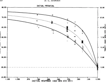
i,hf)/2 but should not simply involve their product.

Relation of limits to initial response and egective population size

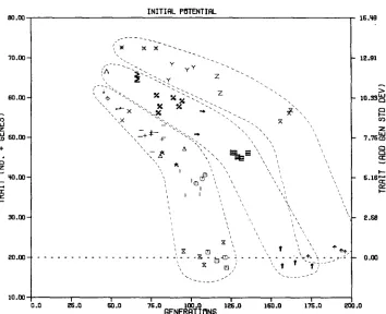
Figure 2 and Table 2 point to a strong relationship between the limits to selection and the initial response; it is informative to rearrange the points on Figure 2 by a plot of the limits versus the initial response as in Figure 3. The reversed abscissa scale in Figure 3 was made to emphasize the relationship to Figure 2. With this arrangement of the observations, we see, even more defi- nitely, three bands of points corresponding to the three effective populations sizes with a strong curvilinear relationship between the observed limit and the expected initial response. The departures from three smooth curves are the re- sult of the sampling variation generated by the random nature of the simulated genetic mechanism. All three of these bands coincide at the initial population mean of 20 for parameter combinations with zero expected initial response, all increase in a curvilinear manner, and all seem to asymptotically approach, at different rates, the potential of 80 as the expected initial responses increase. Because the observed results lend doubts as to accuracy of either the SMITH-

526

m.m

m .a

w.m

-

(0

W z

% m.m

+

0

5

a

F

w.m

I-

-

3o.m

m .m

1o.m

1

D. L. HARRIS

-

INITIAL PDTWTIRL

*\ -\

. . .

I I 1 I I I I I

6 1.W .m .ea, . l e 0

I N I T j x RESPdgE [ ROD%N STO%V I

16.W

12.91

-

> 10.39:

0

I-

(0

z i.m%

5 a a

I- 6 . 1 6 2

E

I-

2 . a

o.m

0

FIGURE 3.-Mean across replicates of observed limits for simulated trait for all parameter combinations plotted against expected initial response. See Table 2 for representation of param- eter combinations by symbols.

ing curves for describing the obvious relationships exhibited in these obser- vations became even more important. A variety of modified exponential functions with various transformations of the expected initial responses was evaluated, but these attempts did not yield curves that would closelj- fit the observed data.

LONG-TERM RESPONSE TO SELECTION 527

rated into the formulae by use of multiples of the expected initial responses with the constants of multiplication chosen to represent the specific effective population sizes ( N e ) simulated. Thus, the observed points could be reliably described with a series of three curves empirically found to be of the follow- ing form:

E ( a ) =/LO

+

K A V A , ( 7 )

where

2

K =

-

{TANw1 ( a w e

RI)}

$7-

with

E ( a )

=

expected limit

=

expected population mean as g

+

C O ,

po

=

initial population mean (generation 0),

RI = expected initial response to selection in additive genetic stan- dard deviation units

=

(pl - p0)/vd0

(im&

+

if

h f ) / 2

=

AG(''/CA

,

0

S w e

=

displacement factor for effective breeding population size N e ,

uA

=

additive genetic standard deviation for initial population, h = number of additive genetic standard deviations from initial

population mean (p,,) to maximum potential genotypic value (80

-

20)/d/15

=

15.49,

TAN-I ( ) symbolizes the inverse tangent or arctangent in radians of the quantity in parentheses; in other words, the number of radians in an angle that has the tangent given in parentheses, and

K

=

the expected fraction of the maximum potential change.

These three curves are presented in Figure 3 with estimated S N e values for

Ne

of 12, 18, and 24. Estimated S N e values were obtained for each of the parameter combinations by first equating equation (7) to the average ob- served limit and then solving for S N e Parameter combinations for each of the three sets of parameter combinations corresponding to the N e values of 12, 18, and 24 yielded quite similar estimates of S w e . But great differences in estimates occurred between these three sets. Thus, the different estimates within each set were averaged to give the three average estimates,

a,,

=

2.75,

SI,

=

4.18 and S,,

=

7.63.

Statistical Analyses

Since the form of the derived curves was hypothesized from observing the results, statistical tests of significance have restricted validity. Nevertheless, analyses were made to measure and indicate the goodness-of-fit, but they will be presented without the usual tests of significance.

528 D. L. HARRIS

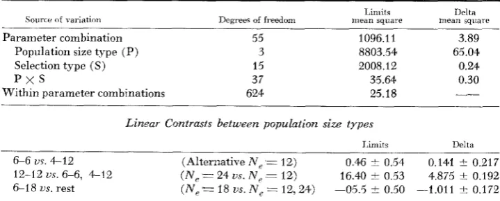
The analysis of variance in Table 3 results from a least squares analysis on the computer program of HARVEY (1977). Because of the unbalanced design, as is standard with the HARVEY program, the mean squares are calculated for each of the sources of variations, P, S, and P

x

S, adjusted for the other two. For the limits variable, breeding population size (P) and selection type (S) are seen to have large influences, with the interaction (P

x

S) having a negligible influence. Contrasts among the four population size types are presented along with their standard errors. The first of these contrasts points out the negligible difference in limits between the two different population size types with N e = 12. The second shows a tremendous difference between those small population size‘types

( N e

= 12) and the large type with N e

=

24. The third contrast shows that the observed limits for N e = 18 are almost exactly intermediate to those for N e

=

12 and those for N e = 24.

The observed limits were averaged for each parameter combination with non-zero expected initial response and estimates of

aNe

derived from these. The estimated

aye

were analyzed, and the resulting analysis of variance is pre- sented in the second part of Table 3, labeled “Delta.” Clearly, except for ran- dom variation, population size type is the only factor included in the design of this simulation experiment that has a n appreciable influence on the age or

Delta values.

sired number (10 or 20) for that parameter combination. For those simulations with non-zero expected initial response, the error standard deviations ranged from 0.507 to 1.180; most were less than 1.0 indicating very good fit. However, f o r cases in which the expected initial response (and thus

p )

was zero, the error standard deviations tended to be larger, with values from 0.727 to 1.632. However, the fitting of the modified exponential curve is rather meaningless for these cases. Thus, those simulations were excluded from the further analyses.

The linear contrasts among the four population size types for Delta pre-

TABLE 3

A n d y s e s of uariance for observed limits and corresponding Delta

(aATe)

ualues

Limits Delta Source of variation Dcgrees of freedom mean square mean square

Parameter combination 55

Population size type (P) 3

Selection type (S) 15

p x s

37

Within parameter combinations 624

1096.11 3.89

8803.54 65.04

2008.12 0.24

35.64 0.30

25.18

_-

Linzar Contrasts between populrrtion size types

J,imits Delta

LONG-TERM RESPONSE TO SELECTION 529

sented along with their standard errors indicate, as for limits, no appreciable difference between average estimated S N e for the two small population size types. The second contrast shows, as for limits, that most of the difference in

S x , is between the extreme population size types for N e

=

12 and N e

=

24. However, contrary to the result for limits, the third linear contrast shows that there is an appreciable amount of departure of the estimated Sx e from a linear

relationship with N e . If S x e of equation (7) was a linear function of N e , then E ( & ) would still be “a function of” N,R,

=

N i h as claimed by ROBERTSON

(1 960), even though the formula is not that of KIMURA (1957). However, this last contrast shows convincing evidence that a more complex relationship is involved. This analysis thus supports that the values of S N e for the parameter combinations for each of the N e of 12, 18, and 24 be averaged to give

SI,

=

2.75, S,, = 4.18, and

=

7.63, which are reflected in the curves plotted in Figure 3. It seems worth repeating that the

N e

values used here may only approximate the true values for the type of random mating.

Thus, both the empirically derived modified exponential curves (equation 6) for long-term response and the ARCTAN curve (equation 7) for expected lim- its, also empirically derived, are strongly supported by the observations gener- ating them. However, further simulations will be done for later papers to pro- vide independent observations for more reliable validation.

Curuature of long-term response

From studying equation (6),

pug = CY - PY”,

we see that po

=

a -

p,

and when y is a fraction, O<y<l, pg approaches

CY as g approaches infinity. In other words, a is the asymptote for pg as g in- creases and, thus, corresponds to the selection limit. Thus

p = a - p o

is the total response from p, to a, the limit. Note that

-

pn+2 - f&+1

pn+1 - pn

- Y

for all n

2

0. Thus, y is the fraction that the next change in generation means tends to be of the previous change. This fraction is constant throughout the curve, defines its curvature, and thus, will be termed the “decay of response.” Also,

P.+I

-

pn

= Y

P m - P n

530 D. L. HARRIS

may be found to lead to more complex functions with nonconstant “decay” and nonconstant “fractional responses”. As a special case of this last formula,

PI - Po

Ri

U A ~ -

- l - y =

P , -Po a - po

R I U A , , o r y r l -

a

-

p o

Thus, the three parameters, a,

p,

and y, i n equation (6) can be replaced by three alternative parameters, po, R, u ~and ~E ( a ) , ~ ,to describe expected long- term response to selection as

A simple form of this curve would be

E(ps) = Po

+

(1

-

ys} A U A o (9) where A uAo is the potential change,

K

and y

is the fraction of that change which is expected to be achieved, gives the curvature expected f o r the approach to the expected change.

Further Research

Several questions have been raised which cannot be answered with the body of simulation data presented in this paper. Further work is planned to develop formulae for effective breeding population size that are more precisely based upon the simulated situation than is the formulae of WRIGHT (1931) or

KIMURA and CROW (1963). None of these seem to accurately reflect the sim- ulated situation. Also, the effects of selection anticipated to reduce the effective population size as proposed by ROBERTSON (1961) need to be investigated. These considerations can be studied both by developing further mathematical theory and by adding calculations of effective population size to the simulation program.

L O N G - T E R M R E S P O N S E TO S E L E C T I O N 531

degree of dominance, the simple form of the modified exponential equation may not be realized for more complex gene action. In addition, the simulation situations of equal gene frequencies of 0.25 at all loci, equal allelic effects at all loci, and 40 loci on 4 chromosome pairs, etc., are also quite specific. HOW- ever, changes from these conditions do not seem likely (to the author, at least) to lead to departures from the general form of the modified exponential function. These variant conditions will likely influence the expected limit, which is the upper asymptote for the response curve.

Similarly, the arctan shape of the function for expected limits can also be expected to hold more generally but with differences from the simulated initial conditions reflected in the magnitude of the 6 parameters. Considerable addi- tional simulation study is anticipated to extend or modify these formulae.

With adequate generalization, a basis can be developed for improving the ability to predict long-term response to selection which is fundamental to the intelligent design of selection programs. Anticipated problems include the presumed difficulties in estimating population parameters such as h and 6 N e

Nevertheless, development of descriptive formulae is a necessary prerequisite

for developing prediction procedures.

The author wishes to acknowledge the valuable assistance of SCOTT NEWMAN in the execu- tion of many of the computer runs for this study and to express appreciation to him and to STEPHEN RICH and other Purdue University colleagues for valuable discussions during this study. Special appreciation is expressed to DR. RICH who suggested that the arctan function possibly has the appropriate shape.

L I T E R A T U R E C I T E D

COCHRAN, W. G., 1951 Improvement by means of selection. In: Proc. Second Berkeley S y m p . Math. Stat. and Prob. Edited by J. NEYMAN, pp. 449-470.

DICKERSON, G. E. and L. N. HAZEL, 1944 Effectiveness of selection of progeny performance as a supplement to earlier culling in livestock. J. Agr. Res. 69: 459-476.

FRANKHAM, R., 1977 Optimum selection intensities in artificial selection programmes: a n ex- perimental evaluation. Genet. Res. 30: 115-1 19.

FRANKHAM, R., L. P. JONES and J. S. F. BARKER, 1968 The effects of population size and selection intensity for a quantitative character in Drosophila. I. Short-term response to selection. Genet. Res. 12: 237-248.

Effects of finite size on selection advance in simulated genetic populations. Aust. J. Biol. Sci. 18: 599-617.

-

, 1965b A Monte Carlo evaluation of predicted selection response. Aust. J. Biol. Sci. 18: 999-1007.

-

, 1965c Selection and linkage in simulated genetic populations. Aust. J. Biol. Sci. 18: 1171-1187.

Design procedures and use of prior information in the estimation of parameters of the non-linear model v = a!

-

p Y X (unpublished Ph.D. thesis) North

Carolina State University, Raleigh, N.C.

Theoretical consequence of truncation selection based on the individual phenotype. Aust. J. Biol Sci. 13: 307-343.

GILL, J. L., 1965a

GREGORY, W. C., 1970

GRIFFING, B., 1960

IIARTER, H. L., 1961 HARVEY, R., 1977

5

32 D. L. H A R R I S

HASTINGS, C., JR., 1955 Princeton, N.J.

HILL, W. G., 1976

programmes. Biometrics 32 : 889-902. HILL, W. G. and A. ROBERTSON, 1966

Genet. Res. 8: 269-294.

erence Manual. IMSL, Houston.

1972

Approximation for Digital Computers. Princeton University Press,

Order statistics of correlated variables and implications in genetic selection

The effect of linkage on limits to artificial selection.

IMSL Library 3 Ref-

INTERNATIONAL MATHEMATICAL A N D STATISTICAL LIBI~ZRIES, INC., 1977

JAMES, J. W., 1965 Response curves in selection experiments. Heredity 20: 57-63. --,

Optimum selection intensity in breeding programmes. Anim. Prod. 14: 1-9. JONES, L. P., R. FRANKHAM and J. S. F. BARKER, 1968 The effects of population size and

selection intensity in selection for a quantitative character in Drosophila. 11. Long-term response to selection. Genet. Res. 12: 249-266.

Some problems of stochastic processes in genetics. Ann. Math. Stat. 28:

The measurement of effective population number. Evolu- tion 17: 279-288.

The response to artificial selection due to autosomal genes of large effect. I. Changes in gene frequency at an additive locus. Aust. J. Biol. Sci. 18: 585-598. ---, The response to artificial selection due to autosomal genes of large effect.

11. The effects of linkage on limits to selection in finite populations. Aust. J. Biol. Sci.

18: 1009-1023. -, 1966 The interaction between effective population size and link- age intensity under artificial selection. Genet. Res. 7: 313-323.

LUSH, J. L.. 1945 (and earlier editions) Animal Breeding Plans. Iowa State University Press, Ames, Iowa.

QURESHI, A. W., 1968 The role of finite population size and linkage in response to continued truncation selection. 11. Dominance and overdominance. Theor. Appl. Genet. 38: 264-270.

QURESHI, A. W., 0. KEMPTHORNE and L. N. HAZEL, 1968 The role of finite population size and linkage in response to continued truncation selection. I. Additive gene action. Theor. Appl. Genet. 38: 256-263.

variates. Biometrics 32 : 875-887. KIMURA, M., 1957

KIMURA, M. and J. F. CROW, 1963

LATTER, B. D. H., 1965a 883-901.

1965b

RAWLINGS, J. O., 1976

ROBERTSON, A., 1960

Order statistics for a special class of unequally correlated multinormal

A theory of limits in artificial selection. Proc. Royal Soc., B. 153:

234-249. __ , 1961 Inbreeding in artificial selection programmes. Genet. Res. 2:

189-194. -, 1970a A theory of limits in artificial selection with many linked loci. In: Mathematical Topics in Population Genetics. Edited b y K. KOJIMA. Springer-Verlag, New York. - , 1970b Some optimum problems in individual selection. Theor. Pop. Biol. 1: 120-127.

Optimum selection procedures in animal breeding. Anim. Prod. 11: 433442. SMITH, C.; 1969

WRIGHT, S., 1931 Evolution in Mendelian populations. Genetics 16: 97-159.