ABSTRACT
TOTH, ALEXANDER RAYMOND. A Theoretical Analysis of Anderson Acceleration and Its Application in Multiphysics Simulation for Light-Water Reactors. (Under the direction of Carl Kelley.)
In this work, we are concerned with both contributing to the theoretical foundation for Anderson acceleration, a method for accelerating the convergence rate of Picard iteration, and evaluating its performance in the context of coupled multiphysics problems in nuclear reactor simulation. Anderson acceleration proceeds by maintaining a depth of previous iterate informa-tion in order to compute a new iterate as a linear combinainforma-tion of previous evaluainforma-tions of the fixed-point map, where the linear combination coefficients are obtained by solving a linear least-squares problem. Prior to this work, theory for this method was fairly sparse, dealing mainly with showing its relation to quasi-Newton multisecant updating and, when applied to linear problems, GMRES iteration. The analysis presented in this work significantly expands upon the theory for this method. As this method is intended as an acceleration method for Picard itera-tion, our analysis concerns problems for which Picard iteration is convergent, namely when the fixed-point mapping is contractive. We present analysis which represent the first convergence results for limited-memory variations of Anderson acceleration and for nonlinear problems. Additionally, we present analysis for several variations on the standard Anderson acceleration method. In particular, we consider a variation which adjusts the memory utilization in order to maintain good conditioning of the least-squares problem, and we present local improvement results for the case in which the fixed-point map can only be evaluated approximately.
©Copyright 2016 by Alexander Raymond Toth
A Theoretical Analysis of Anderson Acceleration and Its Application in Multiphysics Simulation for Light-Water Reactors
by
Alexander Raymond Toth
A dissertation submitted to the Graduate Faculty of North Carolina State University
in partial fulfillment of the requirements for the Degree of
Doctor of Philosophy
Applied Mathematics
Raleigh, North Carolina 2016
APPROVED BY:
Pierre Gremaud Dmitriy Anistratov
Roger Pawlowski Carl Kelley
DEDICATION
BIOGRAPHY
ACKNOWLEDGEMENTS
I would like to thank my advisor, Dr. Tim Kelley, for providing me with this great opportunity and for all his help and guidance along the way. Next, I would like to thank my committee for helping me through this process. Finally, I would also like to thank all the math teachers I’ve had over the years for fostering my interest in mathematics at an early age, encouraging me to participate on the math team in high school, and challenging me and pushing my boundaries in this subject.
Next, I would like to thank all the folks with whom I regularly dealt and collaborated at Oak Ridge National Laboratory during my time spent there. In particular, thank you to Roger Pawlowski, Stuart Slattery, and Steven Hamilton for their research guidance and assistance in programming and computing matters, and thanks to Linda Weltman for her administrative support. And finally, thank you to all my office mates in the CASL intern office for making my working environment such an enjoyable one to be at, and for answering nuclear questions for the non-nuclear engineer in the room.
TABLE OF CONTENTS
List of Tables . . . .viii
List of Figures . . . ix
Chapter 1 Introduction to Coupled Multiphysics Problems . . . 1
1.1 Introduction . . . 1
1.1.1 Basic Definitions . . . 2
1.1.2 General Formulation . . . 3
1.2 Standard Solution Methods . . . 4
1.2.1 Picard Iteration . . . 4
1.2.2 Jacobian-Free Newton-Krylov . . . 7
1.2.3 Nonlinear Elimination . . . 9
Chapter 2 Tiamat Overview . . . 11
2.1 Introduction . . . 11
2.2 Participating Codes . . . 12
2.2.1 Bison . . . 13
2.2.2 COBRA-TF (CTF) . . . 14
2.2.3 MPACT . . . 16
2.2.4 Data Transfer Kit (DTK) . . . 18
2.2.5 PIKE . . . 19
2.3 Tiamat Simulation Process . . . 20
2.3.1 Fully-Coupled Problem Formulation . . . 21
2.3.2 Solution of Fully-Coupled Problem . . . 23
2.3.3 Performance of Picard Iteration . . . 26
Chapter 3 Analysis of Anderson Acceleration . . . 30
3.1 Review of Literature . . . 32
3.2 Standard Convergence Analysis . . . 35
3.2.1 Analysis for Linear Problems . . . 35
3.2.2 Analysis for Nonlinear Problems . . . 36
3.2.3 Numerical Tests . . . 41
3.3 Preconditioning . . . 43
3.4 Adjusting Storage Depth for Conditioning . . . 45
3.4.1 Numerical Tests . . . 53
3.5 Deterministic Errors in the Function Evaluation . . . 58
3.5.1 Linear Problems . . . 58
3.5.2 Nonlinear Problems . . . 62
3.6 Stochastic Errors in the Function Evaluation . . . 68
Chapter 4 Trilinos Anderson Acceleration Implementation . . . 70
4.1 Introduction . . . 70
4.2.1 Solver Options . . . 72
4.2.2 Step Implementation . . . 73
4.2.3 QR Management Routines . . . 74
4.2.4 Solver Creation . . . 82
4.3 Unit Tests . . . 83
4.3.1 Rosenbrock Test . . . 84
4.3.2 Chandrasekhar H-equation Test . . . 85
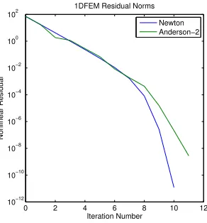
4.3.3 1DFEM Test . . . 87
Chapter 5 1D Coupled Model Problem . . . 89
5.1 Introduction . . . 89
5.2 Physical Models and Discretization . . . 91
5.3 Coupling Algorithms . . . 97
5.3.1 Picard Iteration . . . 97
5.3.2 Anderson Acceleration . . . 99
5.4 Numerical Results . . . 100
5.4.1 Picard Results . . . 101
5.4.2 Anderson Results . . . 104
Chapter 6 Anderson Acceleration for Tiamat . . . .107
6.1 Introduction . . . 107
6.2 Definition of Fixed-Point Maps . . . 107
6.2.1 Block Gauss-Seidel Map . . . 109
6.2.2 Block Jacobi Map . . . 110
6.2.3 Intermediate Map . . . 111
6.2.4 Scaling of Unknown Fields . . . 114
6.3 Implementation Details . . . 116
6.3.1 NOX Solver Creation . . . 116
6.3.2 Interfacing With PIKE . . . 117
6.3.3 Setting NOX Initial Iterate . . . 118
6.4 Numerical Results . . . 119
6.4.1 Single Fuel Rod Tests . . . 119
6.4.2 3x3 Mini-Assembly Tests . . . 144
6.4.3 17x17 Assembly Tests . . . 148
Chapter 7 Conclusion . . . .155
7.1 Anderson Acceleration Theory . . . 155
7.2 Coupled Multiphysics Problems . . . 158
References. . . .162
Appendices . . . .167
Appendix A Iterative Methods for Linear and Nonlinear Equations . . . 168
A.1 Linear Equations . . . 168
A.1.2 Stationary Iterative Methods . . . 170
A.1.3 Krylov Subspace Methods . . . 172
A.2 Nonlinear Equations . . . 174
A.2.1 Preliminaries . . . 175
A.2.2 Fixed-Point Iteration . . . 177
A.2.3 Newton’s Method . . . 178
A.2.4 Quasi-Newton Methods . . . 184
Appendix B Trilinos . . . 187
B.1 Trilinos Overview . . . 187
B.2 Relevant Packages . . . 187
B.2.1 Teuchos . . . 187
B.2.2 Epetra . . . 188
B.2.3 Tpetra . . . 188
B.2.4 Thyra . . . 189
B.2.5 Belos . . . 190
B.2.6 Anasazi . . . 190
B.2.7 Ifpack2 . . . 190
B.2.8 ML . . . 191
B.2.9 NOX . . . 191
B.2.10 PIKE . . . 191
B.3 Configuring and Building Trilinos . . . 192
Appendix C Tiamat Input Files . . . 194
C.1 17x17 Assembly Test Inputs . . . 195
C.2 Changes for 3x3 Mini-Assembly Tests . . . 201
LIST OF TABLES
Table 2.1 Comparison of block Gauss-Seidel vs block Jacobi for single rod Tiamat simulation at various power levels. Power damping factorω= 0.5 and max iteration count = 25 . . . 27 Table 2.2 Breakdown of solve and transfer timings (in seconds) for Tiamat HFP solve
phase at 75% power . . . 28
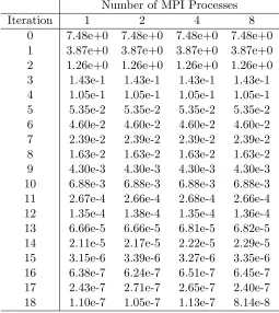
Table 3.1 H-equation iteration statistics for Newton-GMRES and fixed point iteration 42 Table 3.2 H-equation Anderson statistics, ω= 0.5 . . . 43 Table 3.3 H-equation Anderson statistics, ω= 0.99 . . . 43 Table 3.4 H -equation Anderson statistics,ω= 1.0 . . . 44 Table 4.1 Solving H-equation withω= 0.999 andN = 400 by Anderson-10, varying
the number of MPI processes utilized . . . 86
Table 5.1 1D model problem cross sections at various fuel temperatures with con-stant coolant temperature 565K . . . 94 Table 5.2 1D model problem cross sections at various fuel and coolant temperatures 94 Table 6.1 Comparison of Picard and Anderson-2 with each of the fixed-point maps
(Gauss-Seidel, intermediate, and Jacobi) for single-rod Tiamat simulation at various power levels. Damping factor = 0.5 and max iterations = 25 . . 120 Table 6.2 Comparison of Picard and Anderson-2 with each of the Gauss-Seidel and
Jacobi fixed-point maps for 3x3 Tiamat simulation at various power levels. Damping factor = 0.5 and max iteration count = 25 . . . 145 Table 6.3 Average application solve time(s) for Tiamat 3x3 tests at 100% power . . . 145 Table 6.4 Iterations to convergence for Tiamat 3x3 tests at various damping level,
100% power . . . 147 Table 6.5 17x17 assembly Tiamat test results, damping factor 0.5 . . . 149 Table 6.6 Average application solve time(s) for Tiamat single-assembly tests . . . 149 Table 6.7 Anderson-2 with Gauss-Seidel map with varying mixing parameter . . . . 152 Table 6.8 17x17 assembly Tiamat test results with 47-group cross section libraries
and damping factor 0.5 . . . 154 Table 6.9 Average application solve times for single-assembly Tiamat tests with
LIST OF FIGURES
Figure 2.1 Codes utilized in the Tiamat code coupling . . . 12
Figure 2.2 Bison 2-D axisymmetric finite element representation of a fuel rod; the radial dimension is scaled by a factor of 100 . . . 13
Figure 2.3 Subchannel representation utilized by CTF for a 3x3 array of fuel rods . . 15
Figure 2.4 Schematic of the MPACT solution process, coupling 2D/1D treatment of the transport equation with 3D CMFD acceleration (from [57]) . . . 18
Figure 2.5 Variation of the inlet coolant temperature (in blue) and power level (in red) during ramp of Bison from cold zero-power (CZP) to hot full-power (HFP) . . . 20
Figure 2.6 Data transfers utilized by Tiamat in the fully-coupled hot full-power (HFP) solve phase . . . 22
Figure 2.7 MPI communication layers in Tiamat . . . 26
Figure 2.8 Block Gauss-Seidel iterations to convergence for Tiamat single-rod simu-lation, varying the damping factor and power level . . . 29
Figure 3.1 Solving H-equation with Anderson-10 for various ω . . . 53
Figure 3.2 Solving H-equation by Algorithm 5 with m = 10 for various ω and con-dition number bound τ . . . 55
Figure 3.3 Solving H-equation with ω= 0.9999 and initial residual norm reduced by a factor δ from the base case . . . 56
Figure 3.4 Solving H-equation with ω = 0.99999 and initial residual norm reduced by a factor δ from the base case . . . 57
Figure 4.1 Convergence behavior and loss of orthogonality in the QR factorization of the least-squares coefficient matrix for H-equation test problem, m = 10, ω= 0.9999 . . . 80
Figure 4.2 Solving the Rosenbrock function by Anderson-2 . . . 85
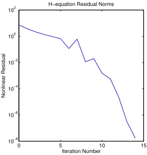
Figure 4.3 Solving H-equation with ω = 0.99 by Anderson-5 with acceleration de-layed until iteration 5 . . . 87
Figure 4.4 Solving the nonlinear heat conduction equation by Newton’s method and Anderson-2 . . . 88
Figure 5.1 Oscillatory temperature shift in Insilico/AMP coupling . . . 90
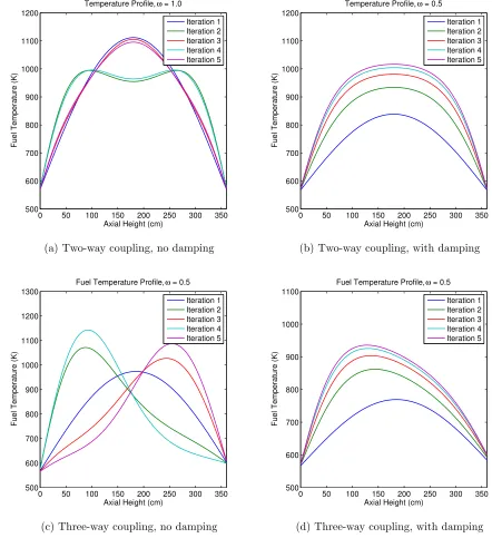
Figure 5.2 Fuel temperature behavior for the model problem, without and with damping . . . 102
Figure 5.3 Picard iterations to convergence, varying damping factor . . . 103
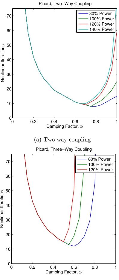
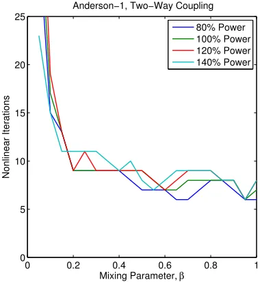
Figure 5.4 Nonlinear iterations to convergence for two-way coupling . . . 105
Figure 5.5 Nonlinear iterations to convergence for three-way coupling . . . 106
Figure 6.2 Anderson-2 iteration counts for single-rod Tiamat tests at several power levels, varying the damping factor . . . 123 Figure 6.3 Relative fixed-point residual histories from Tiamat single-rod tests at
100% power for Picard iteration and Anderson acceleration with various storage depth parameters . . . 124 Figure 6.4 Average fuel temperature computed by Picard iteration with Gauss-Seidel
map, and relative difference between this curve and Anderson solutions . 127 Figure 6.5 Average clad temperature computed by Picard iteration with
Gauss-Seidel map, and relative difference between this curve and Anderson so-lutions . . . 127 Figure 6.6 Average fission rate computed by Picard iteration with Gauss-Seidel map,
and relative difference between this curve and Anderson solutions . . . 128 Figure 6.7 Average heat flux computed by Picard iteration with Gauss-Seidel map,
and relative difference between this curve and Anderson solutions . . . 128 Figure 6.8 Varying CTF global energy balance tolerance in Tiamat single-rod tests . 132 Figure 6.9 Varying MPACT scalar flux tolerance in Tiamat single-rod tests . . . 133 Figure 6.10 Varying Bison JFNK tolerances in Tiamat single-rod tests . . . 135 Figure 6.11 Varying temperature scaling for Anderson-2 single-rod Tiamat tests with
the Gauss-Seidel map . . . 137 Figure 6.12 Varying temperature and density scaling for Anderson-2 single-rod
Tia-mat tests with the Jacobi map . . . 139 Figure 6.13 Varying power and heat flux scaling for Anderson-2 single-rod Tiamat
tests with the Jacobi map . . . 140 Figure 6.14 Comparison of Anderson-2 and JFNK with block Jacobi map for Tiamat
single-rod tests. JFNK uses a constant forcing term of 0.1 or 0.01, or an adjustable forcing term with initial value 0.1 . . . 141 Figure 6.15 Comparison of Anderson-2 and JFNK with block Gauss-Seidel map for
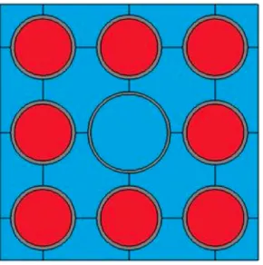
Tiamat single-rod tests. JFNK uses a constant forcing term of 0.01 . . . . 143 Figure 6.16 3x3 mini-assembly layout, with 8 UO2 fuel rods (in red) and a central
guide tube . . . 144 Figure 6.17 17x17 assembly lattice with 264 UO2 fuel rods (in blue), 24 guide tubes
(in white), and 1 instrument tube (in orange) . . . 148 Figure 6.18 Assembly averaged fuel temperature computed by Picard iteration with
Gauss-Seidel map, and relative difference between this curve and Ander-son solutions . . . 150 Figure 6.19 Assembly averaged clad temperature computed by Picard iteration with
Gauss-Seidel map, and relative difference between this curve and Ander-son solutions . . . 150 Figure 6.20 Assembly averaged fission rate computed by Picard iteration with
Gauss-Seidel map, and relative difference between this curve and Anderson so-lutions . . . 151 Figure 6.21 Assembly averaged heat flux computed by Picard iteration with
Chapter 1
Introduction to Coupled
Multiphysics Problems
1.1
Introduction
1.1.1 Basic Definitions
In this section, we introduce several important definitions for describing multiphysics coupling: • Coupled physics - When the solution of one set of physics depends on the solution of
another set of physics, theses physics are said to be coupled.
• Degree of physics coupling - The level of influence one set of physics has on another set. Two sets of physics are said to be strongly coupled if a change in the solution of one set results in a large change in the solution of the other. Otherwise, if a change in the solution of one set of physics results in a negligible change in the solution of the other, the sets of physics are said to be weakly coupled.
• Directional coupling - The manner in which two sets of physics depend on each other. Two sets of physics are said to be two-way coupled of the solution of each set is dependent on the solution of the other. Conversely, the sets of physics are said to feature one-way or forward coupling if the solution of only one set is dependent on the other. In this case, one set of physics may be solved independently of the other, possibly simplifying the solution of the coupled system.
• State variables - The set of variables that a single-physics application is solving for. • Residual (constraint) equation - The system of equations that a physics code solves to
compute the solution state variables. These are often generated from conservation or balance laws.
• Response function - A quantity of interest which a code is used to compute. This may cor-respond to the state variables themselves, but more generally may include postprocessed values computed from state variables and other independent parameters.
1.1.2 General Formulation
We now describe coupled multiphysics with mathematical rigor. We first consider a single-physics application. The residual equation corresponding to this application is given by
f( ˙x, x,{pl}, t) = 0, (1.1)
where
• x∈RNx is the vector of state variables,
• x˙ ∈RNx is the time derivative of the state variables,
• {pl}={p0, . . . , pNp−1}is the set of independent parameter sub-vectors,
• tis the time variable.
It is of interest to determine the state variables which solve this residual equation over some time interval of interest. In this work, we will be more concerned with solving steady state problems, for which (1.1) simplifies to
f(x,{pl}) = 0. (1.2)
This form may still be used to describe transient simulation, in which case this formulation represents the set of equations being solved for a given time step.
It is fairly straightforward to extend this formulation to coupled multiphysics problems. We now consider a set of Nf single-physics applications. Application i has its own residual
equation which it solves, as described by (1.2). Some of the set of parameter sub-vectors for this application may depend on state variables or other data from the other applications, so we partition the parameter sub-vectors into {zi,j}, the sub-vectors which depend on the solution
to other applications, and {pi,k}, the remaining sub-vectors whose values are independent of
the other applications. We then write the residual equation corresponding to application ias
fi(xi,{zi,j},{pi,k}) = 0, for i= 0, . . . , Nf −1. (1.3)
As the coupling parameters depend on some collection of state variables and independent pa-rameters from other applications, we can express them as follows
zi,j =ri,j({xm},{pm,n}). (1.4)
• {pm,n} = {p0,0, . . . , p0,Np0−1, . . . , pi,0, . . . , pi,Npi−1, . . .} is the set of all independent
pa-rameter sub-vectors for all applications,
• ri,j is a transfer function which maps state variable and parameter data from the other
applications to compute a dependent coupling parameter vector. This notation may bury significant complexity, as these transfer functions may involve computation of response functions, parallel communication, volume averaging, interpolation, etc. In practice, the dependencies of the transfer functions should be fairly sparse, usually mapping data from only a single application to a parameter vector for another.
Making the substitution (1.4), the above residual equation becomes
fi(xi,{ri,j({xm},{pm,n})},{pi,k}) = 0, for i= 0, . . . , Nf −1. (1.5)
Associated with this multiphysics system are the response functions
gi({xm},{rj,k({xm},{pm,n})},{pm,n}), for i= 0, . . . , Ng−1. (1.6)
The problem at hand is then to determine a collection of state variables {xm} such that
each residual equation (1.5) is simultaneously solved.
1.2
Standard Solution Methods
In this section, we overview standard solution methods which have frequently been used in solving coupled multiphysics problems. We note that the available solution methods may be limited by the capability of the physics codes being used. A code may have the capability to expose residual evaluations to the user, or it may only be able to solve for the state variables and return the solution or some post-processed response functions. Which data are exposed to the user will dictate which solution methods may be utilized.
1.2.1 Picard Iteration
The main advantage for this method is its simplicity of implementation and flexibility. This method requires the minimum that can be expected of a physics code: that it can accept coupling parameters as inputs and return response functions. The only data that needs to be exposed are whichever response functions are required to evaluate the transfer functions for each of the single-physics applications. The solution state variables for a given application might not even need to be accessible, so long as the required response functions are. Single-physics applications may be treated as black boxes with internal workings opaque to the user. Termination of this sort of iteration is then generally determined by small changes in various response functions (1.6) for the coupled system from iteration to iteration. Because of this method’s flexibility in regard to leveraging existing software and its relative simplicity of implementation it has been very widely used in solving coupled multiphysics problems. In particular, it has been the standard method utilized in the Consortium for Advanced Simulation of Light-Water Reactors (CASL). It is utilized in the VERA core simulator [40], the main product of CASL, as well as Tiamat [45], the coupling on which we focus later in this work.
In order to implement a Picard iteration in attempt to solve a coupled multiphysics problem, one needs to define some order in which to solve the single-physics applications. The two most common types of Picard iteration in this context (so named after their similarities to the corresponding stationary iterative methods for linear systems) are:
• Block Jacobi - Data transfers between all applications are carried out at the same time, and each set of physics is independently solved.
• Block Gauss-Seidel - Single-physics applications are sequentially solved with updated solutions transferred to the other applications as soon as they are obtained.
That is, in block Jacobi there are alternating phases of solving each of the single-physics appli-cations, and then computing updated coupling parameters. Conversely, for block Gauss-Seidel the applications are solved one at a time in a sequential order, passing data as it is obtained. These represent the only two types of orderings when the coupled system comprises of only two applications, but additional orderings are possible when coupling more applications. This will be examined further in Section 6.2.
As a more concrete example , we consider the following two-application multiphysics system
f0(x0, r0,0(x1)) = 0, (1.7)
f1(x1, r1,0(x0)) = 0. (1.8)
• Givenx00, x01. • Forn= 0,1, . . .
– Solve f0(xn0+1, r0,0(xn1)) = 0 forx
n+1 0 .
– Solve f1(xn1+1, r1,0(xn0)) = 0 forxn1+1.
Note that in this, each of the transfer functions ,r0,0andr1,0, is evaluated using the approximate solutions that are present at the beginning of the iteration. We similarly represent the block Gauss-Seidel iteration as follows:
• Givenx0 0, x01. • Forn= 0,1, . . .
– Solve f0(xn0+1, r0,0(xn1)) = 0 forxn0+1.
– Solve f1(xn1+1, r1,0(xn0+1)) = 0 forx
n+1 1 .
In this, xn0+1 is transferred to the other application as soon as it is obtained, andf1 is solved given this updated value. Assuming that xn0+1 is closer to the solution than xn0, the residual equation f1 given these updated values should be closer to the actual problem we are looking to solve, so this should result in an improved approximation to the solution.
In general, a block Gauss-Seidel scheme is expected to converge in fewer iteration than a block Jacobi scheme, as it keeps the applications more tightly coupled in a sense. Additionally, because a block Gauss-Seidel scheme keeps individual physics components more tightly coupled, it will likely converge for several problems where a block Jacobi scheme does not, particularly if the sets of physics are very tightly coupled. However, as each of the single-physics solves for block Jacobi is independent, it is possible to execute each solve simultaneously, whereas single-physics solves need to be executed serially for block Gauss-Seidel due to the sequential nature of the solves. In a parallel computing environment, this simultaneous solution of single-physics systems may result in significantly lower time per block Jacobi iteration than that for a block Gauss-Seidel iteration. However, significant reduction in per iteration run-time requires careful load balancing so that each of the single-physics solves takes roughly the same time.
1.2.2 Jacobian-Free Newton-Krylov
An alternative solution method to Picard iteration which has been employed in coupled mul-tiphysics problems is Jacobian-free Newton-Krylov (JFNK) [29, 31]. In contrast with Picard iteration, where the individual sets of physics are treated in a partitioned manner and solved indepently, JFNK achieves a tighter coupling by solving all the sets of physics simultaneously. Because of this more tightly coupled treatment, and several other advantages that Newton-like methods offer, JFNK has become widely utilized in solving coupled multiphysics problems. For instance, JFNK is a foundational tool for the MOOSE (Multiphysics Object Oriented Simula-tion Environment) framework [20]. In MOOSE, the Galerkin finite-element method is used for discretization and geometric representation [7] and JFNK is used to solve the resulting systems of equations. The Bison nuclear fuel performance code [23], which is utilized in the Tiamat coupling that we introduce in Chapter 2, is built on this framework.
A more formal description of Newton’s method, JFNK, and convergence theory for these methods, is given in Appendix A. As the name JFNK suggests, this method is derived from Newton’s method, which solves the equation F(u) = 0 by iterating
uk+1 =uk+dk, (1.9)
where the Newton direction, dk,solves the linear equation
F0(uk)dk =−F(uk). (1.10)
In the context of coupled multiphysics problems, the residual F in the above equation is a monolithic residual which is comprised of the residual equations for each of the single-physics systems
F({xm},{pm,n}) =
f0(x0,{r0,i({xm},{pm,n})},{p0,j})
f1(x1,{r1,i({xm},{pm,n})},{p1,j})
.. .
fNf−1(xNf−1,{rNf−1,i({xm},{pm,n})},{pNf−1,j})
= 0, (1.11)
corre-sponding to this residual has the form
F0({xm}) =
∂f0 ∂x0 ∂f0
∂x1 . . .
∂f0
∂xNf−1
∂f1
∂x0
∂f1
∂x1 . . .
∂f1
∂xNf−1
..
. ... ...
∂fNf−1
∂x0
∂fNf−1
∂x1 . . .
∂fNf−1
∂xNf−1 . (1.12)
In this, the off-diagonal blocks, ∂fi
∂xj fori6=j, will be zero if none of the transfer functions{ri,k}
corresponding to the single-physics residualidepends on xj, and generally non-zero otherwise.
There are several drawbacks to forming and storing the full Jacobian matrix. First, for even moderately large problems, forming the Jacobian may be prohibitively expensive, either with respect to computation or storage. If the entire set of state variables{xm}containsN variables,
the Jacobian has N2 entries, which may be too large to store. Even if there are several zero off-diagonal blocks, the amount of computation and storage required for the full Jacobian may be excessive. Second, it may not be possible to compute the Jacobian at all. Not only does it require differentiating each single-physics residual with respect to its own state variables, but the state variables for other applications for which it has a non-zero dependence as well. Even if a given physics code can compute a Jacobian for its residual equation with respect to its own state variables, the off-diagonal blocks may be difficult to obtain.
To avoid forming a Jacobian matrix, (1.10) may be solved in a matrix-free manner by uti-lizing a Krylov method. For this, one simply requires a method of computing the action of the Jacobian matrix on a given vector, F0(uk)v. As with forming the full Jacobian,
comput-ing a Jacobian-vector product analytically may be infeasible or impossible. As a result, some approximation to the Jacobian-vector product may be the only possible option in many cases. In JFNK, the Jacobian-vector product is approximated using a finite difference. This finite difference approximation is as follows
F0(uk)v =
F(uk+v)−F(uk)
, (1.13)
whereis a perturbation parameter. We see that each finite-difference approximation requires only the evaluation of the residual equation at a small perturbation to the current solutionuk.
The individual residual equations may need to be scaled if they deal with quantities of vastly different magnitude, otherwise selection of the perturbation factor in the forward-difference Jacobian-vector product may be problematic.
Returning to the example system in Equations (1.7)-(1.8), we seek a solutionu∗= x
∗
0 x∗1
to the monolithic system
F x0 x1
!
= f0(x0, r0,0(x1)) f1(x1, r1,0(x0))
!
= 0. (1.14)
In order to apply JFNK to solve this system, we simply require the ability to evaluate the perturbed residual about the current iterates xn
0 and xn1
F x
n
0 +v0 xn1 +v1
!
= f0(x
n
0 +v0, r0,0(xn1 +v1)) f1(xn1 +v1, r1,0(xn0 +v0))
!
= 0. (1.15)
JFNK is attractive for several reasons. First, Newton-like methods feature fast local conver-gence. Second, Newton-like methods feature several globalization methods, i.e. line searches [17] or trust-region methods [30]. As a result, even with a poor initial iterate, Newton’s method will converge to a solution or fail to do so in a predictable manner. Lastly, this method ensures consistency upon convergence. A Picard iteration generally terminates upon small change in response functions. However, small changes in response functions may not necessarily imply convergence of the state variables, so it is possible for a Picard iteration to declare convergence prematurely. However, because JFNK deals with the actual residuals for the application codes, on solution of the composite residual, the state variables for each physics application will also be converged.
However, JFNK comes with its own disadvantages. First, this method is more restrictive in implementation than Picard. Each of the codes needs to provide access to the state variables for which it is solving, and be able to return its residual. Many codes work as black boxes, in which inputs are specified, and output response functions are returned. The internal workings of the codes are not exposed to the user, so access to state variables or a residual may not be provided, or a residual might not be computed at all. Second, while the nonlinear iteration is generally expected to converge in few iterations, it may require many iterations in the linear solve phase, and as one residual evaluation is required per linear iteration, this may be prohibitively costly. In this case, it is necessary either to have a good preconditioner or in some way reduce the cost of residual evaluations in the linear iterations.
1.2.3 Nonlinear Elimination
(1.5) depends, and using this relation to eliminate that system from the coupled problem. In this way, a coupled problem can be reduced to solving for only a subset of the single-physics systems, and the solution to any eliminated system can be recovered from the solutions for those that are solved. This can provide flexibility if the systems that are eliminated are preventing from utilizing more advanced solution methods, e.g. enabling the use of Newton’s method by nonlinearly eliminating a single-physics system for which we can not access a residual or compute Jacobian information.
As an example, again consider the two-component coupled system given by Equations (1.7) and (1.8). The residual equation f1(x1, r1,0(x0)) = 0 implicitly defines x1 as a function of x0, so we denote the solution of this equation given anyx0 byx1(x0). We can then rewrite (1.7) as
f0(x0, r0,0(x1(x0))) = 0. (1.16)
Chapter 2
Tiamat Overview
2.1
Introduction
We now restrict our focus to the specific case of coupled multiphysics problems in the context of nuclear reactor simulation. The particular coupling on which we focus in this work is called Tiamat [45]. Tiamat is one of several code couplings being developed by the Consortium for Advanced Simulation of LWRs (CASL). Tiamat is intended as a tool for pellet-cladding inter-action (PCI) analysis. A nuclear fuel rod is comprised of a stack of UO2 fuel pellets enclosed in a Zircaloy tube, referred to as the cladding. Initially there is a gap between the fuel pellets and the cladding, and this closes during operation as a result of thermal expansion and fission product swelling in the fuel pellets, and inward displacement of the cladding due to external coolant pressure. PCI refers to cladding failure due to strains caused by contact between fuel pellets and the surrounding cladding during operation, resulting in release of radioactive fission products into the coolant. Such behavior usually occurs as a result of rapid changes in the local power distribution during power maneuvers. PCI is a problem of significant interest to the nuclear industry, as reactor operating restrictions established to mitigate this issue may result in reduced power generation [10]. It is then desirable to improve upon modeling and simulation techniques for this problem, as this could result in improvements in fuel design and quantification of safety margins.
Figure 2.1: Codes utilized in the Tiamat code coupling
several conditions within the reactor, specifically the rate of heat generation from fission in the fuel, which is the main thermal source in the fuel, and the clad surface temperature, which acts as a thermal boundary condition. This is accomplished in Tiamat by coupling Bison with other CASL single-physics codes to provide the necessary feedback, specifically the MPACT neutronics [14] and COBRA-TF thermal hydraulics [50] codes. Bison in turn provides feedback to the other single-physics codes, as the fuel temperatures affects the fission heat generation rate, and the heat flux from the fuel to the coolant affects several important coolant properties. We are concerned with finding a solution to this fully-coupled problem as efficiently as possible. In the remainder of this chapter, we will first overview the major codes participating in this coupling in Section 2.2. We will then describe precisely the problem at hand and how it has previously been solved by Picard iteration in Section 2.3, and lastly we will briefly present numerical results illustrating the behavior of Picard iteration for this problem in Section 2.3.3.
2.2
Participating Codes
Figure 2.2: Bison 2-D axisymmetric finite element representation of a fuel rod; the radial dimension is scaled by a factor of 100
2.2.1 Bison
As has been stated, the Bison fuel performance code [23] is being developed to provide single-rod, fuel performance modeling capability, which we utilize in Tiamat in order to calculate figures of merit which indicate the potential for PCI failures in PWRs. Bison is built upon Idaho National Laboratory’s MOOSE framework [20], so it uses the finite element method for geometric representation and JFNK to solve the resulting systems of partial differential equations. It includes 1D, 2D, and full 3D modeling capabilities. The fuel rod geometric repre-sentation utilized by Bison within Tiamat is a 2D R-Z axially-symmetric, smeared-pellet model. This is illustrated in Figure 2.2, where the red region is fuel and the blue region is cladding. The system of equations that Bison solves is as follows
ρCp
∂T
∂t +∇ ·(−k∇T)−q = 0, (2.1)
∇ ·σ+ρf = 0. (2.2)
These equations represent conservation of energy and momentum respectively. In Equation (2.1), T, ρ, Cp, k, andqare the temperature, density, specific heat, thermal conductivity, and
stress tensor, through a strain tensor. The material models are strongly influenced by the time history, so the Bison application is inherently a transient code. The state variables that Bison solves for are the temperature distribution and the displacement field. The coupling between the temperature solution and the mechanical solution is non-linear due to the complex depen-dency of the material properties on temperature, stress, and strain. In addition to the above, Bison accounts for changing chemical composition of the fuel and clad by the following equation representing species conservation
∂C
∂t +∇ ·J+λC−S= 0, (2.3)
where C, λ, S, andJare the concentration, decay constant, source, and mass flux respectively for a given chemical species. This affects material properties, and causes swelling in the pellets due to production of fission product.
A core-simulator is traditionally uses a quasi-static model, with a series of steady-state calculations [45], but since the material models within Bison are strongly dependent on the time history this code must be run transient. Then, when coupling Bison with the other application codes, we solve Bison one time step at a time, while the other codes are solved in steady-state mode. We represent the residual equation resulting from discretizing Equations (2.1) and (2.2) for a given time step as follows
fB(xB, Tc, q) = 0. (2.4)
In this, the vector of state variables xB is comprised of fuel temperature and displacement
unknowns. Note, we also identify the quantities Tc and q in this equation. These are coupling
parameter sub-vectors. That is, they are the zi,j vectors defined in Section 1.1.2. These are
quantities that depend on solutions to other application codes which affect the solution of (2.4). In this case, Tc is the cladding surface temperature and q is the fission heat generation rate.
The dependence of Equation (2.1) onq is obvious, andTcacts as the outer boundary condition
in this equation. In (2.4), we suppress the independent parameter sub-vector notation, {pi,k},
from Equation (1.3), which can include things like geometry specifications or other reactor conditions which are do not depend on the solution of any application codes. As Bison utilizes JFNK internally, it computes this residual directly, though access for the user is not easily provided.
2.2.2 COBRA-TF (CTF)
Figure 2.3: Subchannel representation utilized by CTF for a 3x3 array of fuel rods
the two-phase flow. The three fields considered are liquid film, liquid droplets and vapor. For each field, the equations and solved are as follows
∂
∂t(αkρk) +∇ ·(αkρk~vk) =Lk+M
T
k, (2.5)
∂
∂t(αkρk~vk) +∇ ·(αkρk~vk~v
∗
k) =αkρk~g−αk∇P +∇ ·[αk(τk+Tk)] +M~kL+M~kd+M~kT, (2.6)
∂
∂t(αkρkhk) +∇ ·(αkρkhk~vk) =−∇ ·[αk( ~
Qk+~qTk)] + Γkhk+qw,k000 +αk
∂P
∂t. (2.7) These equations represent conservation of mass, momentum, and energy respectively. In these equations, the subscriptkdenotes the field under consideration. Some important quantities to note in this equation are the void fractionαk, the densityρk, the velocity field~vk, the enthalpy
hk, the pressure P, and the volumetric wall heat transferqw,k000 . For discretization, CTF utilizes
a simplified subchannel form of these equations. A subchannel refers to the gap between a collection of rods as illustrated in Figure 2.3. CTF defines control volumes over axial sections of subchannels, and enforces Equations (2.5), (2.6), and (2.7) over these control volumes. The method used by CTF to solve these equations is called the Semi-Implicit Method for Pressure-Linked Equations [43]. CTF additionally includes several internal models useful for reactor analysis, such as spacer grid models and built-in material properties.
state convergence, which are as follows:
• The amount of energy stored in the fluid. • The amount of energy stored in the solids. • The amount of mass stored in the system. • Global energy balance.
• Global mass balance.
These quantities are defined precisely in [50]. CTF declares steady-state convergence upon sufficiently small changes in these quantities relative to the time step.
We represent the discretized residual of the steady-state form of Equations (2.5), (2.6), and (2.7) as
fC(xC, q00) = 0. (2.8)
In this, xC represents the discretized form of the velocity field, density, enthalpy, etc. The
coupling parameter vector q00 is the heat flux from the fuel to the coolant. As was previously stated, the CTF conservation equations are discretized by integrating over control volumes, and this converts the volumetric wall heat transfer q000w,k to the total wall heat transfer qw,k. This
value can also be computed by integrating the heat flux from the fuel q00 over the cladding surface area which bounds the control volume, so the heat flux represents a source in (2.7). We note here that while CTF is governed by Equation (2.8), it does not include the capability to evaluate this residual. It only has the capability to solve for its state variables and return various response functions.
2.2.3 MPACT
The reactor core simulator MPACT [14] has been developed collaboratively by researchers at the University of Michigan and Oak Ridge National Laboratory to provide an advanced pin-resolved transport capability within VERA. This code solves the neutron transport equation
Ω· ∇ψ(r,Ω, E) + Σt(r, E)ψ(r,Ω, E) =
Z ∞
0 dE0
Z
4π
dΩ0Σs(r,Ω·Ω0, E0 →E)ψ(r,Ω0, E0)
+χ(r, E) 4πkef f
Z ∞
0 dE0
Z
4π
dΩ0νΣf(r, E0)ψ(r,Ω0, E0). (2.9)
and Σf is the fission cross section. These quantities represent probability densities of a neutron
undergoing each given type of interaction. Lastly, kef f is called the dominant eigenvalue, and
this represents the average number of neutrons born per fission event that go on to undergo a fission event. In 3-dimensional space, ψ is a 6-dimensional function (3 space, 2 angle, and energy), so due to the high dimensionality, several simplifications are generally made when solving this problem. First, rather than solving for the directionally dependentψ, one typically solves for various angular moments of the angular flux. Second, energy dependence is generally treated through the multigroup approximation. In this, the energy variable is partitioned into energy groups given by the collection of intervals {[Eg, Eg−1]}Ng=1G, and (2.9) is integrated over each of these energy group. This results in the following
Ω· ∇ψg(r,Ω) + Σt,g(r)ψg(r,Ω) = NG
X
g0=1 Z
4π
dΩ0Σs,g0→g(r,Ω·Ω0)ψg0(r,Ω0)
+ χg(r) 4πkef f
NG
X
g0=1 Z
4π
dΩ0νΣf,g0(r)ψg0(r,Ω0), g= 1, . . . , NG, (2.10)
where
ψg(r,Ω) =
Z Eg−1
Eg
dE ψ(r,Ω, E), (2.11)
χg(r) =
Z Eg−1
Eg
dE χ(r, E), (2.12)
Σx,g=
REg−1
Eg dEΣx(r, E)φ(r, E)
REg−1
Eg dE φ(r, E)
. (2.13)
In (2.13), the subscript x represents any of the reaction types, and the weighting function φ, known as the scalar flux, is the zeroth angular moment of the angular flux. As the scalar flux is not known a priori, the group cross sections are typically computed using approximate weighting functions. Accurately solving this multigroup equation requires high-fidelity approximation of these group cross sections, and such approximation can be rather expensive.
Figure 2.4: Schematic of the MPACT solution process, coupling 2D/1D treatment of the trans-port equation with 3D CMFD acceleration (from [57])
the method of characteristics, and the 1D problem is solved by a lower order approximation. For computing multigroup cross sections, MPACT utilizes either the subgroup method [15] or the embedded self-shielding method [65]. CMFD accelerates this 2D/1D scheme by globally rebalancing the flux with a diffusion-like equation on a coarse mesh using coefficients computed from a fine mesh approximate solution. The coarse mesh equation is formulated in such a way that its solution is consistent with the fine mesh solution.
As with the first two applications, we represent the discretized form of Equation (2.10) in the following residual form
fM(xM, Tf, Tw, ρw) = 0. (2.14)
In this, the vector of state variablesxm consists of group scalar fluxes and the dominant
eigen-value. The dependencies Tf, Tw, and ρw represent the fuel temperature, coolant temperature,
and coolant density respectively. These affect the solution of (2.10) through the dependence of the multigroup cross sections on these material properties. Like CTF, MPACT does not feature the capability to evaluate this residual given some input set of state variablesxM.
2.2.4 Data Transfer Kit (DTK)
an intermediate decomposition of the source mesh/geometry is utilized in order to localize and load balance search operations.
In Tiamat, DTK was used for determining the parallel MPI communication mappings and for moving all data between codes. Issues such as unit conversions, as each application code uses different units, and differing coordinate systems are handled within these data transfer objects. We describe the DTK data transfer objects which are utilized in Tiamat in more detail when describing the formulation of the coupled problem in Section 2.3.1
2.2.5 PIKE
PIKE is a package of Trilinos [27] which provides interfaces and various utilities for black-box code coupling. This framework is leveraged heavily throughout Tiamat. One of the main features utilized is the PIKE solver class, which provides an interface for solving couplings be-tween black-box physics codes which interact through transfers of coupling parameter data, i.e. problems formulated as described in Section 1.1.2. Two implementations of PIKE solvers are provided in the package: a block Jacobi solver and a block Gauss-Seidel solver. These solvers are concrete implementations of the Picard iterations that were outlined in Section 1.2.1. These solvers work with abstract interfaces for model evaluator and data transfer objects which are also defined in PIKE. A PIKE model evaluator is wrapper class for single-physics application codes. The main functionality of this class is to solve the underlying application and return response functions. Additionally, it provides several other routines for step control for time-dependent application codes. Tiamat includes concrete model evaluator implementations for each of the three application codes. A PIKE data transfer is an abstraction of a transfer func-tion. The purpose of this class is to provide an interface for mapping data computed by one application code to input arrays for other codes. In Tiamat, DTK is the primary driver in the implementations of the PIKE data transfer objects.
Some other important pieces from this package that are utilized throughout Tiamat are as follows
• Status tests - Status tests are used to check for convergence or failure of an iteration. Some of the status tests included with PIKE check for successful local convergence of each participating physics application, small changes in response functions of interest, or exceeding a maximum number of iterations.
Figure 2.5: Variation of the inlet coolant temperature (in blue) and power level (in red) during ramp of Bison from cold zero-power (CZP) to hot full-power (HFP)
• Multiphysics distributor - The multiphysics distributor class provides several utilities for parallel task management. It can create and provide MPI sub-communicators for model evaluator and data transfers, and is useful for checking whether an application or transfer exists on a given MPI process. Additionally, the multiphysics distributor includes utilities for parallel output.
2.3
Tiamat Simulation Process
1. Estimate the conditions at HFP in stand-alone MPACT/CTF as described above.
2. Model the transition from CZP to HZP in Bison. In this step, Bison simulates over a period of 100 seconds with the inlet coolant temperature linearly varied from 293K to 565K.
3. Model the transition from HZP to HFP in Bison. In this step, Bison simulates over a period of 48 hours with clad surface temperatures linear varied from 565K to the estimated value from CTF in Step 1, and the power distribution linearly varied from zero to the estimated value from MPACT in Step 1.
4. Model the reactor state at HFP for one or more time step.
The first three steps in this process represent a fixed-cost for any given Tiamat simulation. The last step, in which we solve the fully-coupled system given by the three single-physics codes for one or more time step, is where we focus our attention, as this is where improvement can be made through advancement in techniques for solving tightly coupled multiphysics problems. We first describe more precisely the problem being solved in this step, and the methods which have been used to solve it prior to this work.
2.3.1 Fully-Coupled Problem Formulation
In the fully-coupled solve phase, we seek solutions to each of the single-physics applications such that each system is simultaneously solved. That is, we seek single-physics solutions , x∗B, x∗C, and x∗M, which solve the following monolithic residual equation
F
xB
xC
xM
=
fB(xB, Tc, q)
fC(xC, q00)
fM(xM, Tf, Tw, ρw)
= 0, (2.15)
wherefB, fC, andfM are the single-physics residual equations defined in Equations (2.4), (2.8),
and (2.14). As we had previously noted, the auxiliary conditions for each of the single-physics residual equations comes from quantities computed by other physical systems, so it remains to explicitly define these coupling parameter sub-vectors. We do this using the concept of transfer functions introduced in Section 1.1.2. In the fully coupled solve phase, five data transfer objects are utilized, and they are as follows
Figure 2.6: Data transfers utilized by Tiamat in the fully-coupled hot full-power (HFP) solve phase
of the temperature distribution. We denote this transfer function as
q00=rC,B(xB). (2.16)
• Bison to MPACT: The fuel temperature computed by Bison is transferred to MPACT. Denote this transfer function as
Tf =rM,B(xB). (2.17)
• CTF to Bison: The clad surface temperature computed by CTF is transferred to Bison. Denote this transfer function as
Tc=rB,C(xC). (2.18)
• CTF to MPACT: The coolant temperature and density computed by CTF is transferred to MPACT. Denote this transfer function as
Tw
ρw
!
=rM,C(xC) =
rM,C,T(xC)
rM,C,ρ(xC)
!
. (2.19)
• MPACT to Bison: The power distribution computed by MPACT is transferred to Bison. Denote this transfer function as
For each of these data transfers, the general process for evaluating the transfer function is to first compute the desired quantity on the set of source processes, and then perform a parallel communication to pass the data to the correct target processes. In general, this parallel trans-fer can involve interpolation or some more complex method of moving data between meshes. However, in Tiamat this is simplified by performing all transfers on a coupling mesh, which corresponds to the coarsest application axial mesh in the simulation. In this case, this is the axial mesh used by both CTF and MPACT. The coupling mesh consists of the volumes given by subdividing each fuel rod at a given set of axial bounds. Transfers between MPACT and CTF are volume-to-volume, so these simply consist of copying data to the correct volume. For transfers from Bison to the other application, a post-processor first averages the values defined on the Bison finite element mesh over the coupling mesh cells, and transfers these averages. Transfers to Bison are volume-to-point, and this is accomplished by simply assigning the value at a given finite element node the averaged value for whichever volume in the coupling mesh contains it.
Now given the notation in Equations (2.16)–(2.20), we can represent the fully-coupled sys-tem (2.15) in the following form
F
xB
xC
xM
=
fB(xB, rB,C(xC), rB,M(xM))
fC(xC, rC,B(xB))
fM(xM, rM,B(xB), rM,C,T(xC), rM,C,ρ(xC))
= 0. (2.21)
Then, at each time step in the fully-coupled HFP solve phase we seek solutionsx∗B, x∗C, andx∗M such that Equation (2.21) is satisfied.
2.3.2 Solution of Fully-Coupled Problem
Algorithm 1 Block Gauss-Seidel Nonlinear Solve for Tiamat
1: Givenx0B, x0C, and x0M.
2: fork= 0,1, . . .until converged do
3: Transfer Bison to MPACT, Tfk =rM,B(xkB).
4: Transfer CTF to MPACT, Twk=rM,C,T(xkC) and ρkw =rM,C,ρ(xkC).
5: Solve fM(xM, Tfk, Twk, ρkw) = 0 for xkM+1.
6: Transfer MPACT to Bison, qk+1 =rB,M(xkM+1).
7: Transfer CTF to Bison, Tck=rB,C(xkC).
8: Solve fB(xB, Tck, qk+1) = 0 forxkB+1.
9: Transfer Bison to CTF, qk00+1=rC,B(xkB+1).
10: Solve fC(xC, q00k+1) = 0 forxkC+1.
11: end for
Algorithm 2 Damped Block Gauss-Seidel Nonlinear Solve for Tiamat
1: Givenx0B, x0C, and x0M.
2: fork= 0,1, . . .until converged do
3: Transfer Bison to MPACT, Tfk =rM,B(xkB).
4: Transfer CTF to MPACT, Tk
w=rM,C,T(xkC) and ρkw =rM,C,ρ(xkC).
5: Solve fM(xM, Tfk, Twk, ρkw) = 0 for xkM+1.
6: Transfer MPACT to Bison, qk+1 =rB,M(xkM+1).
7: if k >0 then
8: Damp the transferred power, qk+1= (1−ω)qk+ωqk+1.
9: end if
10: Transfer CTF to Bison, Tk
c =rB,C(xkC).
11: Solve fB(xB, Tck, qk+1) = 0 forxkB+1.
12: Transfer Bison to CTF, qk00+1=rC,B(xkB+1).
13: Solve fC(xC, q00k+1) = 0 forxkC+1.
Algorithm 3 Damped Block Jacobi Nonlinear Solve for Tiamat
1: Givenx0B, x0C, and x0M.
2: fork= 0,1, . . .until converged do
3: Transfer Bison to MPACT, Tfk =rM,B(xkB).
4: Transfer CTF to MPACT, Twk=rM,C,T(xkC) and ρkw =rM,C,ρ(xkC).
5: Transfer MPACT to Bison, qk=rB,M(xkM).
6: if k >0 then
7: Damp the transferred power, qk= (1−ω)qk−1+ωqk.
8: end if
9: Transfer CTF to Bison, Tck=rB,C(xkC).
10: Transfer Bison to CTF, qk00=rC,B(xkB).
11: Solve fM(xM, Tfk, Twk, ρkw) = 0 for xkM+1.
12: Solve fB(xB, Tck, qk) = 0 for xkB+1.
13: Solve fC(xC, q00k) = 0 for xkC+1.
14: end for
At normal operating conditions, the procedure outlined in Algorithm 1 will fail to converge due to oscillation in the solution induced by certain error modes [24]. A standard method that has been utilized to remedy this issue is to introduce a numerical damping. Algorithm 2 shows the same block Gauss-Seidel solution process, now with a damping applied to the power update. In this, ω ∈ (0,1] is a damping factor. While these damping factors are chosen ad hoc, it has been observed that factors in the range 0.3-0.6 generally perform fairly well [24, 39, 66].
The process that the block Jacobi solver follows is shown in Algorithm 3. This algorithm alternates between phases of performing all data transfers and then solving all application codes. As with block Gauss-Seidel, a damping on the power update is included, and this is generally required in order to obtain convergence of the iteration. It is important to note that the solves in this case need not be performed in sequential order, and this allows block Jacobi to more effectively utilize parallelism. Figure 2.7 shows the parallel distribution utilized in Tiamat. Each of the application codes exists in its own process space, and due to this design choice each of the applications can perform a solve simultaneously. Conversely, for block Gauss-Seidel there is significantly more processor idle time, as all processes associated with a given application are idle while another application is solving. Hence, in an ideal scenario in which each application requires the same solve time, the time required per block Jacobi iteration would be roughly one third of the time per block Gauss-Seidel iteration.
Figure 2.7: MPI communication layers in Tiamat
functions between coupled iterations. PIKE status tests are used in order to determine the global convergence of the coupled system. In order for a simulation to declare successful global convergence, each of the application codes must have successfully converged locally, and the following conditions for must be satisfied
• Bison: the absolute change in the maximum fuel temperature from iteration to iteration must be less than some user-defined toleranceT.
• CTF: the absolute change in the maximum coolant temperature and maximum clad sur-face temperature from iteration to iteration must be less thanT.
• MPACT: the relative change (in thel2 norm) of the power distribution is less than some user-defined toleranceq between Picard iterations, and the absolute change inkef f must
be less than some tolerance k.
The iteration fails if it takes more than a prescribed maximum iteration count.
2.3.3 Performance of Picard Iteration
Table 2.1: Comparison of block Gauss-Seidel vs block Jacobi for single rod Tiamat simulation at various power levels. Power damping factorω= 0.5 and max iteration count = 25
Power Level Method Iterations Solve Time (s) kef f Tf,max
25% Gauss-Seidel 9 303 1.23708 483.55
Jacobi 14 392 1.23708 483.54
50% Gauss-Seidel 7 292 1.23105 694.09
Jacobi 15 407 1.23106 693.92
75% Gauss-Seidel 8 332 1.22493 931.20
Jacobi 18 462 1.22497 930.18
100% Gauss-Seidel 8 353 1.21857 1194.67
Jacobi DNC
125% Gauss-Seidel 12 445 1.21214 1505.16
Jacobi DNC
First, in Table 2.1 are results from Tiamat simulations utilizing both block Gauss-Seidel and block Jacobi as the solution method at several power levels. The power levels are listed as a percentage of the rated power specified in the input. This determines the magnitude of the power compute by MPACT, which is then passed to Bison. The power appears linearly as a source in Bison’s residual equation (2.4), so the power level affects the strength of the coupling between the applications. Increasing the power increases the strength of the coupling, and thus the difficulty of the problem. We see that with the exception of 125% power, each block Gauss-Seidel iteration converges with comparable iteration counts and run times. At 125% power there is a significant increase in these quantities. For block Jacobi, there is a more obvious upward trend throughout. Performance is comparable at the two lowest power levels, but as it is increased further the iteration counts rise sharply, and it begins to fail to converge. These results indicate that for both methods the performance may suffer as the strength of coupling between the sets of physics becomes greater.
The dominant eigenvaluekef f and the maximum fuel temperatureTf,max are listed in this
table to indicate the level of agreement between these two solution methods. We see that the two methods agree well for the cases where they both converge.
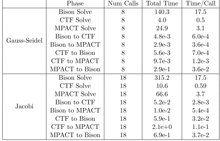
Table 2.2: Breakdown of solve and transfer timings (in seconds) for Tiamat HFP solve phase at 75% power
Phase Num Calls Total Time Time/Call
Gauss-Seidel
Bison Solve 8 140.3 17.5
CTF Solve 8 4.0 0.5
MPACT Solve 8 24.9 3.1
Bison to CTF 8 4.8e-3 6.0e-4
Bison to MPACT 8 2.9e-3 3.6e-4
CTF to Bison 8 5.6e-3 7.0e-4
CTF to MPACT 8 9.7e-3 1.2e-3
MPACT to Bison 8 2.9e-1 3.6e-2
Jacobi
Bison Solve 18 315.2 17.5
CTF Solve 18 10.6 0.59
MPACT Solve 18 66.6 3.7
Bison to CTF 18 5.2e-2 2.8e-3
Bison to MPACT 18 1.0e-2 5.4e-4
CTF to Bison 18 5.9e-1 3.2e-2
CTF to MPACT 18 2.1e+0 1.1e-1
MPACT to Bison 18 6.9e-1 3.7e-2
Gauss-Seidel. Because of this poor balance, little reduction in per iteration run-time results from simultaneously solving the applications in block Jacobi. It may be possible to bring Bison and MPACT into better balance with a different processor allocation. However, currently CTF is only parallelized to run with one processor per fuel assembly, and this may make good balancing of all three application codes problematic.
Next, Figure 2.8 shows the dependence of the performance of block Gauss-Seidel on the damping factorω. We note that block Jacobi behaves similarly. We observe that the performance of the method is very strongly dependent on this parameter. Fairly consistent performance is achieved over damping factors in range 0.4—0.6, and iteration counts rise rapidly away from this range. We also note that the performance depends noticeably on the power level. The left side of the curves remain static but on the right there is an upward trend. As a result, a damping factor that was suitable for a lower power level may be quite bad at higher powers. Additionally, the damping factor at which the method performs optimally is dependent on the power level. The optimum level shifts to the left as the power increased, and hence it difficult to say prior to simulation that one has chosen the best damping level for a given problem.
0.2 0.4 0.6 0.8 1 0
2 4 6 8 10 12 14 16 18 20
Damping factor
Iterations
80% Power 100% Power 120% Power
Figure 2.8: Block Gauss-Seidel iterations to convergence for Tiamat single-rod simulation, varying the damping factor and power level
Chapter 3
Analysis of Anderson Acceleration
In this chapter, we consider the algorithm proposed by Anderson in [2] which has come to be known as Anderson acceleration or mixing. The algorithm has also essentially been rediscovered and discussed under various names including Pulay mixing or Direct Inversion in the Iterative Subspace (DIIS) in [47, 48] for electronic structures calculations, Nonlinear Krylov Acceleration in [9], and IQL-ILS [16] for fluid-structure interaction calculations. Anderson originally consid-ered the algorithm in the context of solving a particular class of nonlinear integral equations, but it has subsequently gained popularity as a method to accelerate the convergence rates of Picard iterations. Given some mapping G:RN →RN, the method to solveG(u) =uproceeds as shown in Algorithm 4. In this, m is an algorithmic parameter that dictates the maximum depth for which previous iterate information is stored. We refer to the algorithm for any partic-ular value ofmas Anderson-m. Anderson-0 corresponds to standard Picard iteration. We need to store both u and one ofF(u) orG(u) at each iterate, so the storage burden is a maximum of 2(m+ 1) vectors. The additional cost in implementing this method as opposed to Picard iteration is dominated by the solution of the minimization problem. In the constrained form in Algorithm 4, the problem may be solved with a linear program or Lagrange multipliers. There are several equivalent ways to describe the algorithm with the minimization problem given in unconstrained form. If the minimization problem is solved in the l2 norm, as is standard, we then need only solve a linear least-squares problem. In the form originally posed by Anderson, we determine (θ(1k), . . . , θ(mkk)) which solve the problem
min (θ1,...,θmk)
F(uk) + mk
X
i=1
θ(ik)(F(uk−i)−F(uk))
, (3.3)
and then calculate
uk+1=G(uk) + mk
X
i=1
Algorithm 4 Anderson acceleration with inexact function evaluations
1: Given initial iterateu0 and storage depth parameterm∈N.
2: Setu1 =G(u0).
3: Set ˆF0=G(u0)−u0.
4: fork = 1,2,. . . do
5: Set mk= min{m, k}.
6: Set Fk=G(uk)−uk.
7: Determine α(k)= (α(k) 0 , . . . , α
(k)
mk) which solves
min
α=(α0,...αmk)T
mk
X
i=0
αiFk−mk+i
, (3.1)
subject to the constraintPmk
i=0αi = 1.
8: Set
uk+1 =
mk
X
i=0
α(ik)G(uk−mk+i). (3.2)
9: end for
Here the coefficients{αi(k)}and{θi(k)}are related byα(ik)=θ(mk)
k−ifor 0≤i < mkandα
(k)
mk =
1−Pmk
i=1θ (k)
i . Note that this requires the computation of the entire least-squares coefficient
matrix at each iteration. A third form which may be implemented more efficiently expresses the algorithm in terms of differences between successive iterates. For this, we determineγ(k)= (γ1(k), . . . , γm(kk))
T which solve the problem
min
γ kF(uk)− Fkγk, (3.5)
whereFk= (∆Fk−mk+1, . . . ,∆Fk) and ∆Fi =F(ui)−F(ui−1). Then, we calculate
uk+1=uk+F(uk)−(Uk+Fk)γ(k), (3.6)
whereUk= (∆uk−mk+1, . . . ,∆uk) and ∆ui=ui−ui−1. In this form{α
(k)
i }and{γ
(k)
i }are related
by α0 =γ0, αi = γi−γi−1 for 1≤ i≤mk−1, and αmk = 1−γmk−1. To update Fk and Uk
between iterations we append the new difference vectors at the end and drop the first columns if the storage limit has been reached. Solving the least-squares problem by taking QR factorization ofFk each iteration then results in a marginal cost ofO(m2kN) over Picard iteration. However, as mentioned in [62], we can obtain the QR factorization of Fk from that of Fk−1 , and this reduces the cost of the factorization toO(mnN) operations. We describe the method by which
substantial, especially if the evaluation of G is relatively expensive. However, there may be an appreciable difference in storage for problems of interest. Storing Fk and computing a QR
factorization each iteration requires at least temporary storage of both Fk and the Q factor, both of which have the same size. Conversely, when updating the QR factorization directly, only the Q and R factors need to be stored, and for reasonably sized storage parameterm, the storage burden of the R factor is negligible. Hence, for problems where N is very large, this yields an appreciable difference.
3.1
Review of Literature
We begin with an overview of previous work related to Anderson acceleration. Anderson ac-celeration is one of several methods which has been proposed and studied for the purpose of accelerating the rate of convergence for slowly converging series. Many acceleration methods are sequence transformations, i.e. methods which utilize the iterates produced by a slowly converg-ing sequence {xk} in order to construct a new, faster converging sequence {yk}. This includes
scalar acceleration methods such as Richardson extrapolation, the Aitken delta–squared pro-cess, and the Wynn epsilon method [8]. These methods can be applied to vector sequences in a component-wise manner, or one may utilize a vector extrapolation method such as reduced rank extrapolation, mimimal polynomial extrapolation, or modified minimal polynomial ex-trapolation [52]. Anderson acceleration differs from these methods in that it does not construct the original fixed-point iteration sequence. The acceleration from this method is derived from storing a history of previous iterates in order to compute a better approximation to the solution than the fixed-point iteration.
Again, Anderson acceleration was first proposed by Anderson in [2]. While he provides no rigorous analysis of the method, Anderson discusses several practical considerations. For instance, he claims that in practice, the method seems to perform best for small values of m, generally less than 10. Additionally, he describes how incorporate a mixing parameter into the algorithm. For this, the only difference in the above algorithm is that we replace (3.2) with
uk+1= (1−βk) mk
X
i=0
αiuk−mk+i+βk
mk
X
i=0
αiG(uk−mk+i), (3.7)
where the sequence of scalars{βk} are referred to as mixing parameters. This corresponds to a
damping factor in the context of Picard iteration. The choice of an appropriate mixing parameter is often necessary for the iterates to converge or obtain an acceptable rate of convergence.
may be viewed as a sort of quasi-Newton method. It is worth noting that the authors consider Anderson acceleration to solve F(u) = 0, not specifically as a fixed-point solver. To see this equivalence, consider (3.6). We rewrite this, now including mixing parameters, as:
uk+1=uk+βkF(uk)−(Uk+βkFk)γ(k). (3.8)
Then, assuming Fk is full rank, γ(k) is obtained by solving the normal equations, which gives
γ(k)= (FT
kFk)−1FkTF(uk). Substituting this into (3.8), we obtain
uk+1=uk−GkF(uk), (3.9)
where we have defined
Gk ≡ −βkI+ (Uk+βkFk)(FkTFk)−1FkT. (3.10)
In [19], it is claimed that this matrix Gk forms an approximate inverse Jacobian of F(x) in
the sense that the matrix minimizes kGk+βkIkF over all matrices which satisfy the inverse
multisecant condition
GkFk=Uk. (3.11)
This is referred to this as the Type-II method in [19]. Along these lines, they define the Ander-son’s family of methods according to
uk+1 =uk+βkF(uk)−(Uk+βkFk)VkTF(uk), (3.12)
whereVk∈Rn×msatisfiesVkTFk =I. The choiceVkT = (FkTFk)−1FkT gives the Type-II method
above. Conversely,VT
k = (UkTFk)−1UkT, under the assumption that UkTFk is nonsingular, gives
what is referred to in [19] as the Type-I method. For this choice of VkT we have
Gk≡ −βkI+ (Uk+βkFk)(UkTFk)−1UkT. (3.13)
As in [62], from the Sherman-Morrison-Woodbury formula this corresponds to the approximate Jacobian
Jk=G−k1 =−
1 βk
I+ 1 βk
(Uk+βkFk)(UkTUk)−1UkT, (3.14)
which satisfies the direct multisecant condition JkUk = Fk. According to [19] this minimizes
kJk+β1kIkf among matrices satisfying the direct multisecant condition.
In [62], it is shown that when Gis linear, i.e. G(u) =Au+bwith A∈RN×N and b∈