Improved Combinatorial Algorithms for the Inhomogeneous Short
Integer Solution Problem
Shi Bai1, Steven D. Galbraith1, Liangze Li2, and Daniel Sheffield1
1
Department of Mathematics, University of Auckland, Auckland, New Zealand.
2
School of Mathematical Sciences, Peking University, Beijing, China.
Abstract. The paper is about algorithms for the inhomogeneous short integer solution problem: Given (A,s) to find a short vectorxsuch thatAx≡s (modq). We consider algorithms for this problem due to Camion and Patarin; Wagner; Schroeppel and Shamir; Minder and Sinclair; Howgrave-Graham and Joux (HGJ); Becker, Coron and Joux (BCJ). Our main results include: Applying the Hermite normal form (HNF) to get faster algorithms; A heuristic analysis of the HGJ and BCJ algorithms in the case of density greater than one; An improved cryptanalysis of the SWIFFT hash function; A new method that exploits symmetries to speed up algorithms for Ring-ISIS.
Keywords:Short integer solution problem (SIS), SWIFFT hash function, subset-sum, knapsacks.
1
Introduction
The subset-sum problem (also called the knapsack problem) is: Given positive integers a1, . . . , am and an integers, to compute a vectorx= (x1, . . . , xm)∈ {0,1}mif it exists, such that
s= m
X
i=1
aixi.
It is often convenient to writea= (a1, . . . , am) as a row and x= (x1, . . . , xm)T as a column so thats=ax. The modular subset-sum problem is similar: Given a modulus q, integer vector a and integer s to find
x∈ {0,1}m, if it exists, such thats
≡ax (mod q).
The vector version of this problem is called the inhomogeneous short integer solution problem (ISIS): Given a modulus q, a small setB ⊆Zthat contains 0 (e.g., B ={0,1}or {−1,0,1}), ann×m matrixA (where typicallymis much bigger thann), and a column vectors∈Znq to find a column vectorx∈ Bm(if it exists) such that
s≡Ax (modq). (1)
If we want to be more precise we call this the (m, n, q,B)-ISIS problem. The original short integer solution problem (SIS) is the cases= 0, in which case it is required to find a solutionx∈ Bm such thatx
6
=0. Our algorithms solve both problems.
We unify the subset-sum and ISIS problems as the (G, m,B)-ISIS problem whereGis an abelian group (written additively),man integer andBa small subset ofZthat contains 0. The three motivating examples for the group areG=Z,G=Zq andG=Znq. An instance of the problem is a pair (A,s) withA∈Gmand
s∈G, and a solution is any vectorx∈ Bm(if one exists) such thats=Ax.
We now define thedensityof an ISIS instance, generalising a standard concept in the subset-sum problem. Recall that for integer subset-sum the density is defined to be m/log2(max{ai}).
Definition 1. Let Gbe a finite group. The densityof a (G, m,B)-ISIS instance isδ=(##BG)m.
If δ≤1 thenδ is the probability, over uniformly chosen elements (A,s) inGm
×G, that there exists a solutionx∈ Bmsuch thats=Ax. Ifδ
≥1 thenδis the average size of the solution set{x∈ Bm:s=Ax
}, over uniformly chosen elements (A,s) inGm
problem has low density. Ifδ ≈1 then we say we are in the “density 1” case. If δ≫1 then we are in the high density case. This informal notion is broadly consistent with the standard notion of density for the subset-sum problem overZwhenB={0,1}in the following sense: If one chooses the integersai uniformly in an interval {0,1, . . . , B} ⊂Z then max{ai} ≈B, and the density is approximatelym/log2(B). Taking
G=ZB, our definition gives density 2m/B. One sees that the notion of “low density” with both definitions corresponds tom <log2(B), while “high density” ism >log2(B) and “density 1” ism≈log2(B).
The ISIS problem has applications in lattice-based cryptography. For example, inverting the SWIFFT hash function of Lyubashevsky, Micciancio, Peikert and Rosen [17] is solving (1024,64,257,{0,1})-ISIS. Since this function is a compression function (mapping 1024 bits to 512 bits) it corresponds to a very high density instance of ISIS. The security level of SWIFFT claimed in [17] is “to find collisions takes time at least 2106 and requires almost as much space, and the known inversion attacks require about 2128 time and space”.3 Appendix B of [13] (an early version of [12]) gives an improved collision attack, exploiting the birthday paradox, using lists of size 296(surprisingly this result is missing in the published version [12]). In fact these arguments are very rough and do not give precise estimates of the actual running time of these attacks (the algorithms sketched in [17] actually require around 2148 and 2144 bit operations respectively). We remark that a stronger variant of this hash function has also been proposed [1], but we do not discuss it further in this paper.
It is known that one can try to solve both subset-sum and ISIS using lattice methods (for example, reducing to the closest vector problem or shortest vector problem in a certain lattice of dimension m or
m+ 1). However, the focus in this paper is on algorithms based on time-memory tradeoffs. It is important to take into account both lattice algorithms and time-memory tradeoff algorithms when selecting parameters for lattice-based cryptosystems. For this reason, we assume that the setBis rather small (e.g.,B={0,1}or
{−1,0,1}). Some previous algorithms of this type for the subset-sum and ISIS problems are due to: Schroeppel and Shamir; Camion and Patarin; Wagner; Minder and Sinclair; Howgrave-Graham and Joux; Becker, Coron and Joux. The Camion-Patarin/Wagner/Minder-Sinclair (CPW) method is suitable for very high density instances (such as SWIFFT), while the other methods are more suitable for low density instances. We will recall the previous algorithms in Section 2.
1.1 Our contributions
Our first contribution is to give a general framework that unifies the subset-sum, modular subset-sum and ISIS problems. We show that the algorithms by Schroeppel and Shamir, Camion and Patarin, Wagner, Minder-Sinclair, Howgrave-Graham and Joux, Becker-Coron-Joux can be used to solve these generalised problems. The four main contributions of our paper are:
1. To develop variants of these algorithms for the approximate-ISIS problem, which itself arises naturally when one takes the Hermite normal form of an ISIS instance. This problem is related to the binary-LWE problem. This is done in Section 4.
2. To study the Howgrave-Graham and Joux (HGJ) and Becker-Coron-Joux (BCJ) methods in the case of instances of density greater than one. We give in Figure 1 of Section 3 a comparison of the HGJ, BCJ and CPW algorithms as the density grows.
3. To give improved cryptanalysis4of the SWIFFT hash function [17]. We reduce the collision attack time from around 2113to around 2104bit operations (a speed-up by a factor≈500). We also reduce inverting time by a factor of≈1000.
4. The SWIFFT hash function and many other cryptographic problems (such as NTRU) are actually based on the Ring-SIS or Ring-ISIS problems (see Section 6). The previous analysis of these algorithms
3
We remark that generic hash function collision algorithms such as parallel collision search would require at least 2256
bit operations. Hence we do not consider such algorithms further in this paper.
4
has ignored the ring structure. In Section 6 we sketch how to speed up the algorithms by exploiting symmetries. Our main insight is to choose a suitable eigenbasis that allows to include symmetries into our general framework for the algorithms. These ideas do not seem to be compatible with the use of the Hermite normal form, and so do not give further improvements to our attacks on the SWIFFT hash function.
The binary-LWE problem [18] (with both the “secret” and “errors” chosen to be binary vectors) is a case of the approximate-ISIS problem. Hence our algorithms can also be applied to this problem. Note that binary-LWE is not usually a high density problem.
1.2 Related literature
There is an extensive literature on the approximate subset-sum problem over Z (given s ∈ Z to find x such thats≈ax) including polynomial-time algorithms (see Section 35.5 of [7]). These algorithms exploit properties of the usual ordering onZand do not seem to be applicable to ISIS. Indeed, such algorithms cannot be directly applied to the modular subset-sum problem either, though the modular subset-sum problem can be lifted to polynomially many instances of the subset-sum problem overZand then the approximate subset-sum algorithms can be applied. Hence, even though the algorithms considered in our paper can be applied to the subset-sum and modular subset-sum problems, our main interest is in the ISIS problem.
2
Algorithms to solve subset-sum/ISIS
2.1 A general framework
We propose the following general framework for discussing the algorithms of Camion and Patarin, Wagner, Minder and Sinclair, Howgrave-Graham and Joux, Becker, Coron and Joux. Previously they were always discussed in special cases.
Definition 2. Let G be an abelian group, m an integer and B a small subset of Z that contains 0. The (G, m,B)-ISIS problem is defined as follows. An instance of the problem is a pair (A,s)with A∈Gm and s∈G, and a solution is any vector x∈ Bm(if one exists) such that s=Ax.
The weightof a solution x is defined to be wt(x) = #{i: 1≤i≤m, xi 6= 0}. Let ω∈N. The weight-ω (G, m,B)-ISIS problem is: Given(A,s), to compute a solutionx∈ Bmsuch thats=AxinGand wt(x) =ω.
Our three main examples for the group areG=Z,G=Zq andG=Znq.
All the algorithms work by reducing to simpler problems (meaning, smaller solution space) of higher density. In our general framework we express this by taking quotients. Indeed, the main conceptual idea of all these algorithms is that high-density instances are easier to solve using brute-force/meet-in-middle ideas, so we always try to reduce the problem to a simpler problem of high density.
Let H be a subgroup of G and write G/H for the quotient. Since the map G → G/H is a group homomorphism, an instances =Ax in G reduces to an instance s ≡Ax (modH) in G/H. The density increases from(##BG)m to #((#G/HB)m), since the number of possible targetss (mod H) is reduced while the number of inputsxremains the same. In practice we will employ this idea in the following ways: when G=Zthen
H =MZ andG/H =ZM; whenG=Zq andM |qthen H =MZq and G/H ∼=ZM; whenG=Znq then
H ={(0, . . . ,0, gℓ+1, . . . , gn)T :gi∈Zq} ∼=Znq−ℓ so thatG/H∼=Zℓq.
High density instances can always be reduced to smaller dimensional instances having density one: Choose a suitable integerℓ(i.e., so that (#B)m−ℓ
≈#G) and setℓentries ofxto be zero. Delete the corresponding columns fromAto get ann×(m−ℓ) matrixA′ and letx′ be the corresponding solution vector inZm−ℓ. Then solve the density one problemA′x′ =sin G. Since the number of possible targets remains the same
while the number of inputs x′ is reduced to (#
B)m−ℓ, now the densityδ= (#B)m−ℓ
2.2 Brief survey of previous methods
It is straightforward that one can solve the (G, m,{0,1})-ISIS problem in ˜O(2m/2) time and large storage using birthday methods.
Schroeppel and Shamir [21] showed how to match this running time but use considerably less space. A simpler description of the Schroeppel-Shamir algorithm was given by Howgrave-Graham and Joux [12]. We briefly recall some details in Section 2.4.
The important paper of Howgrave-Graham and Joux [12] (HGJ) broke the ˜O(2m/2) barrier, giving a heuristic algorithm to solve subset-sum in ˜O(20.337m) operations, and with large storage (around ˜O(20.256m)). Note that [12] presents algorithms for the traditional subset-sum problem, but Section 6 of [12] mentions that the methods should be applicable to variants of the subset-sum problem including approximate subset-sum, vector versions of subset-sum (i.e., ISIS), and different coefficient sets (e.g.,xi∈ {−1,0,1}). Our paper thus addresses these predictions from [12]; we give the details in Section 2.7. Indeed, it is written in [12] that “It would be interesting to re-evaluate the security of SWIFFT with respect to our algorithm.”
Becker, Coron and Joux [2] gave some improvements to the HGJ method (also restricted to the setting of subset-sum). We sketch the details in Section 2.8.
Camion and Patarin [6] gave an algorithm for solving high density subset-sum instances, and similar ideas were later used by Wagner [23] for solving the “k-sum problem”. Rather unfairly, these ideas are now often called “Wagner’s algorithm”, but we will call it CPW and present it in Section 2.5. Minder and Sinclair [20] explained how to use these ideas a bit more effectively (we sketch the details in Section 2.6).
Lyubashevsky [16] noted that the CPW algorithm can be applied to solve high density subset-sum problems. Shallue [22] extended Lyubashevsky’s work. Lyubashevsky, Micciancio, Peikert and Rosen [17] explain that the CPW algorithm can be applied to solve ISIS in the high density case (inverting the SWIFFT hash function is a very high density case of ISIS).
All known algorithms are obtained by combining two basic operations (possibly recursively):
1. Compute lists of solutions to some constrained problem obtained by “splitting” the solution space (i.e., having a smaller set of possible x) in a quotient group G/H. Splitting the solution space lowers the density, but working in the quotient groupG/H compensates by raising the density again.
2. Merge two lists of solutions to give a new list of solutions in a larger quotient groupG/H′.
The algorithms differ primarily in the way that splitting is done.
2.3 The merge algorithm
We now introduce the notation to be used throughout. LetX ⊆ Bmbe a set of coefficients. We will always be working with a set of subgroups {Hi : 1 ≤ i ≤ t} of G such that, for each pair 1 ≤ i < j ≤ t we have #(G/(Hi ∩Hj)) = #(G/Hi)·#(G/Hj). All algorithms involve splitting the set of coefficients
X ⊆ X1+X2={x1+x2:x1∈ X1,x2∈ X2}in some way (for example, by positions or by weight).
We consider one step of the merge algorithm5. Let H♭, H, H♯be subgroups ofGthat denote subgroups used in the CPW/HGJ/BCJ algorithms. We are merging moduloHa pair of listsL1andL2that are “partial solutions” moduloH♭. In other words, the output is a set of solutions to the problemAx
≡s (modH∩H♭) for x ∈ X. For future processing, the output includes information about Ax (mod H♯). The details are given as Algorithm 1.
The running time of the algorithm depends on the cost of sorting L2 and searchingv in L2 for every
uin L1, which isO(#L2log2(#L2) + #L1log2(#L2)) i.e., ˜O(max(#L1,#L2)). However, the time is often dominated by the total number of pairs (x1,x2) considered in the algorithm, and this depends on how many values u give rise to matches between the two lists L1 and L2. Treating the function from X to
G/H given by x7→Ax (mod H) as pseudorandom, the total number of (x1,x2) pairs can be bounded by
5
The word “merge” is not really appropriate as we are not computing a union or intersection of lists, but forming sumsx1+x2 wherex1∈L1 andx2∈L2. However, it is the name used by several previous authors so we continue
Algorithm 1Basic merge algorithm
Input: L1={(x,Ax (modH)) :Ax≡R (modH♭),x∈ X1},
L2 ={(x,Ax (modH)) :Ax≡s−R (modH♭),x∈ X2}
Output: L={(x,Ax (modH♯)) :Ax≡s (modH∩H♭),x∈ X } 1: InitialiseL={}
2: SortL2 with respect to the second coordinate
3: for (x1,u)∈L1 do
4: Computev=s−u (modH) 5: for(x2,v)∈L2 do
6: if x1+x2∈ X then
7: ComputeA(x1+x2) (modH♯)
8: Add (x1+x2,A(x1+x2) (modH♯)) toL
#L1·#L2/#(G/H). Hence, the heuristic running time is ˜O(max{#L1,#L2,#L1#L2/#(G/H)}). (This analysis includes the correction by May and Meurer to the analysis in [12], as mentioned in Section 2.2 of [2].)
Another remark is that, in many cases, it is non-trivial to bound the size of the output list L. Instead, this can be bounded by #X/#(G/(H∩H♭)).
2.4 Schroeppel and Shamir algorithm
Schroeppel and Shamir [21] noted that by using 4 lists instead of 2 one could get an algorithm for subset-sum overZwith the same running time (#B)m/2 but with storage growing proportional to (#B)m/4. (Their presentation is more general than just subset-sum overZ.)
Howgrave-Graham and Joux obtained this result in a much simpler way by using reduction moduloM
and Algorithm 1. Our insight is to interpret reduction modulo M as working in a quotient group G/H. It immediately follows that the HGJ formulation of the Schroeppel-Shamir algorithm is applicable to the (G, m,B)-ISIS problem, giving an algorithm that requires time proportional to (#B)m/2 and space propor-tional to (#B)m/4. Since our goal is to discuss improved algorithms, we do not give the details here.
Dinur, Dunkelman, Keller and Shamir [9] have given improvements to the Schroeppel-Shamir algorithm, in the sense of getting a better time-memory curve. However, their methods always require time at least (#B)m/2. Since we are primarily concerned with reducing the average running time, we do not consider their results further.
2.5 Camion and Patarin/Wagner algorithm (CPW)
The CPW algorithm is applicable for instances of very high density. It was first proposed by Camion and Patarin for subset-sum, and then by Wagner in the additive groupZm2 (and some other settings). Section 3 of Micciancio and Regev [19] notes that the algorithm can be used to solve (I)SIS. We will explain that this algorithm also can be used to solve the (G, m,B)-ISIS problem.
Letk= 2tbe a small integer such thatk
|m. LetH1,· · · , Htbe subgroups of the abelian groupGsuch that
G∼= (G/H1)⊕ · · · ⊕(G/Ht). (2) Precisely we need that G/(Hi1 ∩Hi2) ∼= (G/Hi1)⊕(G/Hi2) for any 1 ≤ i1 < i2 ≤ t and H1∩ · · · ∩
Ht = {0}. One can think of this as being like a “Chinese remainder theorem” for G: there is a one-to-one correspondence between G and the set of t-tuples (g (mod H1), . . . , g (mod Ht)). We usually require that #(G/Hi) is roughly (#G)1/(t+1) for 1
≤ i < t and #(G/Ht) ≈ (#G)2/(t+1), although Minder and Sinclair [20] obtain improvements by relaxing these conditions.
ℓ positions of the vector. Similarly, G/H2 corresponds to the next ℓ positions of the vector (so H2 =
{(g1, . . . , gℓ,0, . . . ,0, g2ℓ+1, . . . , gn)T : gi ∈ Zq}). Finally, G/Ht corresponds to the last ≈ 2ℓ positions of the vector. The “splitting” in the CPW approach is by positions. To be precise, let u =m/k and define
X1={(x1, . . . , xu,0, . . . ,0)∈ Bm}and
Xj={(0, . . . ,0, x(j−1)u+1, . . . , xju,0, . . . ,0)∈ Bm}
for 2≤j≤k.
Level 0: The CPW algorithm works by first constructingk= 2t listsL(0)
j ={(x,Ax (mod H1)) :x∈ Xj} for 1≤j≤k−1 andL(0)k ={(x,Ax−s (modH1)) :x∈ Xk}. Each list consists of #Xj= (#B)u elements and can be computed inO((#B)u) =O((#B)m/2t
) operations inG. (To optimise the running time one only computesAx (mod H1) at this stage.)
Level 1: Use Algorithm 1 to merge the lists from level 0 to compute thek/2 new listsL(1)1 , . . . , L (1)
k/2, where for 1≤j ≤k/2−1 eachL(1)j contains pairs (x1,x2)∈ L(0)2j−1×L
(0)
2j such thatA(x1+x2)≡0 (modH1) and L(1)k/2 contains pairs (x1,x2) ∈ L(0)k−1×L
(0)
k such that A(x1+x2)−s≡ 0 (modH1). In other words, the new lists L(1)j for 1 ≤ j ≤ k/2 contain elements x1+x2 that are “correct” for the quotient G/H1. To optimise the running time one only computes A(x1+x2) (modH2) at this level; the merge can be performed efficiently using Algorithm 1. The output of the algorithm is k/2 new lists, for 1≤j≤k/2−1,
L(1)j ={(x1+x2,A(x1+x2) (modH2)) :A(x1+x2)≡0 (mod H1),x1 ∈L(0)2j−1,x2 ∈L(0)2j}, andL (1) k/2=
{(x1+x2,A(x1+x2) (modH2)) :A(x1+x2)−s≡0 (mod H1),x1∈L(0)k−1,x2∈L(0)k }.
Leveli≥2: Use Algorithm 1 to merge the listsL2(ij−−1)1 andL (i−1)
2j from leveli−1. The output of the algorithm isk/2ilistsL(i)
j containing elements that are “correct” for the quotientG/(H1∩· · ·∩Hi). Precisely, for 1≤j≤
k/2i−1,L(i)
j ={(x1+x2,A(x1+x2) (modHi+1)) :A(x1+x2)≡0 (mod Hi),x1∈L(2ij−−1)1,x2∈L(2ij−1)}and
L(k/i)2i ={(x1+x2,A(x1+x2) (modHi+1)) :A(x1+x2)−s≡0 (modHi),x1∈L(i
−1)
k/2i−1−1,x2∈L(i
−1) k/2i−1}.
Levelt: Merge the two listsL(1t−1)andL (t−1)
2 to get one listL (t)
1 by ensuring the solutions are correct modulo
Ht. In other words the list contains elements that are “correct” forG/(H1∩ · · · ∩Ht) =G. The output of Algorithm 1 at this stage is the listL(1t)={x1+x2:A(x1+x2)−s≡0 (modHt),x1∈L(t
−1)
1 ,x2∈L(t
−1) 2 }.
Success Probability. The heuristic analysis of the success probability is as follows.
IfL(1t)is not empty, the CPW algorithm succeeds to find a solution for (I)SIS. The expected size of the lists on each level is:
#L(0)≈(#B)m/2t,
#L(i)≈#L(i−1)#L(i−1)/qℓ,1≤i≤t−1,
#L(t)
≈#L(t−1)#L(t−1)/q2ℓ.
To keep #L(1t) ≈1, the standard argument is that we want the lists L(1), . . . , L(t−1) to all be roughly the same size. It follows that we desireℓ≈n/(t+ 1), (#B)2m/k/(#G)1/(t+1)≈(#B)m/k and so (#G)1/(t+1)≈
(#B)m/k (i.e., 2t/(t+ 1) ≈ log2((#B)m)/log2(#G)). Then the final list at level t has expected size ≈1. We refer to [6, 23, 19, 17, 20] for full details and heuristic analysis. The time complexity of CPW is ˜O(k·
(#B)m/k) = ˜O(2t
·(#B)m/2t
Running Time. In practice for a given (I)SIS instance, one takes k= 2tto be as large as possible subject to the constraint (#B)m/2t ≥ (#G)1/(t+1), in other words t is the largest integer such that 2t/(t+ 1) ≤ log2((#B)m)/log2(#G) (recall that the density was defined to be (#B)m/(#G)). Hence the size of k is governed by the density of the instance (higher density means largerk). When the density is 1 (i.e., (#B)m≈
(#G)) then we need to havek= 1 + log2(k) and hencek= 2, and the CPW algorithm becomes the trivial “meet-in-middle” method.
Assume that for some integer t, the density for the (I)SIS instance (we have G = Znq) satisfies the constraint:
2t−1
t <
log2((#B)m) log2(qn)
< 2
t
t+ 1, since log2((#B)
m) log2(qn) <
2t
t+1 the largestk we can choose is 2
t−1. Directly using the CPW algorithm the time complexity is ˜O(2t
·(#B)m/2t−1
). However, since 2t−1 t <
log2((#B)m)
log2(qn) , the density is higher than what CPW using 2t−1 lists needs to find a solution. Hence, one can reduce the density: Choose an integer ℓ
0 such that log2((#B)
m−ℓ0) log2(qn) ≈
2t−1
t . In other words, (#B)
(m−ℓ0)/2t−1
≈qn/t. Then setℓ
0 entries ofx to be zero. In other words, delete the correspondingℓ0 columns ofAto get ann×(m−ℓ0) matrixA′ and letx′ be the corresponding vector inZm−ℓ0. One can use the CPW algorithm withk= 2t−1 to solveA′x′=sin G. The time complexity is reduced to ˜O(2t
·(#B)(m−ℓ0)/2t−1
) = ˜O(2t
·qn/t).
Remarks. The main drawbacks of the CPW algorithm are: it requires very large storage (the time and memory complexity are approximately equal); it is not amenable to parallelisation; it can only be used for very high density instances. Some techniques to reduce storage and benefit from parallelism are given by Bernstein et al [3, 4]. Note that the algorithm is completely deterministic, and so always gives the same solution set, but to obtain different solutions one can apply a random permutation to the problem before running the algorithm.
Our general framework allows to consider the CPW algorithm for subset-sum and modular subset-sum. However, to have a decomposition as in equation (2) one needs the modulus in the modular subset-sum problem to have factors of a suitable size. Wagner’s paper mentions an approach for modular subset-sum using sub-intervals instead of quotients (for further details see Lyubashevsky [16]). We also mention the work of Shallue [22], which gives a rigorous analysis of the CPW algorithm for the modular subset-sum problem.
2.6 Minder and Sinclair refinement of CPW
In this section, we introduce the work of Minder and Sinclair [20] that allows a finer balancing of parameters. This allows the CPW algorithm to be used for larger values of k than the density of the (I)SIS instance might predict. Assume the density for a (I)SIS instance (G=Znq) satisfies the constraint
2t−1
t <
log2((#B)m) log2(qn)
< 2
t
t+ 1 (3)
for some integert.
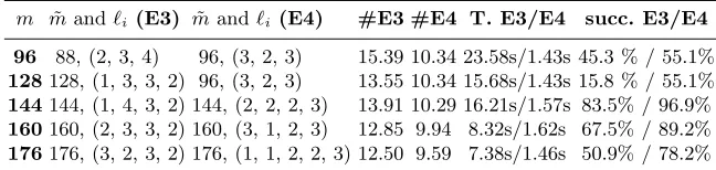
Instead of reducing the density as described in the previous section, Minder and Sinclair proposed the “extended k-tree” algorithm to make use of the extra density. When the density satisfies (3), Min-der and Sinclair use k = 2t (In the previous section, the CPW algorithm chooses k = 2t−1) by choosing appropriate subgroups Hi. Let ℓi ≥ 1 be chosen later, subject to ℓ1+ℓ2+· · ·+ℓt = n. The subgroup
H1 = {(0,· · ·,0, gℓ1+1,· · ·, gn)T : gi ∈ Zq} such that G/H1 ∼= Zℓ1q corresponds to the first ℓ1 positions of the vector. Similarly, H2 = {(g1,· · · , gℓ1,0,· · ·,0, gℓ1+ℓ2+1,· · · , gn) : gi ∈ Zq} such that G/H2 ∼= Zℓ2q corresponds to the next ℓ2 positions of the vector. Finally, Ht ={(g1,· · · , gℓ1+···+ℓt−1,0,· · ·,0) :gi ∈Zq} corresponds to the last ℓt positions of the vector. Denote by L(i) any of the lists at the i-th stage of the algorithm. The time complexity for Minder and Sinclair’s algorithm is ˜O(2t
·max0≤i≤t(#L(i))). To minimise
the running time, one needs to minimise max0≤i≤t(#L(i)). The expected size of the lists on each level is
#L(i)= #L(i−1)#L(i−1)/qℓi,1
≤i≤t.
Write #L(i)= 2bi where b
0=mlog2(#B)/2t, bi= 2bi−1−log2(q)ℓi. To minimize the time complexity, one computes the optimal valuesℓi by solving the following integer program.
minimize bmax= max 0≤i≤tbi subject to 0≤bi, 0≤i≤t
b0=mlog2(#B)/2t,
bi= 2bi−1−ℓilog2(q),
ℓi≥0, 0≤i≤t t
X
i=1
ℓi=n.
Theorem 3.1 in [20] shows that the solution to the above linear program (i.e., removing the constraint
ℓi ∈Z) is ℓ2 =· · · =ℓt−1 = (n−ℓ1)/tand ℓt = 2(n−ℓ1)/t where ℓ1 satisfies (#B)m/2 t
·(#B)m/2t/qℓ1 =
q(n−ℓ1)/t. This gives max
0≤i≤t(#L(i)) =q(n−ℓ1)/t. From (3), we have 0< ℓ1< n/(t+1). The time complexity of Minder and Sinclair’s algorithm is ˜O(2t·max
0≤i≤t(#L(i))) = ˜O(2t·q(n−ℓ1)/t).6 It follows that
(#B)m/2t < max 0≤i≤t(#L
(i)) =q(n−ℓ1)/t<(#
B)m/2t−1.
At a high level, Minder and Sinclair make use of the extra density in the instance to add one more level that eliminatesℓ1 coordinates. The time complexity for Minder and Sinclair’s refinement of CPW is better than the original version described in the previous section since ˜O(2t
·q(n−ℓ1)/t)<O˜(2t
·(#B)m/2t−1 ) and ˜
O(2t·q(n−ℓ1)/t)<O˜(2t·qn/t).
2.7 The algorithm of Howgrave-Graham and Joux (HGJ)
We now present the HGJ algorithm, that can be applied even for instances of the (G, m,B)-ISIS problem of density≤1. The algorithm heuristically improves on the square-root time complexity of Schroeppel-Shamir. For simplicity we focus on the caseB={0,1}. Section 6 of [12] notes that a possible extension is to develop the algorithm for “vectorial knapsack problems”. Our formulation contains this predicted extension.
The first crucial idea of Howgrave-Graham and Joux [12] is to split the vectorxby weight rather than by positions. The second crucial idea is to reduce to a simpler problem and then apply the algorithm recursively. The procedures in [12] use reduction moduloM, which we generalise as a map into a quotient groupG/H. It follows that the HGJ algorithm can be applied to a more general class of problems.
Supposes=Axin Gwhere x∈ Bm has weight wt(x) =ω. Our goal is to computex. Write
X for the set of weightωvectors inBm, and write
X1,X2for the set of weightω/2 vectors inBm. Then there are ω/ω2 ways to writexasx1+x2 wherex1∈ X1,x2∈ X2.
The procedure is to choose a suitable subgroupH so that there is a good chance that a randomly chosen elementR∈G/H can be written asAx1 for one of the ω/ω2choices forx1. Then the procedure solves the two subset-sum instances in the groupG/H (recursively) to generate lists of solutions
L1={x1∈ Bm:Ax1=R (modH),wt(x1) =ω/2}
and
L2={x2∈ Bm:Ax2=s−R (mod H),wt(x2) =ω/2}.
6
We actually store pairs of values (x1,Ax1 (modH′))∈ Bm×(G/H′) for a suitably chosen subgroupH′. One then applies Algorithm 1 to merge the lists to get solutionsx=x1+x2∈ X satisfying the equation in
G/(H∩H′). The paper [12] gives several solutions to the problem of merging lists, including a 4-list merge. But the main algorithm in [12] exploits Algorithm 1.
The subgroup H is chosen to trade-off the probability that a random value R corresponds to some splitting of the desired original solutionx(this depends on the size of the quotient groupG/H), while also ensuring that the listsL1 andL2 are not too large.
The improvement in complexity for finding the solutions inL1andL2is due to the lowering of the weight fromω toω/2. This is why the process is amenable to recursive solution. At some point one terminates the recursion and solves the problem by a more elementary method (e.g. Schroeppel-Shamir).
One inconvenience is that we may not know exactly the weight of the desired solutionx. If we can guess that the weight of xlies in [ω−2ǫ, ω+ 2ǫ] then we can construct lists{x1 :Ax1 =R (mod H),wt(x1)∈ [ω/2−ǫ, ω/2 +ǫ]}. A similar idea can be used at the bottom level of the recursion, when we apply the Schroeppel-Shamir method and so need to split into vectors of half length and approximately half the weight.
One must pay attention to the relationship between the group G/H and the original group G. For example, when solving modular subset-sum inG=Zq whereqdoes not have factors of a suitable size then, as noted in [12], “we first need to transform the problems into (polynomially many instances of) integer knapsacks”. For the caseG=Znq this should not be necessary.
Complexity analysis The final algorithm is a careful combination of these procedures, performed recursively. We limit our discussion to recursion of 3 levels. In terms of the subgroups, the recursive nature of the algorithm requires a sequence of subgroupsH1, H2, H3 (of similar form to those in Section 2.5, but we now requireH1∩H2∩H36={0}) so that the quotient groupsG/(H1∩H2∩H3),G/(H2∩H3),G/H3become smaller and smaller. The “top level” of the recursion turns an ISIS instance inG to two lower-weight ISIS instances inG′=G/(H
1∩H2∩H3); to solve these sub-instances using the same method we need to choose a quotient of G′ by some proper subgroup H
2∩H3, which is the same as taking a quotient of G by the subgroupH2∩H3 etc.
In [12], for subset-sum overZ, this tower of subgroups is manifested by taking moduliM that divide one another (“For the higher level modulus, we chooseM = 4194319·58711·613”, meaning H3 = 613Z, H2= 58711Z, H1 = 4194319Z, H2∩H3 = (58711·613)Z and H1∩H2∩H3 = MZ). In the case of modular subset-sum in Zq when q does not split appropriately one can lift to Z (giving a polynomial number of instances) and reduce each of them by a new composite modulus.
We do not reproduce all the analysis from [12], since it is superseded by the method of Becker et al. But the crucial aspect is that the success of the algorithm depends on the probability that there is a splitting
x = x1+x2 of the solution into equal weight terms such that Ax1 = R (modH). This depends on the number ω/ω2
of splittings of the weight ω vectorx and on the size M = #(G/H) of the quotient group. Overall, the heuristic running time for the HGJ method to solve the (I)SIS problem when ω = m/2 (as stated in Section 2.2 of [2]) is ˜O(20.337m).
2.8 The algorithm of Becker, Coron and Joux
Becker, Coron and Joux [2] present an improved version of the HGJ algorithm (again, their paper is in the context of subset-sum, but easily generalises to our setting). The idea is to allow larger coefficient sets. Precisely, supposeB={0,1}and letX ⊂ Bmbe the set of weightωvectors. The HGJ idea is to split
We briefly sketch the heuristic analysis from [2] for the case of 3 levels of recursion,B={0,1},G=Znq, and where we solve ISIS instances of density 1 (so that 2m
≈qn) with a solution of weightm/2. Let
Xa,b={x∈ {−1,0,1}m: #{i:xi= 1}=am,#{i:xi=−1}=bm}.
A good approximation to #Xa,bis 2H(a,b)·mwhereH(x, y) =−xlog2(x)−ylog2(y)−(1−x−y) log2(1−x−y). Choose subgroups H1, H2, H3 (of the similar form to Section 2.6) such that #(G/Hi) = qℓi. Fix α= 0.0267, β = 0.0168 and γ = 0.0029 and also integers ℓ1, ℓ2, ℓ3 such that qℓ1 ≈ q0.2673n = 20.2673m, qℓ2 ≈ 20.2904mandqℓ3 ≈20.2408m. Note that #(G/(H
1∩H2∩H3))≈q0.2015n≈20.2015m.
Theorem 1. (Becker-Coron-Joux) With notation as above, and assuming heuristics about the pseudoran-domness of Ax, the BCJ algorithm runs in time O˜(20.2912m).
Proof. (Sketch) The first level of recursion splits X = Bm into
X1+X2 where X1 = X2 =X1/4+α,α. We compute two lists L(1)1 ={(x,Ax) : x ∈ X1,Ax ≡R1 (mod H1∩H2∩H3)} and L(1)2 , which is the same exceptAx≡s−R1 (modH1∩H2∩H3). The expected size of the lists is 2H(1/4+α,α)m/qℓ1+ℓ2+ℓ3 = 20.2173m and merging requires ˜O((20.2173m)2/qn−ℓ1−ℓ2−ℓ3)= ˜O(20.2331m) time.
The second level of recursion computes each of L(1)1 and L (1)
2 , by splitting into further lists. For ex-ample, L(1)1 is split into L
(2)
1 = {(x,Ax) : x ∈ X1/8+α/2+β,α/2+β,Ax ≡ R2 (mod H2∩H3)} and L(2)2 is similar except the congruence is Ax ≡R1−R2 (modH2∩H3). Again, the size of lists is approximately 2H(1/8+α/2+β,α/2+β)m/qℓ2+ℓ3 = 20.2790mand the cost to merge is ˜O(22·0.2790m/qℓ1) = ˜O(2(2·0.2790−0.2673)m) =
˜
O(20.2907m).
The final level of recursion computes eachL(2)j by splitting into two lists corresponding to coefficient sets
X1/16+α/4+β/2+γ,α/4+β/2+γ. The expected size of the lists is
2H(1/16+α/4+β/2+γ,α/4+β/2+γ)m/qℓ3 ≈20.2908m
and they can be computed efficiently using the Shroeppel-Shamir algorithm in time
˜
O(p2H(1/16+α/4+β/2+γ,α/4+β/2+γ)m) = ˜O(20.2658m).
Merging the lists takes ˜O(22·0.2908/qℓ2) = ˜O(20.2912m) time. Thus the time complexity of the BCJ algorithm is ˜O(20.2912m).
The above theorem does not address the probability that the algorithm succeeds to output a solution to the problem. The discussion of this issue is complex and takes more than 3 pages (Section 3.4) of [2]. We give a rough “back-of-envelope” calculation that gives some confidence.
Suppose there is a unique solution x ∈ {0,1}m of weightm/2 to the ISIS instance. Consider the first step of the recursion. For the whole algorithm to succeed, it is necessary that there is a splittingx=x1+x2 of the solution so that x1 ∈L(1)1 and x2 ∈ L(1)2 . We split x so that the m/2 ones are equally distributed acrossx1 andx2, and them/2 zeroes are sometimes expanded as (−1,+1) or (+1,−1) pairs. We call such splittings “valid”. Hence, the number of ways to splitxin this way is
N1=
m/2
m/4
m/2
αm
(1/2−α)m αm
=
m/2
m/4
m/2
αm, αm,(1/2−2α)m
. (4)
For randomly chosenR1∈G/(H1∩H2∩H3), there is a good chance that a valid splitting exists ifN1≥
qℓ1+ℓ2+ℓ3. Indeed, the expected number of valid splittings should be roughly
N1/qℓ1+ℓ2+ℓ3. Hence, we choose
N1≈qℓ1+ℓ2+ℓ3 to make sure a valid splitting exists at this stage with significant probability.
For the second stage we assume that we already made a good choice in the first stage, and indeed that we haveN1/qℓ1+ℓ2+ℓ3 possible values forx1. The number of ways to further splitx1is
N2=
(1/4 +α)m
(1/8 +α/2)m
αm
αm/2
(3/4
−2α)m βm, βm,(3/4−2α−2β)m
The expected number of valid splittings at this stage should be roughly (N1/qℓ1+ℓ2+ℓ3)(N2/qℓ2+ℓ3)2. For ran-domly chosenR2∈G/(H2∩H3), there is a good chance to have a valid splitting if (N1/qℓ1+ℓ2+ℓ3)(N2/qℓ2+ℓ3)2≥ 1 (remember that this stage requires splitting two solutions from the first stage). Hence, we choose N1 ≈
qℓ1+ℓ2+ℓ3,N
2≈qℓ2+ℓ3.
In the final stage (again assuming good splittings in the second stage), the number of ways to split is
N3=
(1/8 +α/2 +β)m
(1/16 +α/4 +β/2)m
(β+α/2)m
(β/2 +α/4)m
(7/8−α−2β)m γm, γm,(7/8−α−2β−2γ)m
.
The expected number of valid splittings is (N1/qℓ1+ℓ2+ℓ3)(N2/qℓ2+ℓ3)2(N3/qℓ3)4, which we require to be≥1. Hence, we chooseN1≈qℓ1+ℓ2+ℓ3,N2≈qℓ2+ℓ3,N3≈qℓ3. Thus, choosing #G/H3close toN3, #G/(H2∩H3) close toN2 and #G/(H1∩H2∩H3) close toN1then it is believed the success probability of the algorithm is significantly larger than 0. This argument is supported in Section 3.4 of [2] by theoretical discussions and numerical experiments. To conclude, for the algorithm to have a good chance to succeed we require
N1/qℓ1+ℓ2+ℓ3 ≥1, (N1/qℓ1+ℓ2+ℓ3)(N2/qℓ2+ℓ3)2≥1,
(N1/qℓ1+ℓ2+ℓ3)(N2/qℓ2+ℓ3)2(N3/qℓ3)4≥1.
2.9 Summary
Despite the large literature on the topic, summarised above, one sees there are only two fundamental ideas that are used by all these algorithms:
– Reduce modulo subgroups to create higher density instances.Since the new instances have higher density one now has the option to perform methods that only find some of the possible solutions.
– Splitting solutions.Splitting can be done by length (i.e., positions) or by weight. Either way, one reduces to two “simpler” problems that can be solved recursively and then “merges” the solutions back to solutions to the original problem.
The main difference between the methods is that CPW requires large density to begin with, in which case splitting by positions is fine. Whereas HGJ/BCJ can be applied when the original instance has low density, in which case it is necessary to use splitting by weight in order to be able to ignore some potential solutions.
3
Analysis of HGJ/BCJ in high density
The CPW algorithm clearly likes high density problems. However, the analysis of the HGJ and BCJ algo-rithms in [12, 2] is in the case of finding a specific solution (and so is relevant to the case of density at most 1). It is intuitively clear that when the density is higher (and so there is more than one possible solution), and when we only want to compute a single solution to the problem, then the success probability of the algorithm should increase. In this section we explain that the parameters in the HGJ and BCJ algorithms can be improved when one is solving instances of density>1. This was anticipated in [13]: “further improve-ments can be obtained if, in addition, we seek one solution among many”. We now give a very approximate heuristic analysis of this situation. We focus on the caseB={0,1}mandG=Zn
q. As with previous work, we are not able to give general formulae for the running time as a function of the density, as the parameters in the algorithms depend in subtle ways on each other. Instead, we fix some reference instances, compute optimal parameters for them, and give the running times.
The standard approach is to choose the subgroupsH1, H2,· · · , Htsuch that #G/(Hi∩Hi+1∩· · ·∩Ht) =
qℓi+ℓi+1+···+ℓt ≈ N
i for all 1≤i≤t. The success probability is then justified by requiring
N1
qℓ1+···+ℓt
N2
qℓ2+···+ℓt
2
· · ·
Ni
qℓi+···+ℓt
2i
−1
≥1
for all 1 ≤i ≤t. We now assume a best-case scenario, that all the splittings of all the Nsol ≥1 solutions are distinct. This assumption is clearly unrealistic for large values of Nsol, but it gives a rough idea of how much speedup one can ask with this approach. We address this assumption in Section 3.1. Then the success condition changes, for all 1≤i≤t, to
Nsol N1
qℓ1+···+ℓt
N2
qℓ2+···+ℓt
2
· · ·
Ni
qℓi+···+ℓt
2i
−1
≥1. (5)
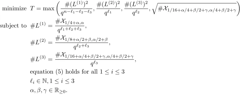
It follows that, for example when t = 3 the best parameters ℓ1, ℓ2, ℓ3, α, β, γ are chosen by the following integer linear program.
minimize T = max
#(L(1))2
qn−ℓ1−ℓ2−ℓ3,
#(L(2))2
qℓ1 ,
#(L(3))2
qℓ2 ,
q
#X1/16+α/4+β/2+γ,α/4+β/2+γ
subject to #L(1)= #X1/4+α,α
qℓ1+ℓ2+ℓ3 ,
#L(2)= #X1/8+α/2+β,α/2+β
qℓ2+ℓ3 ,
#L(3)= #X1/16+α/4+β/2+γ,α/4+β/2+γ
qℓ3 ,
equation (5) holds for all 1≤i≤3
ℓi∈N,1≤i≤3
α, β, γ∈R≥0.
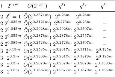
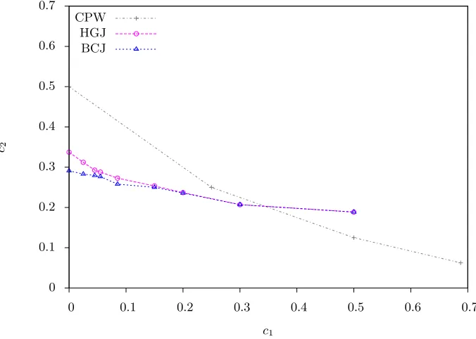
For the ISIS problem B ={0,1}mgiven q andn, the density is 2m/qn. For a given density 2c1m one can estimate the time complexity as ˜O(2c2m) by solving the above linear program and choosing the optimal parametersα, β, γandℓ1, ℓ2, ℓ3. We use LINGO 11.0 to do the optimization and obtain Table 2 and 3 giving calculations for HGJ/BCJ. For comparison we recall in Table 1 the results of Sections 2.5 and 2.6 on the time complexity of CPW. We draw Figure 1, which indicates how the density affects the asymptotic complexity for CPW7, HGJ and BCJ.
Table 1.Time complexity of CPW for different density.
t 2c1m O(2˜ c2m) 1 1 O(2˜ 0.5m
) 2 20.25m O(2˜ 0.25m) 3 20.5m O(2˜ 0.125m) 4 20.6875m ˜
O(20.0625m
)
7
Table 2.Time complexity of HGJ for different density.
t 2c1m O(2˜ c2m) qℓ1 qℓ2 qℓ3 2 20
= 1 ˜O(20.3371m) 20.25m 20.25m – 2 20.025m ˜
O(20.3121m
) 20.275m
20.25m
– 2 20.045mO(2˜ 0.2928m) 20.2928m 20.2507m – 2 20.055mO(2˜ 0.2878m) 20.2878m 20.2557m – 2 20.085m ˜
O(20.2728m
) 20.2728m
20.2707m
– 3 20.15m O(2˜ 0.2535m) 20.2617m 20.1711m 20.125m 3 20.2m O(2˜ 0.2368m) 20.2617m 20.1878m 20.125m 3 20.3m ˜
O(20.2070m
) 20.2670m
20.2070m
20.1303m
3 20.5m O(2˜ 0.1887m) 20.2677m 20.1879m20.1669m
Table 3.Time complexity of BCJ for different density.
t 2c1m O(2˜ c2m) qℓ1 qℓ2 qℓ3 α β γ 3 20
= 1 ˜O(20.2912m) 20.2673m20.2904m20.2408m 0.0267 0.0168 0.0029 3 20.025m ˜
O(20.2829m
) 20.2463m
20.2802m
20.2829m
0.02578 0.01973 0.00534 3 20.045mO(2˜ 0.2794m) 20.2604m20.2794m20.2770m0.02818 0.01833 0.00453 3 20.055mO(2˜ 0.2765m) 20.2634m20.2765m20.2649m0.02651 0.01705 0.00391 3 20.085m ˜
O(20.2579m
) 20.2404m
20.2564m
20.1818m
0.01082 0.00888 0.00131 3 20.15m O(2˜ 0.2499m) 20.2430m20.2499m20.1554m0.00102 0.00971 0.00023 3 20.2m O(2˜ 0.2357m) 20.2357m20.2358m20.2036m0.00231 0.01171 0.00206 3 20.3m ˜
O(20.2070m
) 20.2670m
20.2070m
20.1303m
0 0 0
3 20.5m O(2˜ 0.1887m) 20.2677m20.1879m20.1669m 0 0 0
These results demonstrate that, although CPW is the best choice for very high density instances, the HGJ/BCJ algorithms do perform better when the density is increased and they are better than CPW for quite a large range of densities. The final rows of Table 3 show that the BCJ algorithm becomes exactly the HGJ algorithm once the density is sufficiently high.
To invert the SWIFFT hash function the parameters are B = {0,1}m, G= Zn
q, m = 1024, q = 257,
n= 64 and so the density is 20.5m. Figure 1 therefore confirms that, for this problem, the CPW algorithm is the right choice.
3.1 Heuristic Justification of Assumption
The above analysis is based on the strong simplifying assumption that all the splittings of all theNsol= 2c1m solutions are distinct, and it should not be assumed that the HGJ and BCJ algorithms perform exactly this well. However, we believe the assumption is reasonable when the density is moderate. The reason is given as follows.
We have Nsol = 2c1m solutions x ∈ Bm such that Ax = s. We suppose all these solutions look like independently chosen binary strings of Hamming weight very close tom/2. Consider one solutionx. In the first level of the recursion we splitx=x1+x2wherex1,x2∈ X1/4+α,α. There areN1ways to do this, where
N1 is given in equation (4) and all these splittings have, by definition, distinct values for x1. Turning this around, the probability that a vectorx1 ∈ X1/4+α,α appears as a splitting ofx should be p1 = #X1N/4+1α,α. Now consider splitting a second solutionx′ =x′
0 0.1 0.2 0.3 0.4 0.5 0.6 0.7
0 0.1 0.2 0.3 0.4 0.5 0.6 0.7
c2
c1
CPW HGJ BCJ
Fig. 1.Heuristic comparison of the performance of CPW, HGJ and BCJ algorithms on ISIS instances of density≥1. The horizontal axis is the valuec1 such that the density (expected number of solutions) is 2c1m. The vertical axis is
the constantc2 such that the heuristic asymptotic complexity is ˜O(2c2m).
the previous valuesx1 is p1. Hence, the total number of “new” solutions{x1,x1′}is N1+ (1−p1)N1. The following Lemma extends this argument.
Lemma 1. LetX be a set. Suppose distinct subsetsXi ofX of sizeN1 are chosen uniformly at random for 1≤i≤t. Let p=N1/#X. Then the expected size of ∪it=1Xi is(1−(1−p)t)N1/p.
Proof. The probability that any givenx∈X1 lies inX2 is p, so the expected size of X1∩X2 is p#X1. So we expect #(X1∪X2) = (2−p1)N1= (1 + (1−p))N1.
The probability that any x ∈ X1 ∪X2 lies in X3 is p, so the expected size of (X1 ∪X2)∩X3 =
p#(X1∪X2) =p(1+(1−p)). Hence, we expect #(X1∪X2∪X3) = #(X1∪X2)+#X3−#((X1∪X2)∩X3) = (1 + (1−p) + 1−p(1 + (1−p)))N1= (1 + (1−p) + (1−p)2)N1. More generally, one can show by induction that the expected value of #(X1∪ · · · ∪Xt) is (1 + (1−p) +· · ·+ (1−p)t−1)N1= 1−(1−p)
t p N1.
Lemma 1 indicates that when we split allNsol solutionsx, the total number of vectors x1 ∈ X1/4+α,α should be roughly (1−(1−p1)Nsol)N1/p1. Ifp1Nsolis very small (≪1) then one has (1−p1)Nsol ≈1−p1Nsol and so (1−(1−p1)Nsol)/p1 ≈ Nsol. In other words, almost all the splittings of all theNsol solutions are distinct. For the values of α listed in Tables 2 and 3, max(p1) = 2−0.2143m, and so if Nsol ≤20.2m then
p1Nsol ≤2−0.0143m. Hence, the assumption made earlier seems justified when the density is less that 20.2m. We now assume this is the case.
In the second level of the recursion we haveN′
sol=Nsolqℓ1 +Nℓ12 +ℓ3 solutions. Each solution hasN2splittings as a sum of vectors in X1/8+α/2+β,α/2+β. Let p2 = #X N2
1/8+α/2+β,α/2+β be the probability a random vector appears as such a splitting. Lemma 1 shows that, as long as p2Nsol′ ≪ 1, we again expect almost all the splittings to be distinct.
For all values α, β listed in Tables 2 and 3 we have max(p2) = 2−0.2469m. SinceNsolqℓ1 +Nℓ12+ℓ3 ≤ Nsol ≤ 20.2m (when
the time complexity, soqℓ1+ℓ2+ℓ3
≥ N1) it follows thatp2Nsol′ ≤2−0.0469m is very small. So the assumption is again justified in these cases.
Finally consider the third level of the recursion. The argument is the same as above. Let N′′
sol =
Nsol
N1 qℓ1 +ℓ2 +ℓ3
N2 qℓ2 +ℓ3
2
be the number solutions to be split. Let p3 = #X N3
1/16+α/4+β/2+γ,α/4+β/2+γ. For all values α, β, γ listed in Tables 2 and 3 we have max(p3) = 2−0.2123m. Since Nsol′′ ≤ Nsol ≤20.2m (when
Nsol = 1, one chooses qℓ1+ℓ2+ℓ3 ≈ N1 and qℓ2+ℓ3 ≈ N2, while if Nsol > 1, one choosesqℓ1+ℓ2+ℓ3 ≥ N1 andqℓ2+ℓ3 ≥ N
2 to reduce the time complexity),p3Nsol′′ = 2−0.0123m is very small. Thus
1−(1−p3)N ′′sol p3 N3≈
N′′
solN3, i.e., almost all the splittings of all the Nsol′′ solutions at this stage are distinct.
Hence, when the density is≤20.2m, Figure 1 is an accurate view of the complexity of the HGJ and BCJ algorithms. When the density is greater than 20.2mthen the results of Figure 1 are less rigorous, but they at least give some intuition for how the HGJ and BCJ algorithms behave. In any case, once the density reaches around 20.3mone would likely switch to the CPW algorithm.
4
Hermite normal form
We now give the main idea of the paper. For simplicity, assume thatqis prime,G=Znq andn >1. We also assume that the matrixAhas rank equal ton, which will be true with very high probability whenm≫n. We exploit the Hermite normal form. Given an n×m matrix A over Zq with rank n < m then, by permuting columns as necessary, we may assume thatA= [A1|A2] whereA1 is an invertiblen×nmatrix andA2 is ann×(m−n) matrix. Then there exists a matrixU=A−11such that
UA= [In|A′]
whereIn is the n×nidentity matrix andA′ is the n×(m−n) matrixUA2. The matrix [In|A′] is called the Hermite normal form (HNF) ofA and it can be computed (together withU) by various methods. We assumeqis prime and hence Gaussian elimination is sufficient to compute the HNF.
WritingxT = (xT
0|xT1) wherex0has length nandx1 has lengthm−nwe have that
s≡Ax (modq) if and only if s′ =Us≡A′x1 + x0 (mod q).
Hence, the Hermite normal form converts an ISIS instance to an instance of LWE (learning with errors) having an extremely small number of samples (n < m) and with errors chosen from B rather than from a discrete Gaussian distribution on Z. We rename (A′,s′,x0,x1) as (A,s,e,x) so the problem becomes
s=Ax+e.
It is not the goal of this paper to discuss the learning with errors problem in great detail. As with ISIS, it can be reduced to the closest vector problem in a lattice and hence solved using lattice basis re-duction/enumeration techniques. There are two other notable algorithms for learning with errors, due to Arora-Ge and Blum-Kalai-Wasserman. However, since our variant of LWE has a fixed small number of samples they cannot be applied.
We will now apply the previous algorithms for the ISIS problem to this variant of the problem. This project was suggested in Section 6 of [12] to be an interesting problem (they called it the “approximate knapsack problem”). Our approach is to replace exact equality of elements in quotient groupsG/H =Zℓq, in certain parts of the algorithm, by an approximate equalityy1≈y2. The definition of y1≈y2 will be that
y1−y2∈ E, whereE is some neighbourhood of0. Different choices ofE will lead to different relations, and the exact choice depends somewhat on the algorithm under consideration.
4.1 Approximate merge algorithm
We use similar notation to Section 2.3:X ⊆ Bm is a set of vectors, letters H
i denote suitably chosen subgroups ofGsuch that #(G/Hi) =qℓi. We split the set of vectorsX ⊆ X
1+X2={x1+x2:x1∈ X1,x2∈
X2} in some way.
We also have a set of errorsE and its splittingsE1,E2. Recall that we are trying to solves≡Ax+ewith
x∈ X ande∈ E. We also define the error setsE(i)restricted to the quotient groupsG/Hi, so that typically
E(i)=
Bℓi (For exampleE(i)={0,1}ℓi for HGJ or{−1,0,1}ℓifor BCJ).
LetH♭, H, H♯be subgroups ofGthat denote subgroups used in the CPW/HGJ/BCJ algorithms. We are merging, moduloH, partial solutions moduloH♭
∩H. For clarity, let us writeG/H♭=Zℓ′
q andG/(H∩H♭) = Zℓq+ℓ′. The input is a pair of listsL1 andL2 that are “partial solutions” moduloH♭. In other words, they are lists of pair (x,Ax) such that Ax+e ≡ s (modH♭) with e
∈ E♭
⊂ Bℓ′
(e.g., e ∈ E♭
⊂ {0,1}ℓ′
for HGJ ore∈ E♭
⊂ {−1,0,1}ℓ′
for BCJ). The goal is to output a set of solutions to the problemAx+e≡s
(modH ∩H♭) for x
∈ X and, re-using notation, e ∈ E ⊂ Bℓ+ℓ′
(e.g., e ∈ E ⊂ {0,1}ℓ+ℓ′
for HGJ or
e∈ E ⊂ {−1,0,1}ℓ+ℓ′
for BCJ). We writeE♭
1,E2♭for the error sets used in the listsL1, L2;Efor the error set forG/(H♭
∩H);E′for the error set corresponding to the elements ofG/H. For future steps of the algorithm,
the output includes information aboutAx (modH♯). The details are given in Algorithm 2.
Algorithm 2Approximate merge algorithm
Input: L1={(x,Ax (modH)) :Ax+e≡R (modH♭),x∈ X1,e∈ E1♭},
L2 ={(x,Ax (modH)) :Ax+e≡s−R (modH♭),x∈ X2,e∈ E2♭}
Output: L={(x,Ax (modH♯)) :Ax+e≡s (modH∩H♭),x∈ X,e∈ E } 1: InitialiseL={}
2: SortL1 with respect to the second coordinate
3: for (x1,u)∈L2 do
4: Computev=s−u (modH)
5: for(x2,u′)∈L1withv≈u′(i.e.,u′−v∈ E′)do
6: if x1+x2∈ X andA(x1+x2)≈s (modH∩H♭)then
7: ComputeA(x1+x2) (modH♯)
8: Add (x1+x2,A(x1+x2) (modH♯)) toL
The detection of valuesu′ in the sorted list such thatv
≈u′ (meaningu′
−v=efor somee∈ E′) can
be done in several ways. One is to try all possible error vectors eand look up each candidate valuev+e. Another is to “hash” using most significant bits. We give the details below. The running time of the algorithm depends on this choice. For each match we check the correctness for the whole quotientG/(H∩H♭).
Lemma 2. Let G/H=Zℓq and letE′⊆Zℓq be an error set forG/H. Algorithm 2 performs
˜
O #L1log(#L1) + #L2
#L1/(qℓ/#E′)
operations.
Proof. SortingL1 takes ˜O(#L1log(#L1)) operations on vectors in G/H=Zℓq.
For each pair (x1,u)∈L2 and eache∈ E′ ⊆Zℓq, the expected number of “matches” (x2,u−e) inL1 is #L1/qℓ. In the case where all values fore∈ E′ are chosen and then each candidate foru′ is looked up in the table, then the check in line 6 of the algorithm is performed
#L2#E′
#L1
qℓ
.
In the BCJ application in Section 4.3 we will always have #L1 ≥qℓ. Hence we can ignore the ceiling operation in the ˜O(#L1#L2/(qℓ/#E′)) term.
As previously, it is non-trivial to bound the size of the output listL. Instead, this can be bounded by #X#E/#(G/(H∩H♭)).
Note that different choices forE,E♭
1,E2♭,E′can lead to different organisation in the algorithm. For example we may take the possible non-zero positions in E♭
1 and E2♭ to be disjoint, then after executing line 5 of Algorithm 2 we always have A(x1+x2)≈ s (mod H♭), and so in line 6 of Algorithm 2 we only need to checkA(x1+x2)≈s (mod H) – this is what we will do when adapting the CPW algorithm to this case.
4.2 The CPW algorithm
Recall that our problem is (taking the HNF and then renaming (A′,s′) as (A,s) and denoting (x
1,x0) as (x,e)): Given A, q,sto solve Ax+e=s in G =Znq, where x has length m−n ande has length n. We assume the problem has high density, in the sense that there are many pairs (x,e) ∈ Bm that solve the system.
As we have seen, the CPW algorithm is most suitable for problems with very high density, since higher density means more lists can be used and so the running time is lower. Hence, it may seem that reducingm
to m−n will be unhelpful for the CPW algorithm. However, we actually get a very nice tradeoff. In some sense, the high density is preserved by our transform while the actual computations are reduced due to the reduction in the size ofm.
As noted, we define a (not-necessarily symmetric or transitive) relation≈on vectors inG=Znq asv≈w if and only ifv−w∈ Bn. One can then organise a CPW-style algorithm: compute the lists L(i)
j as usual, but merge them using≈. However, we need to be a bit careful. Consider the case of four lists. Lists L(0)j contain pairs (x,Ax) (in the case ofL(0)4 it is (x,Ax−s)). MergingL(0)1 andL(0)2 gives a listL(1)1 of pairs (x1+x2,A(x1+x2) (modH2)) for x1 ∈L(0)1 and x2 ∈L(0)2 such thatA(x1+x2)≈0 (modH1), which meansA(x1+x2)≡e (mod H1) for some e∈ Bn/3. Similarly, L(1)2 is a list of pairs (x1+x2,A(x1+x2) (modH2)) for x1 ∈L(0)3 andx2 ∈L(0)4 such thatA(x1+x2)−s≡e′ (modH1) for some e′ ∈ Bn/3. The problem is thate+e′ does not necessarily lie in
Bn/3and so the merge at the final stage will not necessarily lead to a solution to the problem.
There are several ways to avoid this issue. One would be to “weed out” these failed matches at the later stages. However, our approach is to constrain the relation≈further during the merge operations. Specifically (using the notation of the previous paragraph) we require the possible non-zero positions ine ande′ to be
disjoint.
The details. To be precise, let k = 2t be the number of lists. We define u = (m
−n)/k and let Xj =
{(0, . . . ,0, x(j−1)u+1, . . . , xju,0, . . . ,0) ∈ Bm−n} for 1 ≤ j ≤ k. It turns out to be better to not have all merges using quotient groups of the same size, so we choose integersℓi>0 such thatℓ1+ℓ2+· · ·+ℓt=n. We will choose the subgroupsHi so thatG/Hi ∼=Zqℓi for 1≤i≤t. SoH1={(0,0,· · ·,0, gℓ1+1,· · ·, gn)∈Znq},
H2={(g1, . . . , gℓ1,0, . . . ,0, gℓ1+ℓ2+1, . . . , gn)}and so on.
Letγi=ℓi/2t−i=ℓi/(k/2i). For 1≤j≤k/2i we define error setsEγ(ii),j⊆ B
ℓi restricted to the quotient groupG/Hi and withγi error positions as
Eγ(ii),j={(0, . . . ,0, e(j−1)γi+1, . . . , ejγi,0,0, . . . ,0)∈ B ℓi
}.
Note that #Eγ(ii),j= (#B) γi.
Level 0: Compute lists L(0)j ={(x,Ax (modH1))∈ Xj×Zℓ1q } for 1≤j ≤k−1 and L (0)
k ={(x,Ax−s (modH1))∈ Xk×Zℓ1q }. Note that #L
(0)
j = #Bu = #B(m−n)/k. The cost to compute the initialk lists is
O(#L(0)j ) =O((#B)(m−n)/k) or, to be more precise, the cost is approximatelyk·#L (0)
j ·C bit operations, where C is the number of bit operations to compute a sum of at most u vectors in Zℓ1q i.e. C = (m−
Level 1: We now merge the k = 2t lists in pairs to get k/2 = 2t−1 lists. Let γ
1 = ℓ1/(k/2). For j = 1,2,· · · , k/2 the setsEγ1,j(1) ∈ Bℓ1 specify the positions that are allowed to contain errors. In other words, for
j= 1,2,· · · , k/2−1 we construct the new lists
L(1)j ={(x1+x2,A(x1+x2) (modH2)) :x1∈L(0)2j−1,x2∈L(0)2j,
A(x1+x2) (modH1)∈ Eγ1,j(1) },
and
L(1)k/2={(x1+x2,A(x1+x2) (modH2)) :x1∈L(0)k−1,x2∈L(0)k ,
A(x1+x2)−s (mod H1)∈ Eγ1,k/(1) 2}.
The probability that two random vectors in Zℓ1q have sum in Eγ1,j(1) is #Eγ1,j(1) /qℓ1 = #Bγ1/qℓ1, and so the heuristic expected size of the listsL(1)j is #L
(0) 2j−1#L
(0)
2j#Bγ1/qℓ1 ≈#B2(m−n)/k+γ1/qℓ1.
Leveli≥2: The procedure continues in the same way. We are now mergingk/2i−1lists to getk/2ilists. We do this by checkingℓi coordinates and so will allow errors for each merge in only γi=ℓi/(k/2i) positions. Hence, forj = 1,2,· · ·, k/2i
−1 we construct the new lists
L(ji)={(x1+x2,A(x1+x2) (modHi+1)) :x1∈L(i
−1)
2j−1,x2∈L(i
−1) 2j ,
A(x1+x2) (modHi)∈ Eγ(ii),j},
and
L(k/i)2i ={(x1+x2,A(x1+x2) (modHi+1)) :x1∈Lk/(i−21)i−1−1,x2∈L (i−1) k/2i−1,
A(x1+x2)−s (mod Hi)∈ Eγ(ii),k/2i}.
As before, the heuristic expected size ofL(ji) is #L2(ij−−1)1#L (i−1)
2j #Bγi/qℓi.
It remains to explain how to perform the merging of the lists using Algorithm 2. We are seeking a match on vectors inZℓi
q that are equal on all butγi coordinates, and that are “close” on thoseγi coordinates. The natural solution is to detect matches using the most significant bits of the coordinates (this approach was used in a similar situation by Howgrave-Graham, Silverman and Whyte [11]). Precisely, letvi be a parameter (indicating the number of most significant bits being used). RepresentZqas{0,1, . . . , q−1}and define a hash functionF :Zq →Z2vi byF(x) =⌊q/x2vi⌋. We can then extendF toZγqi (and to the whole ofZℓqi by taking the identity map on the other coordinates). We want to detect a match of the form Ax1+Ax2+e=0, which we will express as −Ax1 = Ax2+e. The idea is to compute F(−Ax1) for all x1 in the first list and store these in a sorted list. For each value ofx2 in the second list one computes all possible values for
F(Ax2+e) and checks which of them are in the sorted list.
For example, consider q = 23 = 8 and suppose we use a single most significant bit (so F : Z q →
{0,1}). Suppose−Ax1 = (7,2,4,5,6,4,0,7)T and that we are only considering binary errors on the first 4 coordinates. Then we have F(−Ax1) = (1,0,1,1,6,4,0,7). Suppose now Ax2 = (6,2,3,5,6,4,0,7). Then
F(Ax2) = (1,0,0,1,6,4,0,7). By looking at the “borderline” entries of Ax2 we know that we should also check (1,0,1,1,6,4,0,7). There is no other value to check, sinceF((6,2,3,5) + (1,1,0,1)) = (1,0,0,1) and
F((6,2,3,5) + (1,1,1,1)) = (1,0,1,1) and so the only possible values for the first 4 entries ofF(Ax2+e) are{(1,0,0,1),(1,0,1,1)}.