Statistical process control with special reference to multivariable processes and short runs

(1)

STATISTICAL PROCESS CONTROL WITH

SPECIAL REFERENCE TO MULTIVARIABLE

PROCESSES AND SHORT RUNS

Pak Fai Tang

A thesis submitted in fialfilment of the requirements for the degree of Doctor of Philosophy

Department of Computer and Mathematical Sciences Faculty of Science

Victoria University of Technology

(2)

FTS THESIS

658.562015195 TAN

30001005084969

Tang, Pak Fai

(3)

ACKNOWLEDGMENTS

I wish to express my sincere gratitude to my principal supervisor, Associate

Professor Neil Bamett and co-supervisor. Associate Professor Peter Cerone for helpfiil

suggestions, advice, guidance and encouragement throughout this project.

Special thanks are also due to Associate Professor Ian Murray and his wife

Glenice for their warm hospitality during my stay in AustraUa, Dr. Ng Lay Swee, the

principal of Tunku Abdul Rahman College, Malaysia for her advice and encouragement,

the Department of Computer and Mathematical Sciences, Victoria University of

Technology for the financial support given to me, and Tunku Abdul Rahman College for

the study leave period granted.

I am also indebted to the staff of the Department, particularly, Tom Peachey, Neil

Diamond, Alan Glasson, Ian Gomm, Ted Alwast, P.Rajendran (Raj) and Damon

Burgess, and my fellow colleagues, particularly, Mehmet Tat, Gregory Simmons,

Violetta Misiorek, Kevin Liu, Fred Liu, Rafyul Fatri, Phillip Tse and Simon So, who

have, in one way or another, rendered their kind assistance.

(6)

DECLARATION

I hereby declare that:

(i) the following thesis contains only my original work which has not been

submitted previously, in whole or in part, in respect of any other academic

award, and

(ii) due acknowledgment has been made in the text of the thesis to all other material

used.

CpakFSr^g

(7)

ABSTRACT

The quest for control and the subsequent pursuit of continuous quality

improvement in the manufacturing sector, due to mcreasingly keen competition, has

stimulated interest in statistical process control (SPC). Whilst traditional SPC techniques

are well suited to the mass production industries, their usefiilness in short run or low

volume manufacturing environments is questionable. The major problem with short-run

SPC is lack of data for estimation of the control parameters. In view of this limitation,

many alternatives and adaptations of existing techniques have been devised. However,

these efforts have largely been devoted to monitoring and controlling univariate

processes.

In practice, the quality of manufactured products is oflien determined by reference

to several quality characteristics which are correlated. Under these circumstances, it is

necessary to use multivariate quality control procedures which take the correlational

structure into consideration. Although this area has received considerable attention in the

literature, most of the published work assumes that prior information about the process

parameters is available. This assumption is rarely the case in the short run environment.

(8)

production, whether or or not prior information about the process parameters is

available.

The techniques presented for controlling the mean vector of multivariate

processes utiUze the probability integral transformation technique in order to produce

sequences of independent or approximately independent standard normal variables. This

offers greater flexibility than the 2-stage procedures recommended by some authors in

the design of control charts for the unknown parameter case. Apart fi-om the

conventional rule that signals when a plotted value exceeds either of the 3-sigma limits,

run tests as well as the methods of Cumulative Sum (CUSUM) and Exponentially

Weighted Moving Average (EWMA) can be used. A simulation study indicates that the

techniques, with the usual decision rule imposed, are particularly usefiil for 'picking up' a

persistent change in the process mean vector when subgroup data are used, even if prior

information about the process parameters is not available. For detecting step shifts and

linear trends based on individual observations, two specifically designed EWMA charts

based on similarly transformed variables but which use a different estimator of the

process variance-covariance matrix are found to be much more effective than other

competing procedures.

(9)

control chart, for the known parameters case, is more sensitive to certain shifts than that

which involves separate charting of the standardized variances of the principal

components or the individual variables resuhing from the partitioning of the

variance-covariance matrices. The proposed techniques also possess some practical advantages

over existing procedures. In particular, better control over the false signal rate, ease of

locating control limits and identification of the nature of process changes.

To satisfactorily describe the capability of multivariate processes, a multivariate

capability index is required. This thesis describes three approaches to designing capability

indices for multivariate normal processes. Three process capability indices are presented

and some simple rules provided for interpreting the ranges of values they take. The

development of one index involves the projection of a process ellipse, containing at least

a specified proportion of products, on to its component axes. The other two are based on

Bonferroni and Sidak's multivariate normal probability inequalities in their constructions.

A comparison indicates that the latter two are superior to the former and that the

Sidak-type capability index is marginally better than that based on the Bonferroni Inequality. An

approximate test is developed for the Sidak-type capability index. A possible method of

forming robust multivariate capability indices based on multivariate Chebyshev-type

inequalities is also considered.

(10)

List of Figures

1.1 A Typical Control Chart 2

3.1 Multivariate Control Charts for Example 3.4.1 66

3.2 Multivariate Control Charts for Example 3.4.2 68

3.3 Multivariate Control Charts for Example 3.4.3 70

(a) Known Parameters

(b) Unknown Parameters

3.4 Multivariate Control Chart for Example 3.4.4

(a) Known Parameters 72

(b) Unknown Parameters 73

3.5 Multivariate Control Chart for Holmes and Mergen' s (1993) Data 77

3.6 EWMAZIU Chart for Holmes and Mergen's (1993) Data 90

3.7 EWMAZ1, EWMAZ1U and M Charts for Bivariate Data with Linear

Trend 92

3.8 Run Length Probabilities of EWMAZ 1, EWMAZ2, EWMAZ3 and

MCHARTforLinearTrend,/? = 2, <af=7, a = 0.03 95

(a) Trend Parameter = 0

(b) Trend Parameter = 0.1

(c) Trend Parameter = 0.2

(d) Trend Parameter = 0.5

3.9 Run Length Probabilities of EWMAZ 1, EWMAZ2, EWMAZ3 and

MCHARTforLinearTrend,/7 = 3, af=8, a = 0.02 96

(a) Trend Parameter = 0

(b) Trend Parameter = 0.1

(c) Trend Parameter = 0.2

(d) Trend Parameter = 0.5

3.10 Run Length Probabilities of EWMAZ 1, EWMAZ2, EWMAZ3 and

MCHARTforLinearTrend,/? = 5, i/= 10, a = 0.005 97

(a) Trend Parameter = 0

(b) Trend Parameter = 0.1

(c) Trend Parameter = 0.2

(d) Trend Parameter = 0.5

3.11 Run Length Probabilities of EWMAZ lU, EWMAZ2U and MCHARTU

for Linear Trend,/? = 2, <i= 7, a = 0.02 98

(a) Trend Parameter = 0

(b) Trend Parameter = 0.1

(c) Trend Parameter = 0.2

(d) Trend Parameter = 0.5

3.12 Run Length Probabilities of EWMAZIU, EWMAZ2U and MCHARTU

for Linear Trend,/? = 3, <af= 8, a = 0.01 99

(a) Trend Parameter = 0

(11)

for Linear Trend,/? = 5, <i= 10, a = 0.005 100 (a) Trend Parameter = 0

(b) Trend Parameter = 0.1 (c) Trend Parameter = 0.2 (d) Trend Parameter = 0.5

3.14 Run Length Probabilities of EWMAZl, EWMAZ2 and EWMAZ3 for

StepShift,/> = 2 104 (a) r= 10, noncentrality parameter = 1

(b) r = 10, noncentrality parameter = 2 (c) r = 10, noncentrality parameter = 3 (d) r = 20, noncentrality parameter = 1 (e) r = 20, noncentrality parameter = 2 (f) r = 20, noncentrality parameter = 3

Step Shift,/? = 3 105 (a) r= 10, noncentrality parameter = 1

(b) r = 10, noncentrality parameter = 2 (c) r= \0, noncentrality parameter = 3 (d) r = 20, noncentrality parameter = 1 (e) r = 20, noncentrality parameter = 2 (f) r = 20, noncentrality parameter = 3

Step Shift,/? = 5 106 (a) r= 10, noncentrality parameter = 1

(b) r = 10, noncentrality parameter = 2 (c) r = 10, noncentrality parameter = 3 (d) r = 20, noncentrality parameter = 1 (e) r = 20, noncentrality parameter = 2 (f) A* = 20, noncentrality parameter = 3

3.17 Run Length Probabilities of EWMAZIU and EWMAZ2U for Step Shift,

p = 2 107 (a) A* = 10, noncentrality parameter = 1

(b) r = 10, noncentrality parameter = 2 (c) r = 10, noncentrality parameter = 3 (d) r = 20, noncentrality parameter = 1 (e) r = 20, noncentrality parameter = 2 (f) r = 20, noncentrality parameter = 3

3.18 Run Length Probabilities of EWMAZIU and EWMAZ2U for Step Shift,

p = 3 108 (a) r = 10, noncentrality parameter = 1

(12)

3.19 Run Length Probabilities of EWMAZIU and EWMAZ2U for Step Shift,

p = 5 109

(a) r = 10, noncentrality parameter = 1

(b) r = 10, noncentrality parameter = 2

(c) r = 10, noncentrality parameter = 3

(d) r = 20, noncentrality parameter = 1

(e) r = 20, noncentraUty parameter = 2

(f) r = 20, noncentrahty parameter = 3

4.1 Dispersion Control Charts for Alt and Bedewi(l986)'s Data 154

(a) Known Variance-Covariance Matrix

(b) Unknown Variance-Covariance Matrix

5.1 Graphical Illustration of An Incapable Bivariate Normal Process with

MCp^ = \ 166

6.1 Pre-Control Scheme 187

6.2 Probability of Detection Within 5 Successive Samples (P) vs Mean Shift

in Multiples of Standard Deviation (k). A, B and C Denote Respectively

(13)

List of Tables

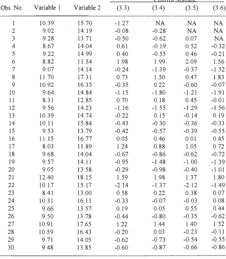
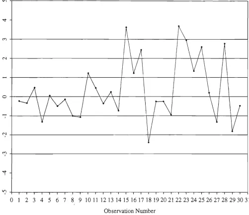
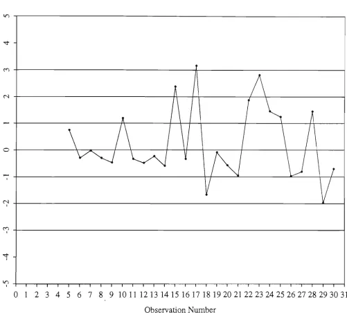
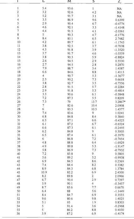
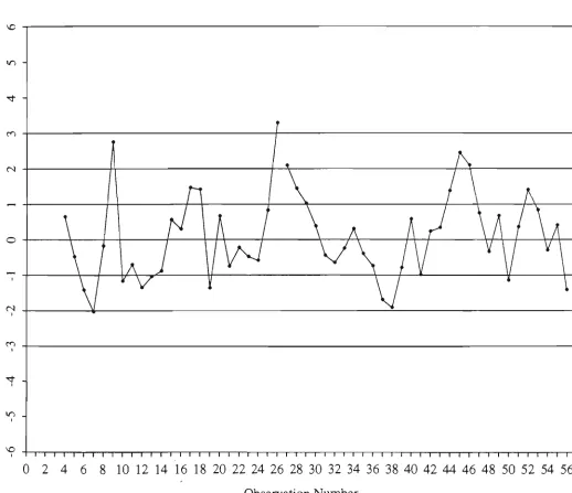
3.1 Probability of A False Signal from Any One of the First 50 Subgroups 63 3.2 Simulated Data and Values of The Control Statistics Based on

IndividualMeasurements for Example 3.4.1 65 3.3 Holmes and Mergen (1993)'s Data and Values of Statistic (3.6) 76

3.4 Values of Alt et al.(1976)'s Test Statistic, Small Sample Probability

Limits and Control Statistic (3.11) for Example 3.4.6 79 3.5 Probability of Detection Within m = 5 Subsequent Observations 84

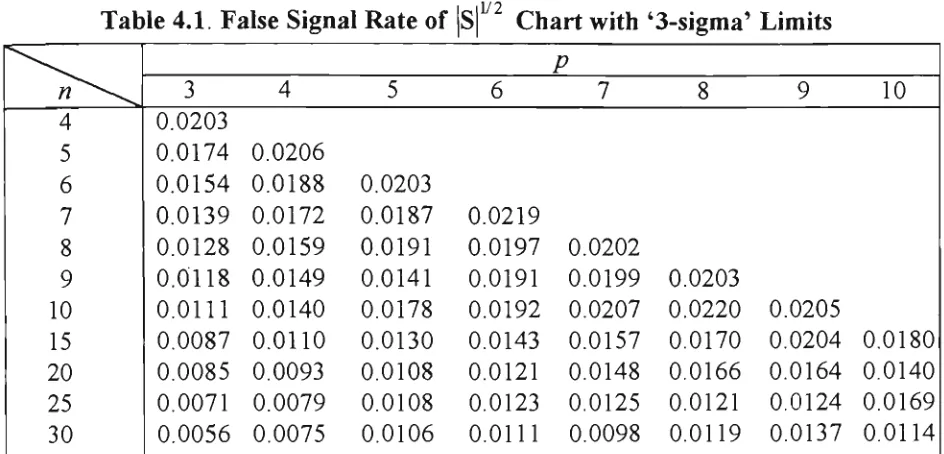
3.6 Probability of Detection Within m = 5 Subsequent Subgroups 85 4.1 False Signal Rate of |S|^^ Chart with'3-sigma'Limits 135

I i l / 2

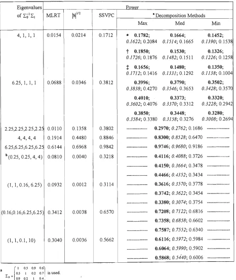
4.2 |S| Control Chart Factor, k^ 137 4.3 Power Comparison of MLRT, |S| , SSVPC and Decomposition (Proposed,

Fisher and Tippett) Techniques for/? = 3, « = 4 and a = 0.0027 142 4.4 Power Comparison of MLRT, |S| , SSVPC and Decomposition (Proposed,

Fisher and Tippett) Techniques for/? = 4, « = 5 and a = 0.0027 143 4.5 Power Comparison of MLRT, |S| , SSVPC and Decomposition (Proposed,

Fisher and Tippett) Techniques for/? = 5, « = 8 and a = 0.0027 144 4.6 Vx{RL < k) for a Change in S After the rth Subgroup, by MLRTECM and

Decomposition (Proposed, Fisher and Tippett) Techniques for/? = 2, « = 3 and

a = 0.0027 145 4.7 ¥r{RL < k) for a Change in E After the Ath Subgroup, by MLRTECM and

a = 0.0027 146 4.8 ¥r{RL < k) for a Change in E After the rth Subgroup, by MLRTECM and

a = 0.0027 147 4.9 Alt and Bedewi (1986)'s Data and Values of Control Statistic (4.14),

(4.15), MLRT Statistic (Unknown S ) a n d |S| 153 4.10 Power Comparison of Proposed, IC and ISVPC Charting Techniques for

Shifts in the Form of Zi = A,Zo 158 5.1 Relative Conservativeness of Projected, Bonferroni and Sidak-Type

Capability Indices 176 5.2 Critical Values for Testing ^Cf^ 180

6.1 Probability of Set-up Approval for Pre-Control 188

6.2 Power of Pre-Control - Mean Shift 196 6.3 Power of X Chart with 3a Limits (assumed C^ = 1) 196

6.4 Power of X Chart with Adjusted Limits (assumed C^ = l ) 197

(14)

6.7 Power of 7? Chart-Adjusted Limits (assumed Cp = 1) 198

6.8 Average Run Lengths for Pre-Control 199 6.9 Average Run Lengths for X Chart - Adjusted Limits (assumed C^ = 1) 199

6.10 Powerof X Chart (assumed C^ = 0.75) 200 6.11 Powerof ^ Chart (assumed C^ = 1.25 ) 200 6.12 Powerof X Chart (assumed C^ = 1.50 ) 201 6.13 Power ofi? Chart (assumed C^=1.25) 201 6.14 Power ofi? Chart (assumed C^=1.50) 201

6.15 A N I I M S ( P C ) 205

6.16 ANII(X) (sample size 4, control based on C^ = 1) 205

6.17 TMS 206

6.18 ANIIvi(PC) 207 6.19 ANII(i?) (sample size 4, control based on C^ = l ) 207

6.20 /vi 207 6.21 ANII(JL') (sample size 4, adjusted limits, control based on C^ = 1) 209

(15)

CHAPTER 1 INTRODUCTION

1.1 Introduction to SPC

Dr. Walter Shewhart (1931) introduced the notion of statistical process control

(SPC), and in particular control charts, as a means of monitoring industrial processes and

controlling the quality of manufactured products. These and other statistical tools have

proven usefiil in many industries.

Regardless of the nature and the state of an industrial process, any measurable

characteristics of the process or the manufactured product exhibit a certain amount of

variability. In SPC, a distinction is often made between two types of variability : one due

to common causes and the other that results from special or assignable causes.

Examples of common causes are machining operations, setting-up methods,

measurement systems and atmospheric conditions. Variability due to these factors is

either non-controllable or cannot be reduced or eliminated economically. On the other

hand, special causes include, amongst others, machine failure, tool wear, defective

material and operator error, which are preventable or at least correctable or controllable.

The primary objective of SPC is to help detect the presence of these extraneous sources

of variability so that timely corrective actions can be taken. In this manner, it is hoped

that the production process will be capable of meeting given product specifications

consistently and economically.

Once the common-cause or inherent variability has been quantified, control charts

can be used to determine when and whether or not special causes affecting the process

(16)

simply in control if it is free from the influence of such factors. Otherwise, it is said to be

out of control. In statistical terms, this means an in-control process variable has a

constant distribution. In applications, however, it is generally considered sufficient for

the process parameters such as the mean, \x and the standard deviation, a to remain

constant.

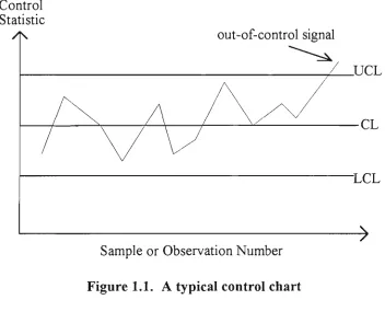
A control chart portrays the values of some chosen statistic in chronological

order and provides graphical evidence of when and whether or not process troubles

occur. As shown in Figure 1.1, a typical control chart is a plot of a control statistic

against the sample number and consists of a center line (CL), a lower control limit (LCL)

and an upper control limit (UCL).

Control Statistic

out-of-control signal

UCL

Sample or Observation Number

Figure 1.1. A typical control chart

Common examples of a control statistic are the individual observations of a quality

characteristic {X}, sample mean {X), sample range {R), sample standard deviation {S),

(17)

control Umits, which depend on the process or control parameters, act as the thresholds

for the plotted values beyond which out of control conditions are indicated. These limits

may or may not be symmetric and it is also possible that only a single control limit is used

under certain circumstances. In any event, the control Umits are usually determined such

that the resulting_^t/5e signal rate can be tolerated. A false signal occurs when the value

of the control statistic plots outside the control limits whilst in fact the process under

consideration is in control.

In practice, the control parameters are estimated based on data collected from a

process assumed to have been in control. Certain rules of thumb or practical experience

are often employed to determine the necessary amount of calibration data. The

commonly recommended approach is then to 'plug in' these sample estimates to the

formulae for the control limits. Thus, unless the set of calibration data is reasonably

large, there is often no assurance that the resulting estimated control limits will behave

essentially like the known limits (see Quesenberry (1993)).

The effectiveness of a control procedure is often determined based on its

associated run length (RL) distribution. RL refers to the number of samples taken (since

the last signal) before a signal is triggered. As a summary measure of sensitivity, the

average number of samples required for the detection of a change in the control

parameters, termed the average run length (ARL), has commonly been used. Using a

simplified ecomonic model. Ghost, Reynolds and Hui (1981) showed that ARL is the

most important measure associated with the RL distribution that determines the

effectiveness of a control procedure. They also noted that other measures may be of

interest for some applications. Quesenberry (1995d) demonstrated that for comparison of

(18)

after a shift in the process parameters, ARL is an appropriate performance criterion

because the run length distribution ftinction, 'PT[RL < k] at any fixed value k is a strictly

monotonic ftinction of ARL irrespective of shift size. On the other hand, if some of the

RL distributions are not geometric or unknown, even combining information on the

standard deviation of run length (SDRL) with ARL, as considered by some authors, may

lead to misleading conclusions about their relative performance. This issue has either

been dismissed or overlooked by numerous authors.

The idea of SPC can be extended to a more practical situation in which several

correlated quality characteristics are monitored simultaneously. Under these

circumstances, procedures which take into account the correlational structure of the

individual variables are required in order to correctly reflect the process status.

1.2 Problems of Traditional SPC for Short Production Runs

Shewhart control charts have enjoyed considerable popularity as control and

monitoring tools. These and more recent variations of them, enable production operators

to detect process troubles or out-of-control situations before they become critical.

Appropriate corrective action can then be initiated to prevent farther deterioration in

process operation and so avoid a negative impact on product quality. While these

techniques are well suited to the mass production industries, their usefiilness in low

volume manufacturing environments is subject to debate.

Besides the continuance of traditional small job shops, there has been, even in the

mass production industries, an increased demand for more frequent production changes

and a consequential proliferation of short runs. Attempts made to apply traditional

(19)

essential problems facing those seeking to provide usefiil statistical tools for application

in the short production run environment are those of machine 'warm up', control

parameter estimation and parameter changes between the manufacture of different

product types.

In short-run environments, the control limits for traditional control charts, such as

X and R charts, often cannot be located in the usual manner due to insufficient data.

Thus, one might consider estimating the control limits based on a much smaller number

of samples or subgroups than usually recommended. However, it has been adequately

demonstrated in the literature that this practice is not reliable. Amongst others,

Quesenberry (1993) provided a most reasonable evaluation of the effect of estimated

control limits on the overall run length performance for conventional X and X charts.

He showed by means of simulation, that the rate of false alarms after short runs,

increases, and much larger sets of calibration data are required so that the resulting

estimates of the control limits for these charts are practically the same as their true

values. However, these requirements can rarely be met for small batch manufacturing.

The problems of lack of process performance data are fiirther aggravated by

process 'warm up', which is perhaps the most important and yet least considered obstacle

to meaningfiil and successftil application of traditional control charts in small lot

production. This phenomenon is a common and dominant feature of short-run processes,

as instability after set-up or reset often constitutes a large proportion of production run

time. Neglecting this fact and using sample data from such a period to obtain control

limits will often lead to erroneous conclusions regarding past, current and fiiture states of

the process. Murray and Oakland (1988) demonstrated this using simulation, specifically,

(20)

will often appear to be in control, as reflected by either a standard deviation or range

chart with the usual decision rules imposed.

Another practical reality that characterizes short run environments, is the

diversity of products made. If separate control charts are maintained for each type of

product, the system becomes unwieldy.

1.3 Multivariate Quality Control

Due to the rapid development of data-acquisition and computer technology, it is

not uncommon in many industrial situations to monitor on-going performance of a

manufacturing process with respect to more than one process or product characteristics.

If the product characteristics are correlated and no consideration is made of their joint

distribution, the use of separate control charts for each of them can be misleading.

Specifically, the related variables, when studied separately, may appear to be in statistical

control but appear out of control when considered in a multivariate context.

Montgomery and Wadsworth (1972) and Alt and Smith (1990) illustrated this for the

case of /? = 2 variables. Under these circumstances, it seems necessary to consider the

use of multivariate quality control procedures which take into account the covariance

structure of the quality characteristics.

Over the last 2 decades, the problem of multivariate quality control has received

considerable attention in the literature. A review of this work can be found in Alt et

al.(1990) and Jackson (1985) and this has been updated recently by Wierda (1994) and

Lowry and Montgomery (1995). Besides the problem of lack of data for parameter

estimation in low volume and short-run environments, multivariate SPC procedures

(21)

interpreting the out-of-control signals. Other issues include use and understanding,

complexity of the distribution theory involved and statistical efficiency. Some previously

proposed procedures such as the dispersion control technique based on generalized

variance of Alt et al.(1990) are fiindamentally flawed because they are unlikely to 'pick

up' certain shifts in the dispersion parameters. The computational aspect of multivariate

control procedures can be handled by computers but other problems remain and need

fiirther investigation.

1.4 Thesis Objectives

The main thrust of this thesis is to present some multivariate quality control

procedures that can be effectively used in situations where prior estimates of the process

parameters are unavailable. For completeness, some better alternatives to existing

multivariate SPC procedures are also provided for known parameter situations. The

types of process change considered include step shift in both the process mean vector

and the variance-covariance matrix and linear trend. Some simulations, as well as

previously published data, are used to assess the practicality of the models and the

methods. Where appropriate, the relative control performance of proposed and currently

existing procedures are also evaluated.

Statistical process control is often considered with no reference to product

specifications. It merely ensures that the process under focus is in a state of statistical

control so that its behaviour is predictable under normal operating conditions. In

practice, however, the quality and the 'acceptability' of the products is determined by

conformance to given specifications. Having confirmed that the process is in control, the

(22)

conveniently summarized by an index. Whilst substantial efforts have been devoted to the

development of capability indices for univariate situations in the literature, the work on

multivariate process capability study is at a relatively rudimentary stage. In order to

satisfactorily describe the capability of multivariate processes, some indices are therefore

presented.

In addition to the above, the relative merits of the adjusted X and R charting

technique and Pre-control are provided for the univariate situation. These tools are

attractive for application in short-run environments since they do not require

accumulation of process data for computation of the control limits but instead determines

(23)

CHAPTER 2 LITERATURE REVIEW

2.1 Introduction

In view of the limitations of traditional SPC techniques, many alternatives and

adaptations of them have been devised for the express purpose of removing the barriers

between SPC and short production runs. Recently, a review of the literature on the use

of SPC in batch production has been presented by Al-Salti and Statham (1994). Much of

their article is devoted to a particular aspect of short-run SPC, namely, the use of data

transformation techniques. This chapter, however, gives a more comprehensive review of

techniques proposed for short runs along with some possible methods and provides its

own contribution to the debate. Whilst the focus is on univariate processes, wherever

appropriate consideration is also given to the multivariate environment for which little

has appeared in the literature.

It should be pointed out that process monitoring in the chemical industries (eg.

Nomikos and MacGregor (1995), Doganaksoy, Schmee and Vandeven (1996)) are, in

most cases, not applicable to short-run SPC which assumes small production volume of

the monitored product. In chemical or continuous process industries, various products or

grades of the same product are manufactured in lots or batches and production of the

same product continues, although intermittently, followed by batches of other products

or grades and so forth. Thus, adequate historical data from past succesfiil batches are

usually available for calibrating the in-control behaviour of the quality/product variables

which are usually measured once at the end of each batch run and the process variables

(24)

For ease of presentation, the techniques to be reviewed are grouped into several

general approaches and discussed under appropriate headings although there is, of

course, inevitable overlap between the groups.

2.2 Adjusting Control Limits Based On The Number of Suberoups or

Observations

In the event of only a small number of subgroups being available yet where early

control of the process is still desirable, Hillier (1964,1967,1969) and Yang and HilHer

(1970) proposed adjusting the control limits for Shewhart-type variable control charts,

both for retrospective (stage I) testing and for fiiture (stage II) control in such a way that

the predetermined probability of a type I error is preserved. A similar approach, based on

individual observations, has also been presented by Roes, Does and Schurink (1993). It

should be pointed out, however, that the limits so adjusted do not always ensure that the

resulting probability of a type I error for each fiiture subgroup is as desired. In fact, this

probability, as well as the adjusted limits, vary stochastically with the mean and the

dispersion of the calibration sample. As such, the resulting control procedure may either

be too conservative, causing delay in reacting to process troubles, or too stringent,

giving rise to too many false alarms. Note also that, as opposed to setting the limits by

the conventional method, even if the estimates of the process parameters are accurate,

the resulting control limits are wider than necessary ! Furthermore, since the estimated

control limits may not be close to the nominal values, additional run rules such as those

discussed by Nelson (1984) cannot be used indiscriminately. Other drawbacks are the

number of calculations required and the likelihood of misinterpreting the information

(25)

and stage II, as well as changing control Umits after every couple of subgroups (Ermer

and Born (1989)).

A generalization of this approach to the control of the mean vector of a

multivariate normal process, based on the well known Hotelling T^ statistic, was

presented by Alt, Goode and Wadsworth (1976) and Tracy, Young and Mason (1992)

for the cases when subgroup data and individual measurements are used respectively.

Some issues of importance regarding the use of such a composite measure to monitor the

stability of multivariate processes were raised, for example, in Hawkins (1991,1993).

More recently, Scholz and Tosch (1994) proposed updating the parameter

estimates and the stage II control Umits for the individual values charts based on the

student-t statistic and T^ charts respectively after every fiiture observation. In order to

reduce the effect of any systematic process behaviour on the estimates of the dispersion

parameters, they suggested using a moving variance of successive observations for the

individual values chart and an analogous procedure for estimating the in-control process

variance-covariance matrix, E that is required for computing the value of the T^

statistic. The latter procedure uses vector differences of successive observations to form

the estimator of S as foUows

;-1 " "

^" ~ 2(n I) ^ '^^'^^ ~ ^/)(^/+i ~ ^ / )

2(«-l)t,

where X, and n denote respectively the /th observation vector and the number of

previous observation vectors. This estimator was considered by Holmes and Mergen

(1993) and compared to other estimators including the usual sample covariance matrix

(26)

demonstrated that, step shifts in the mean vector and linear trends are more likely to be

detected with the use of this estimator.

King (1954) has also presented a similar approach for analysis of past data or

retrospective testing using X charts with control limits based on average subgroup

range except that the control chart factors are derived in such a way that the joint

probability of a false alarm, y is as required instead of the individual probability of a

false signal for each initial subgroup. He gave a nomogram for a selected range of

common subgroup sizes and numbers of subgroups from which an appropriate value of

the control chart factor can be obtained for the case where y = 0.05. Except when limits

are constructed based on 3 or 4 subgroups, the given factors were obtained through

simulation by ignoring the random fluctuations of the average subgroup range R. As

such, the validity of the given factors is questionable. Furthermore, this method can only

be usefiil if nomograms or tables for other values of y , which might be preferable in

practice, are widely available.

2.3 Control Charts Based On Individual Measurements

If the problem is one of short production runs and lack of data, a possible

solution might be use of individual readings in place of averages. The use of individual

readings is natural anyway if there is no natural subgrouping of the observed data. Two

basic types of chart employing individual measurements are:

(i) Individual values and Moving Range (I-MR) charts or X-MR charts.

(27)

These charts attempt to maximise the information obtained from the limited amount of

available data. Apart from being suitable for processes with limited output within a single

set-up, they can be used in situations where :

• processing time per unit item is long or the data accumulation rate is slow,

• testing or measurement is expensive or time consuming,

• testing is destructive.

The first of these two charting methods has been around for many years and is

weU documented (see for eg., Grant and Leavenworth (1980)). Burr (1954) suggested

this as one of the possible methods which can cater for short production runs. In his

proposal, he advocates use of 2-cr control Umits rather than the conventional 3-cr limits

for the individual values chart to compensate for its lack of sensitivity to mean shifts. The

method has also been considered by Nugent (1990) for use in short-run manufacturing

environments.

The second, as its name implies, differs slightly from the first in that the target or

the nominal specification is subtracted from the measurements before they are plotted.

Ermer et al.(1989) highlighted some practical merits of this charting method in

comparison to other existing 'short-run' techniques. However, this method will not work

in circumstances where no target is available as often occurs with products having a

one-sided specification.

The fiindamental problem of lack of data has not been adequately addressed by

the above authors, except for the indication that estimation of the process parameters

and subsequent computation of the control limits should be based on data from either the

(28)

guidelines are provided as to how many observations are sufficient for the purpose of

estimating the control limits.

For both types of chart, the control Umits may be determined based on successive

moving ranges of size 2. Several other estimators of process spread such as that given by

Roes et al.(1993) can also be used for this purpose. Although it is weU known that the

sample standard deviation provides the most efficient estimate of the inherent process

variability for a stable normal process, the average moving range is used because it is not

only computationaUy simpler but it can also safeguard against the likely events of trends,

cycles or other irregular patterns in the calibration data (i.e it minimizes the inflationary

effects from these conditions and hence the inherent process variability will not be

overestimated). However, besides re-emphasizing the fact that displaying a moving range

chart will only cause confiision due to correlation between consecutive moving ranges.

Roes et al.(1993) substantiated Nelson's (1982) view that doing so has no real added

value because the chart of individual values contains almost all the information available.

If the process measurements are known to be independently normally distributed and a

state of statistical control has been achieved, as demonstrated by the retrospective use of

I-MR or Target I-MR charts, Cryer and Ryan (1990) suggested that, for fixture process

monitoring, control Umits for individual values charts should be estimated based on the

sample standard deviation instead of the average moving range, due to its relatively

superior efficiency.

As for X charts, additional run rules can be effectively applied to the individual

values charts to identify non-random variations or systematic process changes, hence

providing better protection against potential process problems, provided the estimated

(29)

increased false alarm rate associated with these additional control rules but if power of

the charts is of paramount importance and outweighs the costs of searching needlessly

for non-existing assignable causes, the use of these rules can be usefiil.

The major practical benefits that can be gained by using individual readings

instead of averages are :

• Measurements can be seen, compared to specification limits and easily

understood.

• Substantial savings in time and cost may be accrued as a result of less sampling,

testing or measurement.

• Improved employee involvement in decision making and problem solving which

could be catalytic in bringing about quality and productivity improvements, as a

result of operators having better appreciation of the techniques in use.

Individual values charts with conventional control limits should, however, be

considered with reference to statistical efficiency. First, and most importantly, their

sensitivity to substantial shifts in process average is less than that of the usual X charts.

Although greater sensitivity may be gained by the use of narrower limits or additional

warning lines, such sensitivity is gained at the expense of increasing the chance of false

lack of control indications.

The second problem with individual values charts centres around the normality

assumption of the process distribution. If the underlying distribution is not normal, this

will tend to distort the interpretation of the control limits. On the other hand, X values

will tend to normality fairly rapidly by virtue of the Central Limit Theorem, provided the

(30)

2.4 Mixing Production Lots and Normalizing Process Output Data

Recent developments in the use of statistical process control in multi-component

and low-volume manufacturing environments have focussed mainly on studying and

monitoring the process irrespective of the type of parts or products being manufactured.

The basic idea with this approach is that values for different products or components

being assessed on the basis of the same quality characteristic but with different design

specifications can be plotted together on the same chart, provided that they are the

output of a homogeneous process. Homogeneity means that the components should,

technically, be machined under similar conditions, for example, in terms of cutting tools,

tool holders, component holding methods and setting-up methods etc (Al-Salti and

AspinwaU (1991)). The same principle applies to chemical manufacturing processes

where similar chemicals are produced in smaU batches on an, 'as needed' basis. Emphasis

on process homogeneity is important in order to reduce or eliminate the effect of

variability due to extraneous sources, thus ensuring only inherent variation exists. This

avoids erroneous appraisal of the process and any process irregularities can be more

readily detected. In addition, the measurement process should be adequate enough, in

terms of accuracy, and carried out in a consistent manner for every measured

component.

Several papers (Al-Salti et al.(1991), Armitage and Wilharm (1988), Bothe

(1989), Burr (1989), Crichton (1988), Nugent (1990), Thompson (1989)) have given

accounts of this approach. It is accomplished by means of data transformations which

effectively eliminate the differences between the types of products or components. A list

of possible transformation techniques that cover a claimed majority of manufacturing

(31)

(1992). A comparison of control charts based on the given techniques for a set of

industrial data is also provided in the same paper. Koons and Luner (1991) outlined a

related approach and illustrated the technique with a case study. Al-Salti et al.(1991)

investigated the appropriateness of the moving average, moving range and cusum control

charting techniques using transformed individual observations.

This approach of mixing production lots and normalizing process output data has

been highlighted by many authors as an integral part of quality assurance and

improvement strategies for two main reasons :

(a) Reduction of the number of control charts and charting effort required which results

in time and cost savings as well as higher productivity.

(b) Time-related process changes such as runs, trends and cycles can be more readily

detected since pertinent process data is not scattered over separate charts.

However, there are a number of critically important problems with this approach.

As an example of some important issues that the previous authors either overlooked or

dismissed, consider the so-called Short Run X &. R charts as proposed by Bothe

(1989,1990b), that have been extensively discussed in the literature. To 'control' the

process mean and the process dispersion, Bothe suggested use of the statistics

:r; ^ , -..^™.„«„^™ T7 A^—TARGETA^ ^_ ,^

X PLOT POE^JT = Z„„ = =— (2.1) PP TARGET/?

and R PLOT POINT = il, = = (2.2) ^P TARGET i?

respectively. The notation TARGET X and TARGET R here denote respectively the

target values of the mean and the range of the process distribution which can be

determined in a number of possible ways. A related control charting method based on the

(32)

been presented by Bothe (1990a) in another paper. This involves charting the statistic

( ^ - T A R G E T ^ ) and the usual subgroup range resulting in so-called Nominal charts.

When data are available from previous runs of identical or similar products, the author

recommends estimating TARGET X and TARGET R from these data (which wiU

usually be small data sets). Without relevant historical data, he suggests taking TARGET

X equal to nominal specification and

TARGET ^ = -^^^^—^ (2.3)

where U, L, C^(goai) ^^d ^i denote respectively the upper specification limit, lower

specification limit, the target value of the process capability index, Cp = ^ ^ and the

control chart factor (which is a fiinction of the sample size, n).

Note that when X^^ and R^^ are computed from (2.1) and (2.2), the sequences

of statistics plotted on each chart wiU be highly correlated. If TARGET R from (2.3) is

used, one cannot possibly have any reaUstic idea of how this value relates to the process

standard deviation. Even for this case, the plotted points are correlated. As a result, one

does not know what kinds of point pattern to expect for a stable process, and thus one

cannot possibly determine when a process is not stable.

As stated by Ermer et al.(1989), this normalizing approach also loses its appeal as

a quality control procedure due to practical problems :

• Although the calculations for standardized charts are not difficult, they are more

involved than traditional Shewhart charts.

• The coded data do not appear to have any physical meaning to production operators

(33)

• Since the control limits for this chart never change, process improvements that are

being implemented from time to time will not be reflected by the chart. In other

words, no visual impression is available as to how much improvement has been

made to the process.

Additionally, considerable effort and time have to be spent to obtain, review and

revise the scaling factors if necessary. Furthermore, care must be taken to ensure that

proper scaling factors are being used in each calculation to avoid misinterpretation

regarding the stability of the controlled process.

2.5 Setup Variation and Measurement Errors Considerations

In any kind of machine set-up, whether manual or automatic, there exists a

certain amount of natural variability in the setting regardless of how well it is performed.

This issue must not be overlooked and set-up acceptance should be based on sound

statistical principles. On a long term basis, for the same machine or production process,

the set-up error, which is defined as the deviation of average output from the desired

value, tends to fluctuate in a random manner around its expected value which is usually

assumed to be zero. In every set-up, therefore, as long as the set-up error is within its

natural spread, no adjustment is necessary and the production should be allowed to run

to avoid over control. The set-up method can of course be improved to reduce this

source of variation provided it is economically feasible to do so.

(34)

actually caused by the set-up variation rather than out of control conditions. To cope

with this situation, Bothe suggested that two sets of scaling factors, i.e 'set-up' and 'run'

factors should be used for each part number, he fiirther discussed how they can be

derived. Similarly, Robinson proposed that separate charts should be drawn for

monitoring between-setup and within-setup variation in isolation. He and Robinson,

Touw and Veewers (1993) illustrated this idea and exemplified how it can be achieved.

For monitoring the first source of variation, he suggested charting the average value of

the first five pieces (or the so called 'first offs') relative to nominal specification and the

control limits for the resulting chart are derived by treating this as an individual values

chart. As for control of within-setup variation, he suggested use of the traditional Range

chart or a chart for the difference in average departure from nominal between the first

five pieces and the last five pieces (or the 'last offs') for each short production run. He

also mentioned use of the more practical 'Modified' control limits on the 'Deviation' chart

to ensure that most individual items produced will conform to specifications, with the

impUcit assumption that C p > l . However, as he pointed out, this approach is not

suitable if the specification band varies between runs.

When piece-to-piece variation is confounded with set-up variation, the Nominal

and Short run charts do not provide an adequate means of reflecting the actual status of

the process. By contrast, separate monitoring of these components of variation does not

only give a real picture of the process but also provides some guidance as to what might

need to be fixed when an out-of-control signal is present (Robinson (1991)).

In statistical process control, measurement error should also be given due

consideration as this constitutes part of the inherent variation of a stable cause system.

(35)

characteristic of any industrial product is due in part to the variability of the product and

in part to the variability in the method of measurement. This latter is sometimes

negligible, but at other times cannot be ignored without risk. If the standard deviation of

measurement error varies in some systematic manner, both nominal and short run charts

will give misleading signals, especially when the measurement error is relatively

significant.

In his paper, Farnum (1992) incorporated this component of variation into some

process models having made certain reasonable assumptions. He then developed a

charting procedure for one particular model. This assumes nonconstant process and

measurement error, more specifically the short run process has constant coefficient of

variation coupled with a measurement system whose error variability is proportional to

the true reading. The resulting procedure seeks to remove the differences in average and

dispersion between various components to enable them to be monitored with the use of a

single chart. As long as subgroup size does not change, this charting method yields a

common set of control Umits for every component, irrespective of their design

specifications. Provided the appropriate model has been identified, these limits can be

established early by utilizing data from different production lots in a predetermined

manner. As with any charting method which plots different components on the same

chart, caution should be exercised when sequence rules are applied.

2.6 'Self-Starting' Procedure Based on 'Running' Estimates of the

Process Parameters

A series of articles by Quesenberry (1991a,b,c) presented an innovative approach

(36)

phase. The first paper considered independently and identically distributed (i.i.d) normal

processes whereas the foUowing two are devoted to monitoring processes with attribute

data, namely. Binomial and Poisson processes, under various assumptions about the

process parameters. Unlike the preceding approach, a non-Unear transformation

technique, specifically the 'Probability Integral Transformation' technique, in

conjunction with the usual linear transformation, was used to develop new charting

procedures. These so-caUed 'Q' charting procedures enable production operators to

begin monitoring the process essentially with the first units or samples of production

whether or not prior knowledge of the process parameters is available. Consequently, the

task of identifying and removing assignable causes, and thereby bringing the process into

control, can begin at an earlier stage. For the case where no relevant data is available in

advance of a production run, the control parameters are 'estimated' and 'updated'

sequentially from the current data stream. These 'running' estimates, together with the

immediately succeeding observations are in turn used to test whether the process remains

stable.

Since the 'Q' statistics are either standard normal variables with independent

observations or approximately so, the resulting charts can aU be constructed using the

same scale and with the same control limits irrespective of the type of product being

monitored, thus simplifying charting administration. Additional run rules can also be used

to detect any non-random patterns on such standardized charts which suggest various

process instabilities. When subgroups or sampling inspection units vary in size, it is well

understood that this situation is difficult to handle by classical methods. By contrast, the

control limits and interpretation of point patterns for 'Q' charts are not affected by a

(37)

The behaviour of these charts for particular situations was studied using

simulated data. The results show that 'Q' charts based on known and unknown

parameters, are in close agreement with each other after the first few points, for

in-control processes. As for processes with sustained shift in a parameter, the points on 'Q'

charts which update the parameter estimates progressively from the data sequence will

eventually settle into a pattern indicative of an in-control process. However, Quesenberry

(1995a) quoted standard results as saying, that under common assumptions, the

traditional 1-of-l test (i.e one point outside the 3 - a control limits) on each of the 'Q'

charts has the maximum possible detection capability on the next observation after a

shift, among all control schemes with equal probability of a false alarm. As such, these

classical 'Q' charts are recommended by some authors including Quesenberry himself for

the problem of outlier detection.

CastiUo and Montgomery (1994) showed that the strength of the signal from 'Q'

charts for variables (with unknown mean but with known standard deviation) when a

persistent step change in mean occurs depends on both the number of samples before and

after the shift. It was also demonstrated that, as a consequence of this, the ARL

performance of the 'Q' charts is poor in some cases. However, the accuracy of their

simulation results is doubted. For instance, the run length distribution of the 'Q' charts

considered in Table 1 for (5 = 0 has a known geometric distribution with mean of 370.4

and standard deviation of 369.9 but the simulated values given are 410.8 and 383.6

respectively. Another problem with this paper is the use of ARL as a performance

criterion. It was mentioned in chapter 1 that the only case where ARL is a useful

criterion is when the run length distribution is geometric. As most of the run length

(38)

the control parameters, their results are of limited usefulness in assessing the overall

performance o f ' Q ' charts.

Due to the discrete nature of Binomial and Poisson processes, some comparisons

were made between the 'Q' charts, standard normalizing charts and charts using other

transformation techniques in the goodness of their normal approximations for the known

parameter case. Generally, it is found that charts based on 'Q' transformations are

superior. As for the unknown parameter case, Quesenberry simply stated that it is

unlikely for other charts to perform as well as the proposed techniques due to their

exceUent theoretical properties.

Since no simple recursive formula is available and highly sophisticated

computations are involved, implementation of the 'Q' control scheme requires

computing facilities and complex algorithms. Fortunately, these algorithms are widely

available and have been built into most of the commercial statistical software packages

such as S-plus.

Like any other methods involving transformation, the resulting plotted points on

'Q' charts do not appear to have any physical meaning to production operators. Besides,

'Q' charts with unknown parameters fail to reflect both the process-tolerance

incompatibilities and severe off-target conditions which occur right from the beginning of

production runs. Therefore, unless close examination of the raw data is carried out,

timely corrective actions will likely not be initiated until a considerable number of defects

have been produced. This problem arises because such charts are designed to ensure that

the process under surveilance is in a state of statistical control and hence they are

(39)

place, even though the process is incapable or substantially off-target immediately after

set-up.

It is perhaps worth noting that there is an error in Quesenberry's (1991a) paper

that has not been pointed out correctly in the literature. The sequence of control statistics

given by formula (12) of this paper, i.e

a(^,)=^-'

ni+n2+...+«j

« , ( ^ , - / ^ o )

•^0,,

! ««

with _{' J 0,1 -}^ 2 _ g=l / = !

SZK-^o)

«, + «2 +• • •+«,

/ = 2,3,

where the notation used here is as defined in the original paper, is in fact not a sequence

of i.i.d standard normal variables as claimed by Quesenberry (1995a,d) because the zth

subgroup mean X^ is not independent of the standard deviation estimate ^o, and

successive arguments of the normalizing transformation are correlated. Thus, using this

formula indiscriminately can be misleading. To form a sequence of approximately i.i.d

standard normal variables, simply replace «, and SQ^ by «,_i and 5*0,_i respectively in the

above formula.

Recently, the RL properties of the 1-of-l and three tests for point patterns made

on the 'Q' charts as weU as specially designed CUSUM and EWMA charts based on the

values of'Q' statistics, for detecting a one step shift in a control parameter, were studied

by Quesenberry (1995a,b,c). The major conclusions drawn from this work are

• the classical 1-of-l test has poor sensitivity

• the test that signals when 4 out of 5 consecutive points are beyond one standard

(40)

• the EWMAQ and CUSUMQ tests are the most sensitive and are about

comparable in overall performance

In accordance with the empirical findings, he also made some recommendations for

practical application. For more insight into 'Q' charting procedures and an interesting

debate of their potential and limitations, see the discussions of these techniques by

Castillo (1995), Hawkins (1995), Farnum (1995), Woodall, Crowder and Wade (1995)

and the response from Quesenberry (1995d).

A logical extension of the 'Q' charting techniques to the control of the mean level

of a multivariate normal process when prior estimates of the process parameters are not

available has also been presented by Tang (1995). The author demonstrated that this

method is particularly useful for 'picking up' a sustained shift in the mean vector when

subgroup data are used.

In fact, this dynamic approach of charting was first perceived by Hawkins (1987).

He proposed two related CUSUM procedures based on transformed individual readings

for checking the constancy of process average and variability, along with some

implementation details and illustrative examples. These were proposed as substitutes for

the standard CUSUM procedures which generally assume known parameters. The

proposed method provides another useful alternative for controUing, particularly, short

run processes as it does not require knowledge of process parameters in advance of

production runs and eliminates the need for a separate preliminary study.

In order to effectively apply the CUSUM procedure, it is well understood that

successive values for which the sum is accumulated should be independent and

(41)

to WaUace (1959)) was suggested to obtain a sequence of independent and

approximately standard normal variables, 2^'s,

:-^ / =

8 / - 1 5

U / - 1 3 .

( 7 - 2 ) In 1+ '

2 ^

V

7 - 2 .

where T, =

0-1)

A J Aj_^

J V Sj_^ _J

Xj : /th individual reading

Xj : mean of the first 7 readings

5^ : standard deviation of the firsty readings

By maintaining a cumulative sum of successive Zj's, starting from the 3rd observation,

and using the established control rule, process mean stability can thus be monitored

progressively without having to wait until adequate process performance data has built

up. However, this method should not be used indiscriminately. Careful examination of

the above transformation formula reveals that the resuhing Zj 's are always positive and

can be regarded as 'folded' standard normal variables which can assume positive values

only. In fact, this normal approximation formula was originally considered by Wallace

(1959) for converting upper tail values of the student-? distribution to corresponding

standard normal deviates. Hence, the need for a modification to the formula is indicated.

The minor change necessary is simply the addition of a negative sign to the transformed

value Zj if 7] is less than zero. For purposes of controUing process dispersion,

Hawkins suggested using the scale CUSUM given in his previous paper (Hawkins

(42)

:-¥J

0.822 ^ 0.349

He made some efforts to justify his recommendation for a 'self-starting' CUSUM

over the adoption of a CUSUM procedure based on some start-up calibration data.

These included consideration of the average run length properties of the two methods.

His simulation resuUs indicate that 'self-starting' CUSUM procedures are superior to

those obtained with some 25 special start-up values, not to mention the short run

situations where usually much less than this is available for initiating conventional cusum

charts.

A final concern about this approach is its likely lack of robustness to both

non-normality and to the presence of outliers in the underlying distribution of process

measurements. Without previous data, there is often no assurance that the process

output will conform reasonably to a normal distribution. The question arises, therefore,

as to what effect departures from the normality assumption wUl have upon performance.

Hawkins (1987) argued, by quoting others' resuUs, that his method works for

non-normal heavy-tailed data with little loss in ARL performance.

The latter issue is particularly pertinent as a sequence of measurements (which

might include occasional outliers) is used simuUaneously both for process control and to

refine parameter estimates. Apparently, incorporating unknowingly occasional valid

extreme observations into the estimates of the process parameters will cause inflation or

deflation of them. This can have a substantial negative impact on the performance of the

control method. To cope with this as well as to protect the CUSUM method (which is

intended primarily for 'picking up' sustained mean shifts of small magnitude) from signals

(43)

approach using 'winsorisation'. 'Winsorizing' the measurements means that any

measurement beyond a preset threshold wiU be set equal to it and used in subsequent

calculations. In this manner, 'winsorisation' reduces or limits the effect of outliers on the

parameter estimates and the properties of the control charts. This idea was further

discussed by Hawkins (1993b) who also examined the relationship between the

'winsorizing' constants for 'self-starting' CUSUM and CUSUM based on a large process

performance study. He stated that this method provides good protection against outliers

with little additional cost in computational effort. In the same paper, he also showed that,

'winsorizing' causes little loss to CUSUM procedures in responsiveness to actual mean

shifts for various sets of clean, contaminated and clean-contaminated data.

Note that, for monitoring process dispersion based on individual observations,

the Exponentially Weighted Mean Squares (EWMS) and Exponentially Weighted

Moving variance (EWMV) by MacGregor and Harris (1993) may be used following

some adaptations. The latter is particularly useful for processes with drifting means when

it is used in conjunction with the conventional EWMA. In the absence of historical data,

these monitoring procedures may be initiated at the 3rd observation where the first two

observations are used to provide some initial estimates of the mean and the standard

deviation, resuhing in some essentially 'self-starting' procedures. Approximate control

limits for the resulting techniques may either be obtained algebraically or by means of

simulation.

2.7 Control Based on Exponentially Weighted Moving Averages

CastUlo et al.(1994) proposed two aUernative methods as improvements to the

(44)

measurements where the process standard deviation is assumed unknown. These

methods are based on some exponentially weighted moving average (EWMA) type

control statistics. The first method resuUs from a straightforward adaptation of the

standard EWMA control algorithm with the smoothing factor, X chosen to be 0.1, the

initial value of the EWMA statistic ZQ equated to the specified or known target, /^g and

the unknown standard deviation, a estimated sequentially in some suggested manner.

The resuhing EWMA statistic

Z, = (1 - A.)Z,_i + AJr, ,?=1,2,...

is plotted on a control chart with limits

^° \2-X

where & - '

^ 4

with S,:^X,-Mo, S,= l^j;^(X,-X,y, t = 2,3,.

1=1

C4 is a control chart factor depending on t that can be found from most of the standard

text books on SPC and L denotes a constant that is chosen to achieve specified run

length performance. The authors also noted the use of the more exact transient control

limits (for the rth observation) given by

^io ± ^ 1

A- r, / , , \ 2 f

1 - ( 1 - ^ ) ' _<^t 2-?iL

(45)

:-Z,=(\-X,)Z,_i+X,X,- Zo=^o

This latter was referred to as the adaptive Kalman filtering control method since the

smoothing factors or Kalman weights, I / 5 change adaptively according to

K-ir^ (2.4)

The variance components of the model, including the process variance, <j^ and the

posterior variance of the process mean after the fth observation, q^-X^o^, are

estimated and updated from the data sequence as

follows:-o-j = i 5 i , a^ =d^ t = 2,3,...

FoUowing Crowder (1989), the control limits for this method were given as

Mo±L^ (2.5)

The initial value q^ was found to have practically no effect on the ARL performance of

the method provided it is greater than zero. A variant of this method has also been

presented by the same authors (Castillo and Montgomery (1995)) where the of in (2.4)

and L in (2.5) are respectively replaced by 1 and KG^, and K is a constant chosen to

yield specified ARL performance. In the same paper, they provided some guidelines for

the economic design of the control scheme with respect to K and the number of

observations to take in a batch. The objective of the economic model is to minimize the

expected total cost per batch (which comprises sampling/inspection cost, cost associated

with false alarms and cost of running an out-of-control process) subject to certain

Statistical process control with special reference to multivariable processes and short runs