Running Head: PROSPECT RELATIVITY
Prospect Relativity: How Choice Options Influence Decision Under Risk
Abstract
In many theories of decision under risk (e.g., expected utility theory, rank dependent utility theory, and prospect theory) the utility or value of a prospect is independent of other
prospects or options in the choice set. The experiments presented here show a large effect of the available options set, suggesting instead that prospects are valued relative to one another. The judged certainty equivalent is strongly influenced by the options available. Similarly, the selection of a preferred option from a set of prospects is strongly influenced by the prospects available. Alternative theories of decision under risk (e.g., the stochastic difference model, multialternative decision field theory, and range frequency theory), where prospects
Prospect Relativity: How Choice Options Influence Decision Under Risk Human behavior, as distinct from mere unintentional movement, results from decision. And decisions almost always involve trading-off risk and reward. In crossing the road, we balance the risk of accident against the reward of saving time; in choosing a shot in tennis, we balance the risk of an unforced error against the reward of a winner. Choosing a career, a life-partner, or whether to have children, involves trading off different balances between the risks and returns of the prospects available. Understanding how people decide between different levels of risk and return is, therefore, a central question for psychology.
Understanding how people trade off risk and return is also a central issue for
economics. The foundations of economic theory are rooted in models of individual decision making. For example, to explain the behavior of markets we need a model of the decision making behavior of buyers and sellers in those markets. Most interesting economic decisions involve risk. Thus, an economic understanding of markets for insurance, of risky assets such as stocks and shares, of the lending and borrowing of money itself, and indeed of the
economy at large, requires understanding how people trade risk and reward.
and p1+p2+...+pn=1, has expected utility (hereafter EU),
U x
1, p1; x2, p2; ... ; xn, pn = p1u x1 p2u x2 ... pnu xn (1)
(The function U gives the utility of a risky prospect. The function u is reserved for the utility of certain outcomes only.)
In psychology and experimental economics, there has been considerable interest in probing the limits of this approximation, that is, finding divergence, or agreement, between EU theory and actual behavior (e.g., Kagel & Roth, 1995; Kahneman, Slovic & Tversky, 1982; Kahneman & Tversky, 2000). In economics more broadly, there has been interest in how robust economic theory is to anomalies between EU theory and observed behavior (for a range of views, see, e.g., Akerlof & Yellen, 1985; de Canio, 1979; Cyert & de Groot, 1974; Friedman, 1953; Nelson & Winter, 1982; Simon, 1959, 1992).
The present paper demonstrates a new and large anomaly for EU theory in decision making under risk. Specifically, we report results that seem to indicate that people do not possess a well-defined notion of the utility of a risky prospect and hence, a fortiori, they do not view such utilities in terms of EU. Instead, people's perceived utility for a risky prospect appears highly context sensitive. We call this phenomenon prospect relativity. Considerable further work is, of course, required to establish the generality and scope of our results across the vast array of decision making domains of psychology and economic interest. But we believe that these anomalies are sufficiently striking to motivate the attempt to explore them further.
Motivation from Psychophysics
In judging risky prospects, people must assess the magnitudes of risk and return that they comprise. The motivation for the experiments presented here was the idea that some of the factors that determine how people assess these magnitudes might be analogous to factors underlying assessment of psychophysical magnitudes, such as loudness or weight.
and are heavily influenced by the options available to them. For example, Garner (1954) asked participants to judge whether tones were more or less than half as loud as a 90 dB reference loudness. Participants' judgments were entirely determined by the range of tones played to them. Participants played tones in the range 55-65 dB had a half-loudness point, where their judgments were more than half as loud 50% of the time and less than half as loud 50% of the time, of about 60 dB. Another group, who received tones in the range 65-75 dB had a half-loudness point of about 70 dB. A final group, who heard tones in the range 75-85 dB, had a half-loudness point of about 80 dB. Laming (1997) provides an extensive
discussion of other similar findings. Context effects, like those found by Garner (1954), are consistent with participants making perceptual judgments on the basis of relative magnitude information, rather than absolute magnitude information (Laming, 1984, 1997; Stewart, Brown, & Chater, 2002a, 2002b). If the attributes of risky prospects behave like those of perceptual stimuli, then similar context effects should be expected in risky decision making. This hypothesis motivated the experiments in this paper, which are loosely based on Garner's (1954) procedure.
Existing Experimental Investigations
prospects of the form "p chance of x otherwise y", the effect of skew on buying price was slightly larger. The large effect that the set of options available had on attractiveness ratings and much smaller effect on buying price is consistent with a similar demonstration by Janiszewski and Lichtenstein (1999). They gave participants a set of prices for different brands of the same product to study. The prices varied in range. The range had an effect on judgments of the attractiveness of a new price, but not on the amount participants would expect to pay for a new product.
The set of options available as potential certainty equivalents (hereafter CEs) has been shown to affect the choice of CE for risky prospects. In making a CE judgment, a participant suggests, or selects from a set of options, the amount of money for certain that is worth the same to him or her as a single chance to play the prospect. We shall consider CE judgments extensively in our experiments. Birnbaum (1992) demonstrated that skewing the distribution of options offered as CEs for simple prospects, whilst holding the maximum and minimum constant, influenced the selection of a CE. When the options were positively skewed (i.e., most values were small) prospects were under-valued compared to when the options were negatively skewed (i.e., most values were large).
set. Following this logic, however, it would take only one participant to have a different ordering of the two prospects, but who otherwise behaved consistently, to conclude that there was an effect of choice set. A random fluctuation in risk aversion between sets might produce this result. With such a small number of data points, and no concrete null hypothesis allowing a significance test to be made, any conclusion based on this results must be very tentative.
In summary, there is an effect of previously-considered prospects on the attractiveness rating assigned to a current prospect, and also a small effect on buying price. Moreover, the context provided by a set of values from which a CE is to be chosen affects CE judgments. Finally, in choosing between prospects there is a suggestion that the wider choice may affect preferences between identical pairs of prospects. In the experiments below we find large and systematic effects of choice set (both potential CEs and accompanying prospects) on the valuation of individual prospects. These effects are not compatible with EU theory or some of its most influential variants, according to which the value of a prospect is independent of other available options. These results are, though, compatible with a variety of models that discard this "independence" assumption concerning the value of prospects.
Summary of Experiments
As indicated above, in this paper we adapt methodologies from psychophysics to investigate the possibility of that context effects influence decision under risk. The aim of Experiments 1A-1C was to determine whether options offered as potential CEs influence estimates of a prospect's CE. We consistently found substantial effects. In Experiment 2, we introduce a new procedure to investigate these effects in which, under certain assumptions, it is optimal for participants to provide truthful CEs. In Experiment 3, we examine whether these effects are similar to those observed in magnitude estimation tasks. In the remaining two experiments, Experiments 4 and 5, we investigate whether the effect of available options arises in choices between prospects as well as in CE judgments about prospects.
Following a similar logic to Garner's (1954) loudness judgment experiment described above, participants were given a set of options as possible CEs for each prospect. Participants were asked to decide on a CE for the prospect, and then select the option closest to their estimate.1
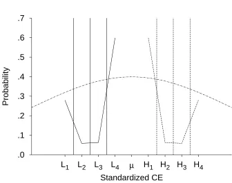
For each prospect, options were either all lower in value than the mean free choice CE (given by another group of participants) or all higher, as illustrated in Figure 1. If a participant is not influenced by the set of options, then his or her choice of option should be that nearest to his or her free choice CE. Under this hypothesis, the expected proportion of times each option will be chosen can be calculated by integrating the free choice distribution between appropriate bounds. The key prediction is that the highest option in the low
condition (L4) and the lowest option in the high condition (H1) should be chosen more than half of the time. This prediction holds for any symmetrical distribution of free choice CEs. Alternatively, if participants' responses are solely determined by the set of options presented to them, then the distribution of responses across options should be the same for both the low and the high value range of option CEs.
Method
Participants. Free choice CEs were given by 14 undergraduates from the University of Warwick. Another 16 undergraduates chose CEs from sets of options. All participated for course credit.
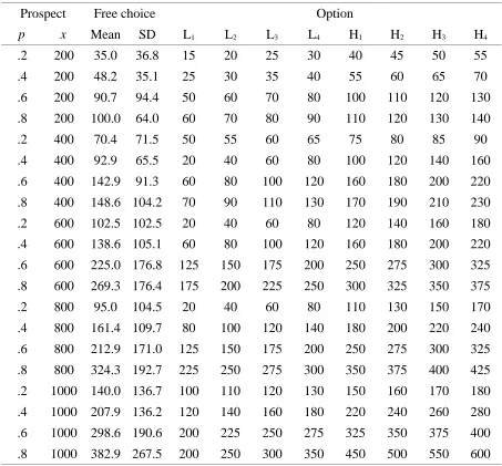
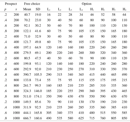
4/6ths of a standard deviation below the mean. In the high options condition, options were 1/6th, 2/6ths, 3/6ths, and 4/6ths of a standard deviation above the mean. Thus the range of each set was half a standard deviation. The spacing of options compared to the distribution of free choice CEs is shown on the abscissa in Figure 1. Options were rounded to have familiar, easy-to-deal-with values.
Procedure. Participants were asked to imagine choosing between £30 for certain or a 50% chance of £100 to illustrate that prospects could have a value. They were told they would be asked to value a series of prospects. It was explained that the purpose of the experiment was to investigate how much they thought the prospects were worth, and that there was no correct answer. Participants were asked to choose the option nearest the value they thought the prospect was worth to them.
Each prospect was presented on a separate page of a 20 page booklet. The ordering of the prospects was random and different for each participant. Probabilities were always presented as percentages. Options were always presented in numerical order, as in the following example of a low option set:
How much is the gamble "60% chance of £400"
worth?
Is it: £60 £80 £100 £120 Results
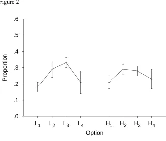
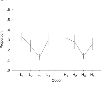
The proportion of times each option was chosen is plotted in Figure 2. There is no evidence that the lowest option in the high options condition (H1) and the highest option in the low condition (L4) were preferred. Instead, the distribution of options is approximately the same for the two conditions. L4 was chosen significantly less than half the time t(7)=4.21, p=.0040. The same was true of H1, t(7)=5.26, p=.0012. An alpha level of .05 was used for all statistical tests.
Discussion
CE judgments were strongly influenced by the CE options offered, and were not skewed towards the mean free choice CE. This data therefore appears to illustrate prospect relativity: People do not seem to form a stable absolute judgment of the value of a prospect, but choose a CE relative to the CEs available. The preference for central options in these data may be an example of extremeness aversion (also called the compromise effect; see
Simonson & Tversky, 1992). Indeed, in choosing amongst identical options, there is a tendency to prefer central ones (Christenfeld, 1995).
Experiment 1B
replicated. Method
Participants. Free choice CEs were given by 35 volunteers. Twenty-eight different volunteers chose CEs from sets of options. All participants were undergraduates from the University of Warwick and none had participated in Experiments 1A. They were paid £5 for taking part in this and other related experiments.
Design and Procedure. The design was the same as in Experiment 1, except that for each participant, 10 trials were randomly selected to have options all higher than the pretest mean for that prospect, the other 10 having options all below the mean. Trials were randomly intermixed. Free choice CEs and corresponding options are given in the Appendix. The procedure was as in Experiment 1A.
Results
Participants took approximately five minutes to complete the task. One participant's data were excluded from the analysis because he had been given a misleading answer to a query about the task which would have led to an inappropriate response strategy. As before, under free choice, the CE increased approximately linearly with both the amount that could be won and the probability of winning.
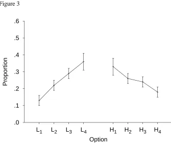
Figure 3 shows the proportion of choices of each option. In both conditions, the proportion of responses increases with proximity to the mean free choice CE. If participants were not affected by the available options, the proportion of L4 and H1 would be expected to be at least .5. Planned t-tests showed that the proportion of L4 and H1 responses was
significantly below 0.5, with values of t(26)=2.65, p=.0135, and t(26)=3.81, p=.0008, respectively.
one point for each time he or she chose the lowest option, two for the next lowest, three for the second highest and four for the highest. Those showing no effect of the option set should have chosen the L4 and H1. However, those who based their judgment entirely on the option set would choose mid-range options. Thus a negative correlation between low choice CEs and high choice CEs would be evidence that people vary in the extent to which context effects influence their CE decisions. Far from being negatively correlated, the scatter plot has a significant positive correlation (r2=.45, p=.0001).
Perhaps surprisingly, we found no evidence that the options offered on the previous trial influenced the option selected on the current trial. One might imagine that, say, offering low options on the previous trial might cause a participant, who is trying to be consistent, to select an option lower than they otherwise would on the current trial. However, the rank (as described above) of the option selected within the set did not depend on the previous option set offered (mean rank 2.63, SE 0.11, for prior low options, and mean rank 2.62, SE 0.13, for prior high options), t(26)=0.23, p=.8407.2
Discussion
consistent with their responses to previously completed questions. Such a consistency effect cannot be due to the immediately preceding trial alone, as there was no effect of the
immediately preceding trial. Instead, if this kind of explanation is correct, the skew must be due to some larger window of previous trials.
Whilst the spacing of the options relative to the free choice distribution of CEs was the same in Experiments 1A and 1B, the options were actually more closely spaced in Experiment 1B because participants' free choice CEs were less variable. Thus an alternate account of the difference in the pattern of preferences across the options could be made in terms of the different absolute spacing of the options. For this reason, we replicated Experiments 1A and 1B as conditions of a single experiment, using the spacings from Experiment 1B throughout. The results remained essentially unaltered, and so we do not present them here. An explanation of the different pattern of preferences in Experiments 1A and 1B in terms of using different options can thus be ruled out.
Experiment 1C
The effect of available options in Experiments 1A and 1B appears to create difficulties for EU and related theories as descriptive accounts of decision under risk. But these difficulties may be less pressing if the effects demonstrated thus far arise only because the options presented as CEs are simply too close together, and that participants are roughly indifferent between them. (Although note that this ought to lead to a 'u' shaped preference across the options, rather than an 'n' shape.3
) If this is the case then these effects should disappear when the options are more broadly spaced, and hence people are no longer indifferent between them. In this experiment we investigated the effect of increasing the spacing of the options.
Method
choice standard deviation as in Experiments 1A and B. In the wide condition the spacing between adjacent options was doubled to 1/3th of a free choice standard deviation. In the gap condition, the option spacing was as in the narrow condition, but the mean of the low and the high options was set to equal that of the wide condition. Eighteen participants took part in the gap condition, and 19 each in the narrow and wide conditions.
Results and Discussion
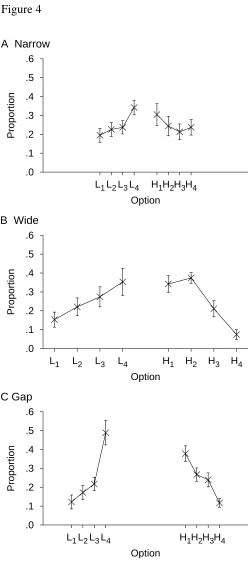
The proportion of times each option was selected is shown in Figure 4. The
proportions for the narrow and wide conditions closely resemble one another. In the narrow condition, option L4 was selected significantly less than half the time, t(18)=4.02, p=.0008, as was the H1 option, t(18)=3.42, p=.0031, replicating the results of Experiment 1B. In the wide condition, option L4 was selected less than half the time, t(18)=2.04, p=.0565, although this difference is only marginally significant. The H1 option was selected significantly less than half of the time, t(18)=3.52, p=.0024. In the gap condition, L4 was not chosen
significantly less than half of the time, t(17)=0.17, p=.8665, but H1 was, t(17)=2.99, p=.0082. For every condition, L4 and H1 were chosen significantly less than the proportion of times predicted by the relevant integrals over the free choice distribution (which was always >.5). The key result is that doubling the spacing of the options did not eliminate the context effect.
Experiment 2
Experiment 2 was designed to demonstrate the same effect of restricting the range of CE options in a task where it was optimal for participants to report CEs truthfully. Although psychologists typically assume that participants are "honest" when providing hypothetical CEs, economists are typically concerned with providing a system of incentives that ensures it is optimal for participants to provide truthful CEs. Hence the results above may be criticized from an economic perspective.
demonstrated preference reversals in choices between two prospects, and CE estimates for those prospects, in situations where decisions were hypothetical and situations where there was an incentive system (see also Tversky, Slovic, & Kahneman, 1990). Preference reversals have also been demonstrated with ordinary gamblers playing for high stakes in Las Vegas (Lichtenstein & Slovic, 1973, see also Grether & Plott, 1979). For further discussion of these and other similar findings see Hertwig and Ortmann (2001) and Luce (2000, pp. 15-16). However, because of the potential importance of the findings from Experiments 1A-C for models of economics, we include this experiment where the incentive system has been designed to motivate participants to provide truthful CEs.
The design follows a solution to the 'cake cutting' problem, where a cake must be divided fairly between two children. One solution is to allow one child to cut the cake into two pieces, and the other child to select the piece. The first child should cut the cake exactly in half, otherwise his or her friend will take the larger piece of cake, leaving him or her with the smaller piece.
In this experiment, participants divide a sum of money into an amount for certain, and an amount that could be be won with a known, fixed probability. For example, they might split £1000 into a sure amount of £300 and the prospect "60% chance of £700". Participants know that the other person (who was not the experimenter) will select either the prospect or the sure amount, taking the better of the two, leaving the participant with the other. Thus it is optimal for participants to split the given amount so that they have no preference between the resulting fixed amount and the resulting prospect. Note that this procedure will work only if each participant assumes that the chooser has the same level of risk preference as himself or herself. To this end, participants were told to assume that the chooser did have the same risk preference as they did.
This procedure more simple than other methods used to elicit truthful CEs, for
In the BDM procedure, participants are given the chance to play a prospect and are asked to state the minimum price at which they would sell the prospect. A buying price is then
randomly generated by the experimenter and, if it exceeds the selling price, then the prospect is bought from the participant. If not, then the participant plays the prospect. It is the case that it is optimal for participants to state a selling price that is the CE of the prospect, though it is unlikely that many participants realize this.
Method
Participants. Participants were undergraduates from the University of Warwick, who had not participated in Experiments 1A-C. Seventeen participants took part in the free choice condition of the experiment. Nineteen further participants took part in the restricted choice conditions. Participants were paid £5, plus performance-related winnings of up to £4.
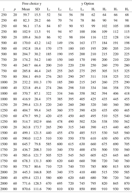
Design. In each trial of the free choice condition, participants divided a given amount of money, x, into two smaller amounts, y and z, to make one fixed amount (y) and the
prospect "p chance of z". Probability p was known to participants before splitting amount x. Participants were told that one trial in the experiment would be selected at random at the end of the experiment and a second person would take either the fixed amount or the prospect for himself leaving the participant with the other option. Under the assumption that the chooser had the same risk preference as they did, it was explained to participants that the chooser would choose the option with greater utility, leaving the participants with their least preferred option, if they did not split the amount to make options of equal utility. It was therefore optimal for participants to split the amount x into amounts y and z, such that y and a "p chance of z" are equivalent for them, i.e., y is the CE for the prospect "p chance of z".
and z values presented might provide them with information about the chooser's risk
preferences. For this reason two people were used in running the experiment. One person was responsible for administering the tests, and the other for making the choice at the end of the experiment. The intention was to keep the roles of the experimenter and the person making the choice at the end of the experiment separate in participants' minds, to minimize the degree to which participants would think that the options provided information about the chooser's risk preference.
It was hypothesized, as in Experiment 1, that the set of pairs of values for y and z presented would influence participants' choices. To investigate this, we varied one between-participants factor. The set of values for y and z were either selected such that y was always greater than the mean free choice value of y and z was smaller than the mean free choice value of z, or vice versa. These correspond to the low and high option sets in Experiment 1. The precise option sets were constructed as follows. The mean and standard deviation of the free choice amount were calculated for each prospect (see Appendix). The two sets of equally spaced options (for the high value and low value conditions) were calculated as described for Experiment 1A. As in Experiment 1A, if participants were not influenced by the set of choices, then the distribution of responses across the options should be biased towards the free choice splitting.
There were 32 trials in the experiment, made by crossing four values of p (.2, .4, .6, and .8) with eight values of x (£250, £500, ..., £2000).
Procedure. All conditions of the experiment began with written instructions. It was explained to participants that they were playing a gambling game, and that they should try to win as much money as possible. They were told that a single trial would be randomly
they thought the amount for certain was equal in worth to a chance on the prospect. Participants were told that if they allocated funds so that either the amount for certain was worth more than the prospect, or vice versa, then the chooser would take the 'better option', leaving them with less than if they had allocated the money so the prospect was worth the certain amount. They were told that although they could not be certain what the chooser would do, they should assume that the chooser would behave like them.
Participants were given five practice trials. One of the trials was chosen at random, and it was explained that if the chooser chose the fixed amount, then the prospect would be played, and they would get the winnings. They were also told that if instead the chooser took the prospect they would get the fixed amount. Note that this discussion was hypothetical, and participants were not actually told what the chooser's preference would be.
After the practice participants completed a booklet of options. The pairs of options were presented in a random order to each participant. An example page from a free choice condition booklet is shown below.
£1000
£____ for certain
or 60% chance of £____
In the restricted choice conditions, pre-split options were presented as in the example below.
£1000
£322 for certain or 60% chance of £678 £334 for certain 60% chance of £666 £346 for certain 60% chance of £654 £358 for certain 60% chance of £642
determine each participant's bonus (using an experiment exchange rate of 0.0024). Results
Participants took between half an hour and one hour to complete the booklet. It seems that the introduction of a bonus caused participants to deliberate on their answers for much longer than in Experiment 1A-C. One participant from the free choice condition was
eliminated from subsequent analysis for showing a completely different pattern of results to other participants, suggesting he had misunderstood the task. The participant had decreased the value of the fixed amount, y, as the chance of the prospect amount, p, increased (i.e., he had responded as if prospects with a higher chance of winning were worth less to him). Fourteen out of 512 trials (16 participants x 32 trials), where the initial amount had been incorrectly split, were deleted and treated as missing data.
For the free choice splits, as the total amount x increased, then participants' allocation of the fixed amount y increased. As the probability p of winning the prospect increased, participants' estimates of the value of the prospect, y, also increased. Thus participants' responses seemed lawful and sensible, indicating that the task made sense to them.
The choices made in the restricted choice conditions are shown in Figure 5. Participants did prefer end options over central options in both conditions, as would be expected if participants were not influenced by the option set. However, if there were no effect of context, L4 and H1 should have been chosen over half of the time. L4 was chosen significantly less than half of the time, t(9)=3.47, p=.0070, as was H1, t(8)=4.20, p=.0023. Thus the proportion of times each option was selected differed significantly from the proportions expected under the assumption that participants were not influenced by the options available.
Discussion
were presented with a range of pre-split total amounts, so that the CE options were either always lower or always higher than the free choice value, the context provided by the pre-split options influenced their choice of CE.
Experiment 3
The demonstration of apparent prospect relativity in risky decision making suggests that the representation of the utility dimension may be similar to that of perceptual
psychological dimensions, where context effects have also been demonstrated. Empirical investigations in absolute identification (Garner, 1953; Holland &
Lockhead, 1968; Hu, 1997; Lacouture, 1997; Lockhead, 1984; Long, 1937; Luce, Nosofsky, Green, & Smith, 1982; Purks, Callahan, Braida, & Durlach, 1980; Staddon, King, &
Lockhead, 1980; Stewart, 2001; Stewart et al., 2002b; Ward & Lockhead, 1970, 1971), magnitude estimation, matching tasks, and relative intensity judgment (e.g., Jesteadt, Luce, & Green, 1977; Lockhead & King, 1983; Stevens, 1975, p. 275) have shown that perceptual judgments of stimuli varying along a single psychological continuum are strongly influenced by the preceding material. If the representation of utility is similar to the representation of these simple perceptual dimensions, then preceding material might be expected to influence current judgments, as it does in the perceptual case.
Simonson and Tversky (1992) provide several cases where preceding material does indeed influence current judgments in decision making. For example, when choosing between pairs of computers that vary in price and amount of memory, the trade-off between the two attributes in the previous choice affects the current choice. Indeed, preference reversals can be obtained by varying the preceding products. In the present experiment we consider the effect of preceding material on judgments concerning a single dimension
Method
Participants. Fourteen undergraduates from the University of Warwick participated for payment of £3. All participants had previously taken part in the free choice condition of Experiment 2.
Design. Participants were asked to state the value of a series of prospects. Participants had previously taken part in a task where estimating the value of prospects truthfully
optimized their reward, compared to overestimating or underestimating the value of a prospect. Participants were instructed to continue providing CEs in the same way.
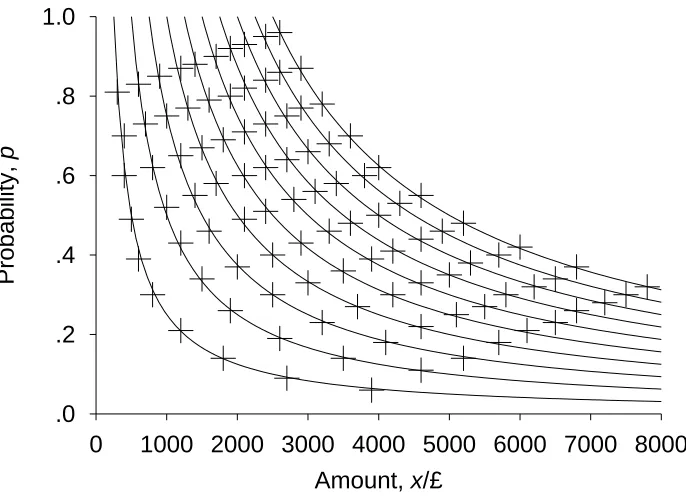
Ten sets of 10 simple prospects of the form "p chance of x" were constructed. Figure 6 shows the values of p and x for each prospect. Each set of prospects lying on the same curve (these are hyperbolas) shares a common expected value. (The slight deviation of the crosses from the line is caused by rounding the values of p and x.) Prospects were chosen in this fashion simply because it produces an equal number of prospects with each expected value. The order in which prospects were presented was random, and different, for each participant.
We hypothesized that the preceding prospect should affect the value assigned to the current prospect as follows. If the previous prospect had a low expected value, then we expected that the current prospect would be overvalued. Conversely, if the previous prospect had a high expected value, then we expected that the current prospect would be undervalued. This prediction is motivated by the contrast effects observed in the analogous perceptual task, magnitude estimation.
Procedure. Participants were told that they would be asked to value prospects, and that they should do this in the same way as in the previous experiment (the free choice condition of Experiment 2). Participants completed a booklet with a separate prospect on each page, together with a space for their valuation.
Results
previous prospect, for each possible expected value of the current prospect. CEs given to a prospect increased as the expected value of the prospect increased. The response was, on average, 97% of the expected value (s.d. 36%) showing slight risk aversion, on average. The expected value of the previous prospect has no effect on the value assigned to the current prospect (i.e., the lines in Figure 7 are flat).
To examine possible sequence effects more closely, a linear regression was completed for each participant, to see what proportion of the variability in the current response could be explained by the previous prospect's expected value, after the effects of the attributes of the current prospect had been partialled out. The previous prospect's expected value was a significant predictor of the current response for just 1 of the 14 participants, no more than would be expected by chance. For this participant, r2
=.04, and for all other participants r2
<.04. Similar analyses for the previous (a) response, (b) x and (c) p also showed no sequential dependencies.
Discussion
In perceptual tasks where a series of stimuli are presented, and a judgment is made after each stimulus, the response to the current stimulus is shown to depend on the stimuli (or responses; the two are normally highly correlated) on previous trials. In other words, the response on the current trial is systematically biased by (some aspect of) the previous trial. Some authors (e.g., Birnbaum, 1992) have suggested that judgments about risky prospects might be similarly affected. Here, CE judgments for simple prospects do not show sequential dependencies like those shown in the analogous perceptual judgment tasks. There is little carry-over of information from one trial to the next. This finding is consistent with Mellers et al.'s (1992) result, where the buying prices of a set of critical prospects were at most only slightly influenced by the expected value of (previously encountered) filler prospects.
Experiment 4
discussion by Luce (2000) highlights the difference between judged CEs, where participants provide a single judgment of the value of a prospect, and choice CEs, derived from a series of choices between risky prospects and fixed amounts. For example, for the kinds of prospects used here, with large amounts and moderate probabilities, judged CEs are larger than choice CEs (e.g., Bostic, Herrnstein & Luce, 1990). The preference reversal phenomenon (e.g., Lichtenstein & Slovic, 1971) is evidence that there is often a discrepancy between choice-based and CE-choice-based methods of assessing utility (see also Tversky, Sattath, and Slovic, 1988). Indeed, Luce (2000) goes as far as to advocate developing separate theories for judged and choice CEs.
Experiment 4 investigates context effects in a choice-based procedure rather than a judged CE-based procedure. Participants make a single choice from a set of simple prospects of the form "p chance of x" where the probability of winning was traded off against the amount that could be won. The context is provided by manipulating the range of values of p (and therefore of x) offered.
Method
Participants. Ninety-one undergraduates from the University of Warwick took part. None had previously participated in any other experiment described in this paper. Payment was determined by playing the prospect selected by each participant, and winnings were between £0 and £2.
Design. Participants were each offered a set of simple prospects of the form "p chance of x". Within the set, the probability of winning and the win amount were traded off against one another, and thus the choice was between a large probability of winning a small amount through to a smaller probability of winning a larger amount. Ten prospects were used: "50% chance of £50", "55% chance of £45", ..., "95% chance of £5".
calculated.4
Figure 8 plots utility as a function of the probability of winning p for different curvatures of the utility function (values of γ). For a risk-neutral person (γ=1.0), for whom utility is proportional to monetary value, the probability of winning for the prospect with the maximum utility is p=.5. For a risk-averse person (γ<1.0), the prospect with maximum utility has a larger probability of winning a smaller amount; the maximum falls at higher p for lower
γ. The key observation is that the prospect with maximum utility in the set is determined by
the level of risk aversion, γ. Thus a participant's choice of prospect can be mapped directly onto a degree of risk aversion.
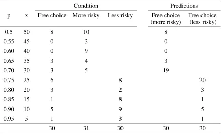
There were three conditions in the experiment. In the free choice condition, all 10 prospects were presented. In two other conditions, the choice of prospects was limited to either the first or second half of the prospects available in the free choice condition. In the more risky condition, the prospects ranged from a "50% chance of £50" to a "70% chance of £30". In the less risky condition, the prospects ranged from a "75% chance of £25" to a "95% chance of £5".
Procedure. Each participant was presented with a sheet listing a set of prospects. The prospects were presented in an ordered table, with a row for each prospect and columns headed "chance of winning" and "amount to win". Probabilities were presented as percentages. Participants were asked to choose one prospect from the set to play. Before making their choice they were given an explanation of how the prospect would be played. The selected prospect was played and participants were paid according to its outcome, multiplied by an experiment exchange rate (0.002).
Results
condition. Two hypotheses were tested. The first is that participants are sensitive to the absolute values of prospect attributes, and are unaffected by the choice options. According to this hypothesis, in the restricted choice conditions, participants should choose the prospect in the set that is nearest to the prospect they would choose under free choice conditions. It is possible to predict the distribution of participants across prospects in the restricted choice conditions from the free choice condition. The last two columns of Table 1 show the distribution of participants that would be expected if the participants in the free choice condition had instead been offered the prospects in one of the restricted conditions. These distributions were generated by summing the frequencies for the prospects in the free choice condition that were unavailable in the restricted choice condition, and adding the resulting count to that for the closest available prospect. The distribution of the more risky condition differs significantly to that predicted from the free choice condition, χ2
(4)=71.82, p<.0001. The distribution of choices in the less risky condition also differs significantly from that predicted from the free choice condition, χ2
(4)=24.55, p<.0001. In conclusion, we can reject the hypothesis that participants in the restricted choice conditions chose the prospect in the set nearest to the prospect they would have chosen under free choice conditions and were otherwise uninfluenced by the set of options.
choices made in each of the restricted choice conditions. Discussion
Participants were asked to select a single prospect to play from a set. Within the set, the probability of winning a prospect was reduced as the amount that could be won was increased. Thus each participant faced a choice between prospects offering small amounts with high probability through to larger amounts with a lower probability. In the restricted conditions, participants were only offered a subset of the prospects available. If participants' preferences were not affected by the set of options provided, they should simply choose the prospect closest to the prospect they would select under free choice conditions. However, the distribution of choices differed significantly from those expected under this prediction. Instead, the set of options available seemed to determine participants' preferences and there was no significant evidence that participants were sensitive to the absolute level of risk implicit in a prospect. In conclusion, the level of risk aversion shown by a participant was shown here to be a function of the set of prospects offered.
However, it is not immediately obvious how the notion of trade-off contrast might account for the results of Experiment 5. Across both contexts the trade-off between
probability and amount was constant (as the chance of winning the prospect was increased by 5%, the amount to win fell by £5). Instead, it seems that participants have no absolute grip of the level of risk implicit in each prospect in the choice set, and instead choose a prospect with reference to its riskiness relative to the other prospects in the set. This demonstration of prospect relativity in choice is consistent with that described in earlier experiments, where CE judgments were used.
Experiment 5
Our final experiment was designed to investigate the extent to which a choice between two prospects is affected by preceding context. Thus this experiment mirrors Experiment 3, but with actual choices rather than CE judgments. On each trial, participants chose between a sure amount of money and a prospect offering a larger amount with a known probability. Let us informally call a trial risky (or safe) to the degree that we expect
participants to prefer the risky prospect (or the sure amount of money). Half of the trials, the common trials, were given to all participants and were designed so that the sure amount was such that a typical, moderately risk-averse participant would be indifferent between the sure amount and the risky prospect. The other half of the trials were filler trials and their
seem relatively safe if the filler trials are “risky”, and participants should favor the safe, sure amount. Conversely, if the filler trials are “safe” then the common trials should seem
relatively risky, and participants should favor the risky prospect. Method
Participants. Thirty-five undergraduates from the University of Warwick took part in the experiment, and were paid £5 for participating in this and three other related experiments.
Design. Thirty-six trials were generated, each of which comprised a simple prospect of the form "p chance of x" and an amount offered for certain. The amounts £100, £200, £300, £400, £500, and £600 were crossed with the win probabilities of .1, .2, .4, .6, .8, and .9 to give 36 prospects. Half of the trials were selected at random and consistently used to set the context. For half of the participants, the fixed amount offered on these trials was low and, for the other half of the participants, the fixed amount was high. The other half of the trials was common to both groups, and the fixed amounts were at an intermediate level.
A sure amount was generated by using Equation 2.
y=x p 1
for each probability, and only once for each prospect amount. Otherwise, the assignment was random and the same for all participants.
Procedure. Participants were given brief oral instructions. They were told that they would have to imagine making choices between playing a prospect to receive an amount of money and taking a smaller amount for sure. Each pair of options was presented on a separate page of a 36-page booklet, and appeared as follows:
Which option do you prefer? 10% chance of £300
£12
Participants were told to mark the option they would prefer and move on to the next page. They were also made aware that there was no objective 'right' answer, and that it was a matter of personal preference.
Results
The dependent measure was the mean proportion of trials on which the prospect was preferred to the sure amount. With “safe” fillers, participants selected the risky prospect significantly more often in the experimental trials (mean .53, SE .04) than in the filler trials (mean .40, SE .05) as intended, t(16)=7.10, p<.0001. With “risky” fillers, participants
selected the risky prospect less often in the experimental trials (mean .47, SE .05) than in the filler trials (mean .67, SE .04), again, as intended, t(17)=7.39, p<.0001. The comparison of interest is performance on the common trials across the “safe” and “risky” conditions. For the common trials the risky prospect was selected slightly more often in the condition in which it was designed to look more attractive, but the difference was not significant t(33)=0.8,
p=.4305. Discussion
sure amount on this trial might seem quite appealing. Conversely, if in previous trials, the sure amount was high compared to the prospect, then the prospect on this trial might seem quite appealing. However, this experiment found no evidence that the properties of preceding trials affected people's judgments between a prospect and a certain amount. The results of this experiment point further to the notion that context effects are much more potent within a trial than between trials, and that this is the case for CE judgments (Experiment 3) and choice paradigms (Experiment 5).
We are quite surprised by the small or lacking effect of previously considered prospects on the current choice, and so have conducted a meta-analysis of sequential effects in other choice experiments from our laboratory. The experiments involved making choices between two prospects, each of the form “p chance of x otherwise y”, where x>y 0. In each pair, one prospect was always more risky than the other (i.e., the probability of winning was smaller) but had a higher expected value. Thus the choice was always between a
comparatively more likely but smaller amount verses a larger but less likely amount. Trials were split into two groups according to whether the total expected value of the prospects on the previous trial was more or less than the median amount. The proportion of risky picks on the current trial did differ significantly between the two groups, t(95)=1.99, p=.0422,
although the actual difference in proportions was very small (.39 when the previous expected value was high, vs. .41 when the previous expected value was low). It seems that this small effect was largely caused by the prospect with the smaller expected value on the previous trial, as a median split of current trials on this attribute lead to a slightly larger significant difference (.39 vs. .42), t(95)=1.99, p=.0079. Splitting by other attributes of the previous trial (e.g., the difference in expected value, the maximum outcome, the higher expected value, the maximum probability of a zero outcome, and the probability of the maximum outcome) does not produce significant differences. In conclusion, it seems that the effects of previous
effects.
General Discussion
Together, the results presented in this paper suggest that prospects are judged relative to accompanying prospects, a phenomenon that we call prospect relativity. In Experiments 1A-C, the set of options offered as potential CEs for simple prospects was shown to have a large effect on the CE selected. In Experiment 2, this effect was replicated despite monetary incentives designed to encourage participants to deliver accurate and truthful CEs. In
Experiment 4, the set from which a simple prospect was selected was shown to have a large effect on the prospect that was chosen. In two further experiments, Experiments 3 and 5, we investigated whether attributes of previously considered prospects affected judgments about a current prospect. Previously considered prospects had little effect. It seems that the context provided by items that are considered simultaneously (e.g., the potential CEs in Experiment 1A-C or the set of available prospects in Experiment 4) does affect decisions about risky choice, but that the context provided by previously considered risky choices, even if they are very recent, has little effect. We call this effect the simultaneous consideration effect.
In the following section we briefly review existing theories of decision under risk, and investigate what account they might offer, if any, of the prospect relativity phenomena
presented. Existing theories can, roughly, be divided into two classes: (a) those where the utility or value of a prospect depends only on the attributes of the prospect, and (b) those where prospect attributes are compared against those of other competing prospects. Independent Prospect Evaluation Theories
the results presented in Experiments 1 and 2. Under EU theory, the utility of a prospect is independent of the other prospects in the choice set. Thus EU theory cannot predict an effect of the context provided by the choice options demonstrated in Experiment 4.
Rank Dependent Utility Theory. In rank dependent utility (RDU) theory (Quiggin, 1982, 1993; see Diecidue & Wakker, 2001 for an intuitive introduction), the independence axiom of EU theory has been relaxed. Instead of transforming probabilities into decision weights, cumulative probabilities are transformed. Thus a decision weight depends not only on the probability of the corresponding outcome, but also on the probabilities of other possible outcomes in the same prospect, modulated by the rank of their associated outcomes. For extreme outcomes such a function causes low probabilities to be over-weighted, and high probabilities to be under-weighted.5
However, for events with intermediate outcomes, the probabilities are minimally distorted (Quiggin, 1993, p. 56). However, as in EU theory, the utility of a prospect is independent of other prospects or options on offer, and thus RDU theory cannot account for these prospect relativity effects.
Configural Weight Models. Birnbaum, Patton, and Lott (1999) describe two
configural weight models, where the utility of a prospect is modified by the rank or difference between the possible outcomes. However, the utility of a given prospect is independent of the other prospects in the choice set, and so these theories cannot account for these prospect relativity effects.
outcomes are gains, as was the case in these experiments, the value of a simple prospect "p chance of x" is given by π(p)v(x), where v is the subjective value function and π is the decision weight function.6
Thus, at least for the simple prospects used in the present
experiments, the value of a prospect is independent of other prospects or options presented, as is the case for EU theory. Thus prospect theory cannot offer an account of these data. Tversky and Kahneman (1992) proposed a modification to prospect theory, where cumulative
probabilities, rather than simple probabilities, are transformed, as in RDU theory. However, this modification does not change the fact that prospect values are independent of other prospects or options in the choice set.
Dependent Prospect Evaluation Theories
In the following theories, the utility or value of a prospect is not independent of the other prospects in the choice set. Thus these theories are potential candidates in accounting for the findings in this paper.
choosing the option in a pairwise comparison with the best option, as this means that dominated options (which presumably would never have been chosen) are ignored. Effectively, regret theory weights states where there is a large difference in (choiceless) utility between choices more heavily.
For the simple gamble “p chance of x”, the CE is such that the difference in utilities between the outcomes, plus the difference in regret, summed over all world states, is zero. As in the independent theories, the options on offer simply do not enter into the equation, and thus regret theory cannot offer an account of the results from Experiments 1 and 2.
In Experiment 4, the set of prospects from which a prospect was to be chosen influenced the choice. As, in regret theory, the utility of a prospect is not independent of the other prospects in the choice set, at first sight it seems that regret theory might be able to offer an account of this context effect. Unfortunately, with 10 independent binary prospects (as in the free choice conditions) there are 210=1024 possible world states, each with a different pattern of possible outcomes depending on which prospect is chosen. Thus it is not obvious what the predictions of regret theory would be. We therefore simulated the results of Experiment 4, assuming utility to be a power function of money, and regret a power function of the difference in the actual outcome and the best outcome that could have occurred (cf. Quiggin, 1994). The key question is, for an individual with fixed utility and regret functions, can regret theory ever predict that, in each set, a non-extreme prospect will be preferred? For every point in the parameter space, if regret theory predicts a mid-set prospect is preferred in one restricted set, then in the other set the corresponding extreme prospect is preferred. Roughly, the pattern of preference for a restricted choice set can always be predicted from the pattern of reference across a free choice of all 10 prospects. In summary, at least for this implementation of regret theory, the context effects in Experiment 4 cannot be predicted.
that subjective prospect attributes are the actual prospect attributes, and the function
comparing attributes gives the difference between them as a proportion of the larger attribute. (No other instantiations of the theory have been investigated.) This proportional difference strategy is a special case of the stochastic difference model, and we apply it to our data. The differences are summed over all attributes to give the overall preference for one prospect over another. This model can account for violations of stochastic dominance, independence, and stochastic transitivity, and thus seems a plausible candidate model to account for the context effects presented in this paper.
The stochastic difference model is primarily a model of choice. It is not obvious how it might be extended to produce CEs. Here, we assume that the CE is a prospect of the form “y for certain” where the model predicts no preference for the CE over the prospect “p chance of x” under consideration. There will be no preference for the prospect over the CE when the proportion difference in the probabilities is equal to the proportion difference in amounts. Thus the model predicts risk neutrality, where the CE is the expected value of the prospect. Allowing the options presented to enter into the evaluation of the monetary attributes as implicit standards (following González-Vallejo, 2002, p. 139) makes no difference, as all of the options are smaller than the amount that could be won.
Preliminary suggestions are given (González-Vallejo, 2002, p. 152) as to how the model might be extended to choice amongst multiple prospects using the notion of trade-off contrast (Simonson & Tversky, 1992) in a two-step procedure. First, the strengths of
preference for one prospect over another are calculated for all pairwise comparisons within the set of prospects. The overall preference for a given prospect is then the sum of all of the pairwise strengths where that prospect was favored. The extended model can be applied to our Experiment 4 as follows.
The stochastic difference model predicts that, for any pair of prospects from
favored. This is because the proportional difference in probabilities is smaller than the proportional difference in money for all pairwise combinations of prospects. Averaging across all pairwise combinations in the free choice condition, the model predicts a skew in preferences towards the more risky prospects, with a "60% chance of £40" most preferred. In the restricted choice conditions, the skew remains, with the most risky prospect being
preferred most in each case. These predictions are independent of the decision threshold (which modulates the weight placed on each attribute). However, given the closeness of the overall preference values, we think that it is unlikely that this prediction is independent of the form of the functions mapping actual attribute values into subjective values or the choice of generalization to the multiple prospect case. Thus we conjecture that the stochastic difference model may be flexible enough to accommodate our data.
Multialternative Decision Field Theory. Roe, Busemeyer, and Townsend (2001) extended decision field theory (Busemeyer & Townsend, 1993) to scenarios with multiple alternatives to offer an account of three key results. Consider a binary choice between two options, A and B, that vary on two dimensions, where one option might be higher on one dimension and the other option higher on the other dimension. In the similarity effect (e.g., Tversky, 1972), the addition of a new competitive option that is highly similar to option A, but not option B, can reverse a preference for A in the binary case to a preference for B in the ternary case. The attraction effect (e.g., Huber, Payne, & Puto, 1982) describes the increase in preference for a dominating option, A, when an asymmetrically dominated option is added to the binary set. In the compromise effect (e.g., Simonson, 1989), an option that represents a compromise between two alternatives (A and B) may be preferred over the alternatives in the ternary choice, even though it was not preferred in either pairwise binary choice.
produce what Roe, Busemeyer, and Townsend (2001) term momentary “valences” for each option. The relative weight for each dimension is assumed to vary over time. Preferences are constructed for each option by integrating valences over time. This process contrasts with the accumulation of absolute attribute values. Instead, valences represent the "comparative affective evaluations" (Roe, Busemeyer, & Townsend, 2001, p. 387). Thus, the choice between options is made in relative rather than absolute terms, as in the stochastic difference model. The second key mechanism is the competition of valences via lateral inhibitory connections such that preferences for more similar options compete more.
There are two natural representations of the simple prospects used in Experiment 4.7 First, the probability of winning and the amount to win can be considered as separate
attributes for each prospect. In this case, the valences for the less risky set (when attending to either the win amount or the win probability) are the same as those for the more risky set. This is because it is the location of the prospects in the space relative to one another that determines their associated valences, rather than their absolute location. Thus multialternative decision field theory predicts that the pattern of preferences should be the same across the less risky and more risky conditions. In other words, the theory predicts pure context effects. Multialternative decision field theory also predicts a tendency to prefer the central prospects in a set in the same way that it predicts the compromise effect.
average subjective EU for all remaining prospects. Thus within a given context, the pattern of valences is the same as the pattern of actual subjective EUs. Thus in the same way that EU cannot predict any context effects, neither can multialternative decision field theory using this second representation.
The Componential-Context Model. Tversky and Simonson (1993) present a model of context dependent preference, which is a generalization of the contingent weighting model (Tversky, Sattath, & Slovic, 1988). The model was devised to provide an account of trade-off contrast and extremeness aversion (Simonson & Tversky, 1992). Each attribute on an object has a subjective value depending on its magnitude. The value of an option is a weighted sum of its attribute values. The value of an option depends on the background context established over previous choices and the current choice set. The effect of the background context is to modify the weighting of each attribute according to the trade-off between attributes implicit in the background context. The value of an option is then modified by the relative value of the option averaged over pairwise comparisons with the other options in the choice set.
Tversky and Simonson (1993) did not apply their model to choices between risky prospects. We consider the representation where probability is simply represented as any other option attribute, as we did for multialternative decision field theory. The effects of choice set in Experiment 4 can then be accounted for as another example of extremeness aversion. Specifically, the componential-context model explains the pattern by assuming that losses on the value of one attribute loom larger than gains in the value of another attribute as the two attributes are traded-off, and thus a central compromise option, where the overall loss is minimized, is preferred. An alternative representation, with a single dimension for the outcome, and probabilities determining the weighting of that outcome, reduces to something like regret theory, and therefore we do not consider it further.
given to an attribute is a function of its position within the overall range of attributes, and its rank. Thus attributes are judged purely in relation to one another. Increasing all of the attributes by a constant value, for example, would not change their position within the range or their rank, and thus, according to range frequency theory, their subjective value should remain unaltered.
There is some precedent for using range frequency theory to account for context effects in decision under risk. Birnbaum (1992) found his data to be consistent with the theory. Recall that he investigated the effect of skewing the values of options offered as CEs for simple prospects. The subjective value of a given option will be larger in the positive skew condition since the option will have a higher rank because of the presence of many smaller options. This is consistent with the finding that, when options were positively skewed, prospects were assigned smaller CEs compared to the case where options were negatively skewed.
individual following such a strategy will display pure context effects. Summary of Theoretical Accounts
Theories where prospects are valued independently of one another, such as EU theory, prospect theory, configural weight theory, and RDU theory, must, by definition, fail to
predict context effects of the sort reported here. When prospects are judged in relation to one another, as in the stochastic difference model, multialternative decision field theory, and range frequency theory, the effect of choice set can, under some circumstances, be predicted. These relational theories all have in common the idea that preferences are constructed for a given choice set (see Slovic, 1995). Regret theory and the componential-context model can be considered a hybrid theories, where utilities derived independently for each prospect are modified depending on their relationship to other prospects in the choice set.
There are two ways in which to view the challenge to theories of decision under risk that cannot explain the prospect relativity effects shown in this paper. First, assume that the theory is correctly representing the underlying decision process and that the context effects demonstrated here merely represent a biasing of judgments. We discuss this possibility below. However, if people are subject to such biases in making everyday decisions, and we see no reason why they shouldn't be, then the descriptive theories should be revised to provide an account of these effects (see Tversky & Simonson, 1993, for a similar point). Given the large size of the effects, there is a second possibility that should be given some consideration; that the models are inadequate, and should be rejected. It is too early to say which of these possibilities is correct. Hybrid models where an underlying EU-type decision process is biased by the context may prove adequate. Alternatively, purely relative models, where judgments about prospects are made relative to the choice set and other anchors, may be extended to account for the classic phenomena that traditional models describe.
Conversational Pragmatics
alternatives on people's choices involves reasoning about the experimenter's intentions. That is, is it critical that participants view the options they are given as provided by a co-operative and reasonable experimenter, and hence infer that their response should naturally fall within that range? If it is, then we might explain the performance that we observe as follows: people have a weak grip on a notion of the utility of a risky option, but they may take the options available as a clue from the experimenter about what answers may be appropriate. They might, for example, assume that the experimenter will have chosen the options so that each will be the choice of some experimental participant. Then, if a participant judges that they are, for example, slightly happier with risk than the average participant, they may decide to choose a value slightly higher than the average option available. Accordingly, context would be expected to play a substantial role in determining participants' choices. This would build connections between the current work and pragmatic theory in linguistic communication (e.g., Grice, 1975; Levinson, 1983).8
hours'. Twice as many respondents claimed to have watched less than 2 1/2 hours of television per night with the latter scale (16% vs. 38%). Schwarz (1994) reports that the effect of response alternatives completely disappears when the informational value of the scale is removed (by saying it is a pretest to explore the adequacy of the response alternatives or by informing the student participants that the scale was taken from a survey of the elderly). Given the similarity of these studies to our experiments, our results may well be attributed to conversational pragmatics.
Anchoring Effects
Alternatively, though, it may be that the set of available options merely 'primes' participants' choices in a way that is insensitive to intentional factors. Tversky & Kahneman (1974) have demonstrated large effects of standard or anchor values in judgment. Estimates are typically assimilated towards the anchor provided, even if participants know that the anchors were randomly selected. Use of randomly selected anchors makes it unlikely that participants take their inclusion to be informative. Further, such effects are evident even for quite implausible anchor values (e.g., Chapman & Johnson, 1994). The more uncertain a participant is about a judgment the more his or her estimates are assimilated towards the anchor value (Jacowitz & Kahneman, 1995). This effect of uncertainty is consistent with a demonstration from Mussweiler and Strack (2000a), who showed that, when the context suggested the category to which an item belonged, anchoring effects were smaller compared to the case where the context did not.
hypothesized to create an anchor-consistent mental model of the target (Mussweiler and Strack, 1999, 2000a; Strack & Mussweiler, 1997). Mussweiler and Strack instantiate this idea in their selective accessibility model by assuming that participants compare a target with an anchor by testing the possibility that the target value is equal to the anchor. This is consistent with the finding that judgments were faster for an implausible anchor, but that subsequent absolute judgments were faster for those participants who had received a plausible anchor. When the anchor is implausible, the judgment can be made without the construction of a mental model of the target. However, when the anchor is plausible a mental model is constructed, causing the judgment to be slower. However, the construction of this model primes the subsequent absolute judgment. For implausible anchors Mussweiler and Strack (2001b) hypothesize that the nearest plausible anchor is considered.
In Experiments 1A-C and Experiment 2, options offered as potential CEs had a large effect on the option chosen. If the options are acting as anchors, then according to
Mussweiler and Strack's selective accessibility model of anchoring, participants test the hypothesis that each option is the CE, and this testing process assimilates the judgment of the CE towards the options. It is less obvious how the selective accessibility model might
account for the choice results in Experiment 4.
One way to test between anchoring and conversational-pragmatic explanations would be to repeat the experiments here, under conditions where participants believe that the ranges of choices are generated randomly (e.g., by spinning a roulette wheel or similar device). Thus, the participants cannot reasonably attribute these choices to a 'co-operative'
experimenter. If the effects described here are intentionally mediated, we would expect the context effects to be eliminated; if they result from non-intentional factors, then they should remain unchanged.
Methodological Implications
theories of decision making under risk and uncertainty. There are various procedures that are typically employed as part of this research, but here we divide them into the two broad categories based on the type of questions they employ. Firstly, there are those procedures that require participants to select between two prospects: choice experiments. Secondly, there are those that elicit a quantity, either probabilistic or monetary, which will cause a participant to be indifferent between two prospects: certainty equivalence experiments. A brief, directional poll of 38 such studies finds that 19 fall into the choice category, 16 are based on certainty equivalence and 3 combine the two.
This paper presents no direct evidence regarding choice experiments involving only two prospects (and we are aware of only a handful of other choice based papers that involve simultaneously presenting more than two prospects). However, we note that Weber and Kirsner (1997) succeeded in manipulating participants into exhibiting greater preference for risky options in an experiment offering choices between two prospects, simply by visually emphasising or de-emphasising the highest outcome relative to the lowest outcome of each prospect. If participants' decisions can be influenced by such a comparatively simple contextual manipulation, then it seems reasonable to speculate that distortions equivalent to those described here might also exist. We therefore conclude that this should be the subject of further research, particularly when considering the relevance to at least half the existing experimental literature.