A Novel Compression Method using Linear
Downsampling and Error Coding
Maria George1, Manju Thomas2
PG Student, Dept. of ECE, College of Engineering Poonjar, Kerala, India1
Assistant Professor, Dept. of ECE, College of Engineering Poonjar, Kerala, India2
ABSTRACT:There are many different downsampling techniques in which most of them are block based methods. In
this compression algorithm, a linear downsampling approach is used. Redundancies in between neighbourhood pixels are reduced using linear downsampler to achieve a part of compression. Error coding is used in many of the image compression techniques. The error signal is the difference between the predicted value and original pixel value. For almost all images, the error histogram has similar properties and a constant set of hop values are derived. Then each error signal is mapped on to set of hop values, which reduces the sum of error value and hop value. The error coder using constant mapping technique reduces the overall algorithm complexity. Downsampler together with error coder achieves the compression. This compression method has simpler processing and also high compression is achieved.
KEYWORDS: Downsampler, Error coder, Hops, PSNR, Prediction, Spatial Domain Image Compression.
I.INTRODUCTION
Image compression is the process of reducing the amount of data for transmission and storage, while preserving the information content in those images. As it is clear, most of the image compression techniques are carried out either before transmission or storage process. And the image reconstruction is carried out at the other receiving end. After the reconstruction process, the image quality is computed to measure the quality and effectiveness of the compression algorithm. These measurements include both subjective and objective analysis. MSE, PSNR, FSIM, SSIM etc are some of such measurements. Based on these results, the image compression techniques are classified in to lossless, near lossless and lossy compression. When the image is reconstructed perfectly, then this is the lossless compression algorithm. If the reconstructed image variation is within a limit, then this will be the near lossless compression. In case of lossy compression algorithms, reconstructed image will only be an approximation of original image and important thing is that a higher compression ratio (lower BPP) can be achieved[3],[4].
In the most of the frequency domain techniques, image is transformed to other domains and a quantization is performed or transform itself compresses the image. During reconstruction, the compressed image is inverse transformed. Quantisation or the transform itself brings the compression. Compression using linear downsampler and error coder has all it’s processing in spatial domain.
There are some techniques which uses the error coding. This algorithm employs the mapping of error signal on to a constant set of values rather than calculating values for mapping each time.
In [1], error coding is used. In this averaging predictor output is given to hops calculator. Using previously predicted pixels a set of hops are calculated and suitable one is selected in such a way to improve reconstruction quality. The negative and positive valued hop indices are present here and this image is downsampled in accordance with some criterion. Two parameters are used to track hop values and is needed to update each time. High compression is achieved using this algorithm.
II.METHODOLOGY
The basic algorithm has two main components: linear downsampler and error coder. Downsampler checks each array of fixed size from the input image to decide whether it is eligible for downsampling. A decision criterion is set to downsample the array. Then the downsampled sequence undergoes linear averaging predictor and corresponding to each predicted value, an error signal is generated. This error signal is mapped using a constant array set (set of hops).The basic block diagram is shown below.
Fig. 1 Block diagram
Input image is given to Redundancy removing block in which the linear downsampler is employed. A given size of array is selected and downsampling decision is made, depending on the threshold set for the difference between the elements in the array. Based on the threshold, the compression ratio and image quality will vary. It is important to note that a trade off occur in between image quality and compression ratio.
Predictor is then employed on downsampled sequence and a linear averaging predictor is used. An error signal sequence is then generated as the difference of predicted signal and original pixel value. The suitable value from the constant set of values called hop array is selected based on the hop selection criterion. It states that the value from the hop array is selected in such a way that it should minimise the sum of error signal and hop value. Only then reconstruction errors will be minimised.
The selection of hop array is of important in the compression. Also the size of hop array will reflect in the image quality and compression ratio. The output of hop selector is that sequence of indices corresponding to the selected hop value. Hence the range of pixel values get reduced .If the hop array size is larger and compression ratio is low, then selected indices values can be further reduced using any reduction methods. Here a simple size reduction is done by allowing some extra single bit for each index value. Then this sequence of indices undergoes coding. The first pixel is transmitted as such to enhance the reconstruction process. Overall compression is achieved through downsampling, hop selection, and coding.
At the reconstruction stage, we have first pixel and sequence of indices. The hop array is same for both encoder and decoder. Using first pixel value we can have prediction for the second pixel. Reconstructed value is the sum of predicted value and hop value corresponding to second pixel. This value is then used for reconstruction of remaining pixels. Each time pixel values are calculated and are further used for reconstruction of next pixel.
III. RESULT AND DISCUSSION
The following experimental results have been obtained by applying the proposed algorithm. Compressor has been tested using two image databases: Kodak lossless true color image suite [3] and USC-SIPI image database [4].
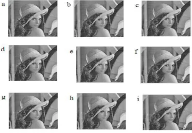
For various threshold values output images of Lena are given in Fig. 2. It is clear that even the image quality is reduced; the variation is not up to expectation regarding the threshold. At higher thresholds, we can have higher compression. Downsampled arrays are reconstructed with same values and it results in thin horizontal bars in reconstruction. It is noticeable only at higher thresholds, since large variations in between pixels are neglected. The no pixels reduced for each array is one less than the array size. Array size variation along with variation of threshold can vary the compression ratio.
Image Redundancy Bit stream
Removing
Block Predictor
Hop Selector
Index
Reduction Coder
Fig. 2 Output image Lena for different thresholds. (a)6 (b)8 (c)10 (d) 18 (e)20 (f) 22 (g)30 (h)40 (i)50
Compression algorithm is tested on other images in database too. Some other input and reconstructed images are given in Fig. 3 and image quality obtained is high. For the hard images, output image quality is higher than that of soft images.
Compression ratio is measured in terms of Huffman coding and arithmetic coding. Both have almost same compression ratio. Elements in hop array are selected such that they are used in compression process with high quality. Also there is an increment of compression ratio in accordance with the increment in threshold. Variations of compression ratio for both methods are given in Fig 4.
Fig. 4 Variation of compression ratio with threshold
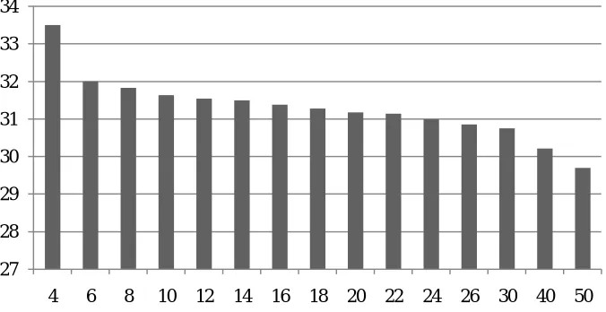
The image quality is preserved for larger threshold; hence a moderate PSNR is obtained for all thresholds. As the threshold value increases, PSNR reduces. This is due to the fact that more duplication of array elements occur at higher thresholds. In figure 5, variation of PSNR as a function of threshold is given.
Fig. 5 Variation of PSNR with variation in threshold
Also the downsampler can’t be applied be applied before coding of indices. This is because even a slight variation in index value at reconstruction will vary image quality drastically. But a lossless downsampling can be attached after hops mapping.
27 28 29 30 31 32 33 34
Fig. 6 No of pixels reduced at pixel redundancy removal.
In Fig 6, no of pixels removed are given as a result of the inter pixel redundancy removing block. Reduction of Pixels has an added advantage of lower processing time. About 180000 pixels can be reduced at a threshold of 50 with moderate image quality and PSNR. This reduction is advantageous for algorithm complexity and processing time. The difference between pixels reduced for a small threshold difference is very high. Linear downsampler also avoids blocking effect in reconstructed image.
IV.CONCLUSION
Compression using downsampler and error coder is a simple efficient algorithm. Predictor, downsampler and the hop selector is of lower complexity. Variation in threshold is associated with variation in compression ratio and image quality. Downsampler doesn’t affect image edges since edges having higher variation in pixel values. Edge preserved downsampling criteria enable to have preserve image features. Linear downsampler has better performance than other methods.
Compression algorithm proposes encoding of the error between pixel predictions and the actual value of it. This encoding is mapped on to a constant set of hops and it has been a simple mapping technique based on hop selection criteria. The constant set is selected once to enhance the algorithm and can be used at both encoder and decoder for any images. The algorithm has to process only the downsampled image and hence processing time is low. Size reduction of selected indices can further improve compression ratio. Downsampler, mapping to hop indices and coding achieves the overall compression.
In future, attaching one or more downsampler ( if it is lossy, it can be added as the pre-processing stage ,else as the down-sampler before coder.) can further improve compression ratio. Sub hop array can be added or adapt to error in hop selection to it as a near lossless compression algorithm.
0 20000 40000 60000 80000 100000 120000 140000 160000 180000 200000
REFERENCES
[1] J J Garca Aranda et al., “Logarithmical hopping encoding: a low computational complexity algorithm for image compression”, IET Image Processing (Volume:9 , Issue: 8 ), July 2015,pp.643 - 651