VICTORIA
~UNIVERSITY
DEPARTMENT OF COMPUTER AND
MA THEMA TI CAL SCIENCES
A Statistical Comparison of Mean and Range Charts with the
Method of Pre-control
PakFai Tang Neil Barnett (34EQRM12) December 1993
TECHNICAL
REPORT
VICTORIA UNIVERSITY OF TECHNOLOGY (P 0 BOX 14428) MELBOURNE MAIL CENTRE
MELBOURNE, VICTORIA, 3000 AUSTRALIA
TELEPHONE (03) 688 4249 I 4492 FACSIMILE (03) 688 4050
A STATISTICAL COMPARISON OF MEAN AND
RANGE CHARTS WITH THE METHOD OF
PRE-CONTROL
PAKFAITANG AND NEILBARNETT
Department of Computer and Mathematical Sciences, Victoria University of Technology, PO Box 14428 MMC, Melbourne, Victoria 3000, Australia.
SUMMARY
This paper provides a rationale for making a statistical comparison between the techniques of 'pre-control' and traditional x and R
charts. Special attention is drawn to the application of both
techniques to the short run manufacturing environment where, for the use of X and R charts, the issue of parameter estimation is an
additional problem. The total discussion is given in the context of the manufacture of discrete items.
KEY WORDS Pre-Control X and R charts Adjusted Limits Statistical Comparison Assumed cp value
INTRODUCTION
In 1924 Dr. Walter Shewhart first introduced the X and R charting
technique for the statistical monitoring and control of industrial processes. Now, after many decades of use, they have become the core around which has been built a body of statistical techniques expressly designed for the purpose of controlling the quality of manufactured products.
A competing procedure, employing a different strategy and known as 'pre-control' (p.c.), was proposed by Shainin 11 in 1954 as
a replacement for various special purpose plans for quality control and, in particular, as an improvement to the then 30 year old
technique of
x
and R control. 'Pre-control' focuses directly onWhen 'weighing' the merits and disadvantages of competing
industrial control procedures, issues such as statistical efficiency,
cost effectiveness, extent and ease of use need all to be considered.
In fact these factors, to varying degrees, play major roles in
determining the overall success of quality monitoring, maintenance
and improvement efforts.
After giving a brief outline of 'pre-control' and re-iterating its
acclaimed practical benefits, this paper provides a rationale for
making a statistical comparison between the technique and that of
traditional x and R charts. It is assumed that the reader is familiar
with the latter. Special attention is drawn to the application of both
techniques to the short run manufacturing environment where, for
the use of X and R charts, the issue of parameter estimation is an
additional problem. The total discussion is given in the context of
the manufacture of discrete items.
A REVIEW OF PRE-CONTROL
The basic principles underlying the 'pre-control' technique are
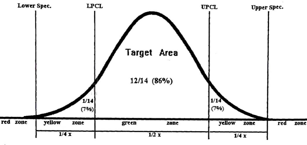
Figure 1. Pre-Control Scheme
Lower Spec. LPCL UPCL Upper spec.
Target Area
12/14 (86°/o)
red zone zone green zone yellow zone
1/4:x 112 x 114 :x
Suppose that the quality characteristic of interest is of the variable
type such as a physical dimension. The tolerance is divided in three
and the boundaries of the middle section called 'pre-control' lines.
The area between these lines is described as the 'target area' or the
green zone. The remaining areas between the specifications are
labelled the yellow zones and those beyond the specification limits
are termed the red zones. If the process is just capable of meeting the specifications, (i.e its cp value is 1) and if centered at the
nominal dimension then, by normal theory, approximately 1in14
times an observation will fall in either yellow zone by chance alone.
It is assumed that the product characteristic under focus follows a
normal distribution with a standard deviation of cr. A single
observation falling in these zones is not deemed an indication of
the presence of a process disruption. Two consecutive values in
these zones, however, or one in the red zone, is considered
adequate evidence of trouble and grounds for process adjustment.
'Pre-control' operating rules are developed around these
fundamental notions. In a modified version, the well known
'first-piece inspection' procedure for approval of set-up and resumption
of a corrected process is substituted with the somewhat tighter rule
' ... If five consecutive units are within the target area before the
occurrence of a red or a yellow, the set-up is qualified and full
production can begin ... ' The reason is, that the occurrence of this
event indicates that the process is well centered and capable of
producing at a satisfactory quality level with a high probability.
The probabilities of approving a set-up which is centered at the nominal dimension, for various process capabilities, Cp, and using
the above rule, are given in Table 1.
Table 1. Probability of Set-up Approval or Pre-Contro 1
cp 0.50 0.75 1.00 1.25 1.33 1.50
Prob. 0.0489 0.2210 0.4882 0.7308 0.7919 0.8838
If five consecutive greens prove difficult to obtain, then this is an
indication that the process is either incorrectly centered and
requires adjustment, or that the process is not capable of
consistently meeting the specifications. This check rule is useful for
short production runs for which the 'set-up' is a crucial factor
affecting the quality of the subsequent process output.
Once the process has passed the initial set-up stage,
periodically 2 consecutively produced items are examined to
monitor performance. Having items in either of the yellow zones is
acceptable, except when two occur consecutively. Two successive ·
yellows on the same side of the target, signal the impending
If they occur on different sides of the target, the process spread has most likely increased beyond its acceptable limit. In this manner,
'pre-control' enables corrective action to be taken before
unacceptable work is produced and, hopefully, avoiding repeated minor, and unnecessary corrections. In the event of getting an item in either part of the red zone, the process is stopped immediately, as it is already producing defective items! Variations in this 'pre-control' plan, applicable to less common situations are given in Shainin 11 and Putnam 8.
In order to justify his recommendation for 'pre-control', Shainin
11,12,13,14 made some efforts to discuss its statistical power. These
included consideration of the long run expected proportion of
nonconforming units produced resulting from the ongoing use of 'pre-control' based on a particular sampling rule. He showed that the
maximum value of this quality measure, termed the average produced quality limit (APQL), does not exceed 2o/o for normally distributed processes if 6 inspection checks, on average, are made between typical process adjustments, 13. Some very general discussion about the
sampling frequency appeared in Satterthwaite 9, Shainin 15 and Traver
17. Without previous knowledge of the average time between process
adjustments, Shainin 14 suggested that a 20-minute sampling interval
should first be used and adjusted subsequently.
As pointed out in 4, some of the expressed doubts about
'pre-control' relate to the normality assumption. In this regard, Shainin 15
stated that the effect of the process distribution is not significant to 'pre-control' as the method assists in controlling the manufacture of defects ... 'by the size of the yellow zones, but not by the target area' ! Sinibaldi
16 used simulation techniques to examine the effect of non-normality on
relative performance of 'pre-control' and
x
and R control on normal andskewed distributed processes with frequently changing means. The
results of the comparison indicate that x control causes less incorrect
mean shift signals and has better control to target ( as measured by the
overall average, x and the average distance of all items produced from
the process target) than 'pre-control'. However, using the R chart to
detect deterioration in the process spread results in more false alarms
than using 'pre-control' for the same purpose.
Bhote 2 attempted to illustrate some 'weaknesses' in X and R
control charting, using two case studies. Taking a more complete
view, Logothetis s argued effectively that, despite its simplicity,
'pre-control' cannot be considered a serious alternative to SPC. He,
in fact, used the same case studies as Bhote 2 ( who used them to
illustrate the 'weaknesses' of X and R control charts) to
demonstrate the usefulness of SPC as a whole and the weaknesses
of 'pre-control'. However, no comparison has been made between
'pre-control' and
x
and R charts on the basis of average run length(ARL). This is due to the fact that, 'pre-control' lines are derived
from specification limits, causing the ARL for a given mean shift to vary according to the actual process capability ( cp).
THE PRACTICAL MERITS OF PRE-CONTROL
The~e is little mention of 'pre-control' in many standard text books
on statistical process control, despite it having certain practical
advantages over X and R charts. This could indicate a belief that a
reasonable statistical comparison between the two techniques is
since the method has proven useful over many years and in many
industries or indicate a view aligned with that of Logothetis s that
'pre-control' is too limited in its perspective.
With the unique setup rule of 'pre-control', the first five
consecutively manufactured units are all that is required to
determine whether any process-tolerance incompatibilities exist
before full production is allowed to commence. There is, of course,
no definite knowledge of how many units will have to be checked
before five un-interupted good ones are obtained. In comparison,
when using X and R charts, it is necessary to have fairly long
process trial runs in order to collect sufficient sample data to
establish the existence of a state of statistical control, and
subsequently, to estimate .the process standard deviation so as to
correctly locate the control lines.
Following setup approval, 'pre-control' provides for the
occasional sampling of 2 consecutively produced units to monitor
on-going process performance, in contrast to the routine sample
size of 4 or 5 often recommended for
x
and R charts. Nocalculations need to be performed for 'pre-control' operation except
for the extremely simple initial setting of 'pre-control' lines,
whereas continual routine computations are involved with use of
x and R charts. For these latter, it is not only necessary to calculate
the control statistics for subgroups, but also necessary to estimate
and revise the control limits from time to time.
For 'pre-control', measurements can be seen, compared to
specification limits and easily understood by operators without the
likelihood of misunderstanding or misinterpretation. Additional
be gained through operators having a better appreciation of the
techniques in use.
Whilst, in practice, determination of the sampling interval
for x and R charts is arbitrary, 'pre-control' provides a simple and
flexible rule of 6 inspection checks per trouble indication which, on
a long term basis, results in a maximum average fraction defective
of less than 2°/o for a normally distributed process 13. A successful
application of 'pre-control' in a 'zero defects' environment has been
reported by Brown 3Regulating sampling on the basis of recent
process performance, seems a more reasonable and efficient
approach to adopt than sampling at fixed intervals, as it entails
more frequent sampling when the process is unsatisfactory.
Such eventualities as tool wear do not cause a premature
reaction from 'pre-control'. It will only issue warning signals at
times when the process is soon likely to produce defective
products.
Since 'pre-control' does not require exact measurements but
only needs to note the zone into which the measurements fall,
complex and expensive measuring equipment may be replaced by
'go/no-go' colour coded gauges. Furthermore, electronic gauging
can be considerably simplified if it is only required to distinguish
between a few measurement bands. As a result, there can be a
reduction in capital investment and calibration costs.
Another important feature of 'pre-control' is its ready
applicability to a variety of situations including the short
production run manufacturing environment which has become
increasingly common following the general move into Just-In-Time
Despite its many years of existence, however, and its
apparent practical merits, given in brief here, 'pre-control' has not
been widely adopted as a replacement for traditional
x
and Rcharts. Logothetis s extensively criticised adoption of 'pre-control'
over use of X and R charts on a number of grounds. It is intended
that the material contained in this paper will provide some
additional, statistically based material, that will help facilitate a
rational judgement on which of the two techniques to adopt in any
given situation.
SHORT RUNS AND PRE-CONTROL
There is no universally agreed definition of a 'short run', however,
the term is generally used to describe production processes with
typically less than 50 items made within a single machine set-up.
Short runs, therefore, at first glance, do not readily lend themselves
to the use of Shewhart X and R charts.
The essential problem that obstructs the application of
standard control charting techniques in short production run
situations, is the inability to estimate the process variability,
because of insufficient data. The problem is further aggravated by
problems of process 'warm up'. This phenomenon is commonly a
dominant feature in short-run processes, as instability after setup
or reset can represent a large proportion of production time.
Neglecting this fact and using data from such a period to obtain
control limits can lead to erroneous conclusions regarding past,
current and future states of the process. Murray et al. 7
Unlike x and R charts, 'pre-control' is a control technique
which predetermines its control limits by reference to product
specifications only, rather than requiring an accumulation of data
for computation of them. It is also capable of handling the problem
of process 'warm up'. It is, therefore, highly suitable for application
to short production runs.
A STATISTICAL COMPARISON BETWEEN PRE-CONTROL AND
X-BAR AND R CHARTS
For short production runs, when there is insufficient previous data
necessary to obtain the control limits for
x
and R charts, a numberof authors (see, for example, Sealy 10 and Bayer 1) have proposed
setting control limits on the assumption that the process is just .
capable of meeting specifications, and assuming that the mean
level of the process is equal to the nominal specification. This
approach is used here to provide a basis for a statistical comparison
between 'pre-control' and X and R charts.
In the following comparison, a subgroup size of 4 is chosen
for the application of x and R charts because this is commonly
recommended. It is also assumed that the quality characteristic
under consideration is normally distributed and that no
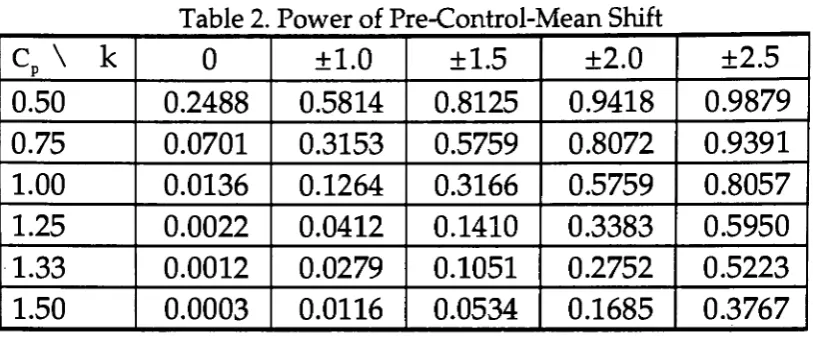
supplementary run rules are used with the x chart. First, consider
the probabilities of detection by the sample immediately following
a process mean shift, using an
x
chart and a 'pre-control' chart.These probabilities are provided in Tables 2 and 3 for various
combinations of process capability (cp) and mean shifts in
multiples (k) of the standard deviation (a). In both tables, the
shift except when k
=
0, in which case the values tabulated are theprobabilities of a false warning. Signals from 'pre-control' that we
employ here as indication of a process mean shift, are 2 consecutive
items in the same yellow zone, or 1 in the red zone and the other
not falling beyond the 'pre-control' line on the opposite side of the
nominal value. Furthermore, it should be noted that the control
limits for the X and R charts are set using conventional control chart
factors with the additional assumptions that,
U+L U-L
µ= and a =
-2 6
The entries in Table 3, other than those corresponding to cp
=
1, arethe probabilities of detecting a mean shift of the indicated
magnitudes when the cp has been assumed to be 1 but is in fact one
of the values indicated. It has been adequately demonstrated in the
literature that the X chart is tardy in registering small changes in
the process mean. Where the 'speedy' detection of small mean
shifts are required, additional control rules or alternative charting
techniques are necessary. Thus the tables provide, for comparison,
probabilities for a number of realistic mean shifts; realistic in the
sense that they reflect situations where x (with no additional rules)
and 'pre-control' can conceivably be considered competing
techniques. Besides having a lower likelihood of a false signal, the
x
chart possesses a higher probability of 'picking up' the mean shift irrespective of the actual process capability, except where indicatedby*, when the differences between corresponding entries in the
two tables are marginal. In one sense, a more reasonable
comparison can be accomplished through adjusting the control
'pre-control'. This involves moving the control lines nearer to the
nominal value. Following such a modification, the corresponding
probabilities of immediate detection are given in Table 4. Tables 2
and 4 clearly illustrate the superiority of the x chart in terms of
sensitivity to process mean shifts.
Table 2. Power of Pre-Control-Mean Shift
cp \ k 0 ±1.0 ±1.5 ±2.0 ±2.5
0.50 0.2488 0.5814 0.8125 0.9418 0.9879
0.75 0.0701 0.3153 0.5759 0.8072 0.9391
1.00 0.0136 0.1264 0.3166 0.5759 0.8057
1.25 0.0022 0.0412 0.1410 0.3383 0.5950
· l.33 0.0012 0.0279 0.1051 0.2752 0.5223
1.50 0.0003 0.0116 0.0534 0.1685 0.3767
Table 3. Power of X-bar Chart with 3cr Limits (assumed Cp = 1)
cp \k 0 ±1.0 ±1.5 ±2.0 ±2.5
0.50 0.1336 0.6915 0.9332 0.9938 0.9998
0.75 0.0244 0.4013 0.7734 0.9599 0.9970
1.00 0.0027 0.1587 0.5000 0.8413 0.9773
1.25 0.0002 0.0401* 0.2266 0.5987 0.8944
1.33 0.0001 0.0232* 0.1611 0.5040 0.8438
1.50 0.0000 0.0062* 0.0668 0.3085 0.6915
Table 4. Power of X-bar Chart with adjusted Limits (assumedCP
=
1)cp \k 0 ±1.0 ±1.5 ±2.0 +2.5
0.50 0.2173 0.7782 0.9613 0.9972 0.9999
0.75 0.0642 0.5594 0.8748 0.9842 0.9992
1.00 0.0136 0.3201 0.7028 0.9373 0.9943
1.25 0.0020 0.1391 0.4664 0.8201 0.9723
1.33 0.0010 0.0985 0.3890 0.7637 0.9571
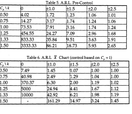
Tables 5 and 6 provide average run-lengths for detection of a
mean shift using 'pre-control' and an x chart respectively, based on
the probabilities contained in Tables 2 and 3.
Table 5. A.R.L Pre-Control
cp \k 0 t±:l.O l±l.5 ±2.0 t±:2.5
0.50 4.02 1.72 1.23 1.06 1.01
0.75 14.27 13.17 1.74 1.24 1.06
1.00 73.53 7.91 ,B.16 1.74 11.24
1.25 1454.55 l24.27 7.09 I 2.96 1.68
1.33 833.33 B5.84 ~.51 3.63 1.91
1.50 13333.33 86.21 18.73 5.93 l2.65 I
Table 6. A.R.L X Chart (control based on Cp
=
1)cp \k '0 t±:l.O C!:l.5 t±2.0 0:2.5
0.50 7.49 1.45 1.07 1.00 1.00
0.75 40.98 ~.49 1.29 1.04 1.00
1.00 370.37 6.30 2.00 1.19 '1.02
1.25 5000 l24.94 4.41 1.67 1.12
1.33 10000 ~2.92 6.21 1.98 'l.19
1.50
-
161.29 14.97 B.24 1.45Of course an ARL comparison is particularly meaningful if it is
assumed that the sampling interval is common for the two
methods. This further raises the matter of sampling effort, since
'pre-control' has an implied sample size of 2 and the x and R charts
being used here for comparison, have a sample size of 4. This
matter will be discussed later.
Tables 7, 8 and 9 are extensions to Table 3. where different cp
values are assumed at the outset. From these it can be seen that if
c,
is taken to be 0.75 then Xis superior only for those casesfor all cases in having smaller probabilities of false alarms. When
cp is assumed to be 1.25, even if the actual value is as low as 0.5 or
as high as 1.50 the x chart is superior for detecting all the given
mean shifts. The probabilities of false alarms for the two methods
are compatible. Similarly for the assumption of cp = 1.50, except
here, 'pre-control' is superior with respect to false alarms.
T bl 7 P a e . owero f X b Ch - ar art assume ( d
c
:p-- 0 75) .c \
p k ' 0 ±1.0 ±1.5 ±2.0 ±2.50.50 0.0455 0.5000 0.8413* 0.9773* 0.9987* 0.75 0.0027 0.1587 0.5000 0.8413* 0.9773* 1.00 0.0001 0.0228 0.1587 I 0.5000 ! 0.8413*
. 1.25 0.0000 0.0014 0.0228 0.1587 0.5000 1.33 0.0000 0.0005 0.0102 I 0.0934 0.3745 1.50 0.0000 0.0000 0.0014 0.0228 0.1587
T a e bl 8 P . owero f X b - ar Ch · art assume ( d
c
· :p= .
125)cp \ k 0 ±1.0 ±1.5 ±2.0 ±2.5
0.50 0.2301 0.7881 0.9641 0.9974 0.9999 0.75 0.0719 0.5793 . 0.8849 0.9861 0.9993 1.00 0.0164 0.3446 0.7258 0.9452 0.9953 1.25 0.0027 0.1587 0.5000 0.8413 0.9773 1.33 0.0014 0.1166 0.4239 0.7905 0.9647 1.50 0.0003 0.0548 0.2743 0.6554 0.9192 1
1
T a e . ower o bl 9 P fX b - ar Ch art assume d (
c
:p-- 150).
cp \ k 0 ±1.0 ±1.5 ±2.0 +2.5
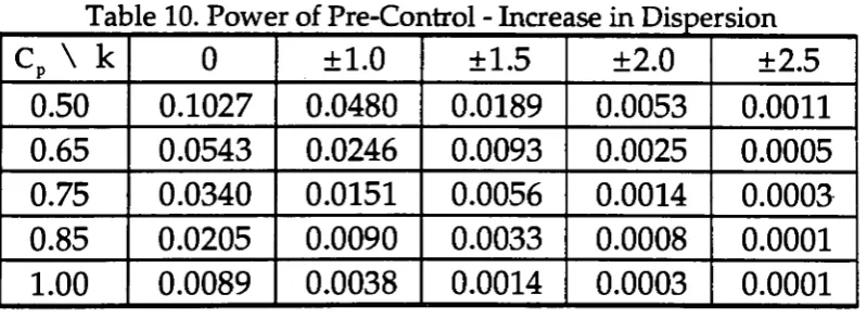
It is also of value to study the probabilistic behaviour of these
two control techniques in relation to how quickly they respond to
an increase in process dispersion. For 'pre-control', 2 successive
measurements beyond different 'pre-control' lines constitute a
warning signal that the process spread is worse than the one
implicitly assumed. However, the occurrence of this event does not
only depend upon the process capability, it is also affected by the
deviation of the process mean from target. As reflected in Table 10,
for a given level of process capability, the larger the deviation, the
smaller the chance of getting such a signal. The corresponding
probabilities of a signal from the R chart are given in Tables 11 and
12 for the cases where conventional and adjusted control limits are
used. Control lines are adjusted in the sense that they equate the
probabilities of false alarms for the two methods. As shown in
these tables, an R chart clearly provides better protection against a
worsening process capability. Tables 13 and 14 show the power of
the conventional R chart when the assumed cp is greater than 1 .
Ta bl e 10. owero p f P C re- ontro -1 In crease m 1spers1on . o·
cp \ k 0 ±1.0 ±1.5 ±2.0 ±2.5
0.50 0.1027 0.0480 0.0189 0.0053 0.0011
0.65 0.0543 0.0246 0.0093 0.0025 0.0005
0.75 0.0340 0.0151 0.0056 0.0014 0.0003
0.85 0.0205 0.0090 0.0033 0.0008 0.0001
1.00 0.0089 0.0038 0.0014 0.0003 0.0001
Table 11. Power of R Chart-Conventional Limits (assumed Cp = 1)
cp 0.50 0.65 0.75 0.85 1.00
T bl 12 P a e owero f RCh art-Ad' l]US t e d L' lffil 't s
cp 0.50 0.65 0.75 0.85 1.00
Prob. 0.3940 0.1715 0.0850 0.0376 0.0089
T a e bl 13 P owero fRCh art ( assume d
c
.p= 125) .cp 0.50 0.65 0.75 0.85 1.00 1.25 Prob. 0.5445 0.3093 0.1904 0.1078 0.0393 0.0049
T a e bl 14 P owero f RCh ar assume t ( d
c
.p= 150) .cp 0.50 0.65 0.75 0.85 1.00 1.25 1.50 Prob. 0.6851 0.4745 0.3445 0.2355 0.1192 0.0289 0.0049
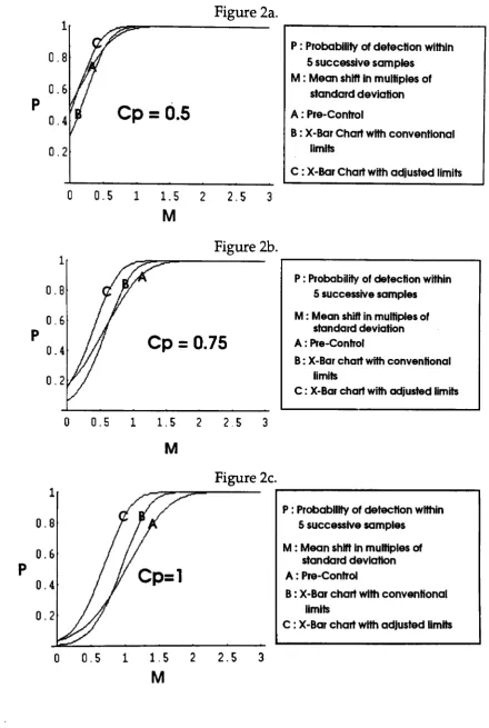
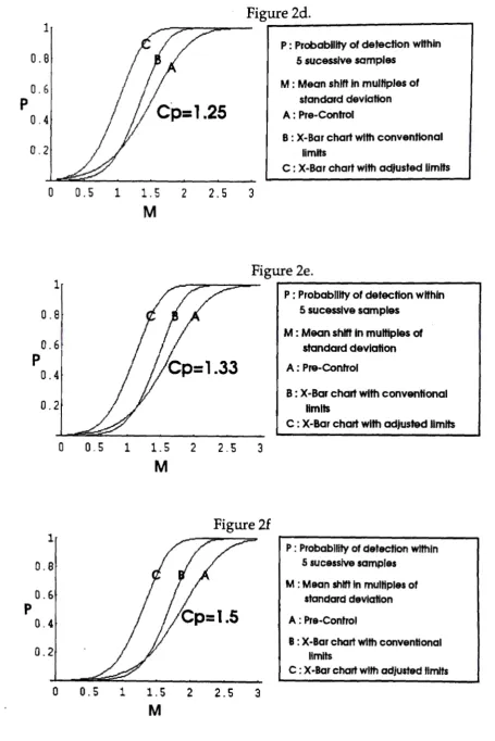
If the x and R charts are for use with short production runs, it may
riot make a great deal of practical sense to compare their effectiveness
with 'pre-control' on the basis of average run length, as was done in
Tables 5 and 6. This is the case when the total production time is less
than the time taken to collect enough samples to match the ARL. As an
alternative, we consider the probability of detection within 5 successive
samples following a given mean shift. This probability is plotted against
process mean shift in standard deviation units for 'pre-control' and
x
charts with both conventional and adjusted control limits in figures 2a
to 2f where the x chart is constructed under the assumption that cp is
1. As shown, there is no remarkable difference between 'pre-control'
and x charts with either conventional or adjusted control limits if
cp =0.5 or 0.75. However, considerable differences exist between these
techniques if the process is more than capable, especially for mean
1
Figure 2a.
0.8
P : Probablllty of detection within 5 successive samples
M : Mean shift In multiples of
0.6 standard deviation
p
Cp
=0.5
A : Pre-Control0.4
B : X-Bar Chart with conventional
0.2 limits
C : X-Bar Chart with adjusted limits
0 0.5 1 1. 5 2 2.5 3
M
Figure 2b. 1
P : Probability of detection within
0.8 5 successive samples
0.6 M : Mean shift in multiples of
standard deviation
p
Cp
=
0.75
A : Pre-Control0.4
B : X-Bar chart with conventional
0.2 limits
C : X-Bar chart with adjusted limits
0 0.5 1 1. 5 2 2.5 3
M
Figure 2c.
1
P : Probability of detection within
0.8 5 successive samples
0.6 M : Mean shift In multiples of standard deviation p
A : Pre-Control
0.4
B : X-Bar chart with conventional
0.2 limits
c: X-Bar chart with adjusted limits
0 0.5 1 1.5 2 2.5 3
1
0.8
0.6
p 0.4
0.2
0
1
0.8
0.6
p 0.4
0.2
0
1
0. 81
0.6 p
0.4
0.2
0
0.5 1
0.5
0.5 1
1
1.5 M
1.5 M
1.5
M
2 2.5
Figure 2d.
3
P : Probability of detection within
5 sucesslve samples
M : Mean shift in multiples of
standard deviation
A : Pre-Control
'
B : X-'Bar chart with conventional limits
c : X-Bar chart with adjusted limits
Figure 2e.
..--...-..,,----==--2 2.5 3
Figure 2f
2 2.5 3
p : Probability of detection within 5 sucesslve samples
M : Mean shift In multiples of
standard deviation
A : Pre-Control
B : X-Bar chart with conventional limits
c : X-Bar chart with adjusted .limits
P: Probability of detection within 5 sucessive samples
M : Mean shift In multiples of standard deviation
A: Pre-Control
B : X-Bar chart with conventional limits
EQUATING SAMPLING EFFORT
In the discussion so far, the total sampling effort hasn't been taken
into consideration; the assumption being made that the time and
cost of sampling, measurement or testing are not significant. This
may, however, be unrealistic in certain circumstances. If it is, no
useful comparison can be made unless the relative sampling
frequency of 'pre-control' and X and R control is first set in such a
way that both methods involve the same sampling effort.
To compensate for the smaller sample size of 2 for
'pre-control', we assume that process checks are made twice as often as
x
and R control with a sample size of 4. This being the case, wefocus on the average number of items required to detect a change
in the process mean or process dispersion, using the two methods.
In Tables 15 and 16, the average number of units sampled
before 'picking up' various mean shifts under different process
capability levels are given for 'pre-control' and
x
chart control (control lines fixed on the basis that cp = 1). To facilitate thecomparison, we have computed the following index :
I ={ANIIMs(PC) if k=O
MS ANll(X)
I = { AN/I ( X) if k -:;; 0
MS ANIIMs(PC)
where
ANllMs(PC) is the average number of items inspected before
detecting the mean shift using 'pre-control' except when k=O, in
which case it is the average number of items inspected prior to the
ANII(X) is the average number of items inspected before detecting
the mean shift using a conventional x chart (control based on
cp =I) except when k=O, in which case it is the average number of
items inspected prior to the occurrence of a false signal.
If IMs > 1whenk'¢0 then 'pre-control' performs better than an
x chart in the sense that, on average, it 'picks up' the mean shift
with fewer sampled items. Similarly, when k = 0 and IMs > 1 then
'pre-control' takes longer, on average, before issuing a false signal.
The values of this index for various combinations of mean shift (in
multiples of cr) and actual process capability are tabulated in Table
17. As shown, whilst being superior in detecting mean shifts of all
the given magnitudes, irrespective of the actual process capability,
'pre-control' is far worse than
x
control with regard to false alarms,a factor alluded to by Logothetis s.
a e LMS
T bl 15 ANTI (PC)
cp \ k 0 ±0.5 ±1.0 ±1.5 ±2.0 ±2.5 ±3.0
0.50 8.04 6.30 3.44 2.46 2.12 2.02 2.00
0.75 28.53 15.95 6.34 3.47 2.48 2.13 2.03
1.00 147.01 56.60 15.83 6.32 3.47 2.48 2.13
1.25 917.36 243.97 48.53 14.19 5.91 3.36 2.45
1.33 1686.06 400.16 71.69 19.03 7.27 3.83 2.63
T bl 16 ANil(X) ( a e samp e size , ontro 1 . 4
c
lb ased on Cp = 1)cp \ k 0 ±0.5 ±1.0 ±1.5 ±2.0 ±2.5 ±3.0
0.50 30 13.0 5.79 4.29 4.03 4.00 4.00
0.75 164 37.9 9.97 5.17 4.17 4.01 4.00
1.00 1481 175.8 25.21 8.00 4.75 4.09 4.00
1.25 22611 1342.4 99.85 17.65 6.68 4.47 4.05
1.33 60458 2867.5 171.71 24.83 7.94 4.74 4.09 1.50 588674 17189.8 644.16 59.87 12.96 5.78 4.29
T a e bl 17 I • :rvf<:;
cp\ k 0 ±0.5 ±1.0 ±1.5 ±2.0 ±2.5 ±3.0
0.50 0.2685 2.0580 1.6815 1.7414 1.8955 1.9763 1.9967 0.75 0.1744 2.3736 1.5717 1.4894 1.6818 1.8838 1.9744 1.00 0.0992 3.1066 1.5931 1.2665 1.3691 1.6490 1.8778 1.25 0.0406 5.5024 2.0575 1.2442 1.1300 1.3305 1.6511 1.33 0.0279 7.1660 2.3952 1.3048 1.0921 1.2382 1.5558 1.50 0.0109 14.3105 3.7290 1.6001 1.0921 1.0896 1.3467
A similar comparison between 'pre-control' and use of the R
chart (control based on cp = 1) with respect to detection of increase
in process variance can also be made. Let
I
=
ANIIvr(PC) if C=
lVI ANII(R) p
Ivr
=
ANII(R) if CP < 1 ANIIvr(PC)where
ANIIvr(PC) is the average number of items inspected before detection of
the increase in process spread using 'pre-control' except when cp = 1, in
which case it is the average number of items inspected prior to the
occurrence of a false signal.
ANII(R) is the average number of items inspected before detection of the
on
cp
= 1) except whencp = 1, in which case it is the average number ofitems inspected prior to the occurrence of a false signal.
The values of ANIIVI(PC), ANII(R) and IV! are provided in Tables 18, 19
and 20 respectively. The R chart can be seen to be more sensitive to
increases in the process spread except where marked by*.
a e .VT1
T bl 18 ANII (PC)
cp \ k 0 ±0.5 ±1.0 I ±1.5 ±2.0 ±2.5 ±3.0
0.50 19.47 23.59 41.70 105.77 375.23 1805.10 11445
0.65 36.83 44.94 81.25 214.38 805.58 4180.40 29010
0.75 58.90 72.19 132.25 357.20 1389.97 7557.50 55637
0.85 97.73 120.23 222.93 615.09 2471.39 14040.90 109485
1.00 224.05 277.05 521.94 1
1 1481.50 6215.00 37483.00 315409
a e
T bl 19 ANII(R) ( samp e size , con ro ase on 1 . 4 t 1 b d
c
.p= 1)cp 0.50 0.65 0.75 0.85 ,I 1.00 I
, ANII(R) 11.61 29.68 65.39 162.94 811.69
T a e bl 20 I . lVT
cp \ k 0 ±0.5 ±1.0 ±1.5 ±2.0 ±2.5 ±3.0 0.50
0.65 0.75 0.85 1.00
0.5964 0.4923 0.2785 0.1098 0.0309 0.0064 0.0010
0.8060 0.6605 0.3653 0.1385 0.0369 0.0071 0.0010
1.1102* 0.9059 0.4945 0.1831 0.0471 ·0.0087 0.0010
1.6673* 1.3552* 0.7309 0.2649 0.0659 ' 0.0116 0.0010
0.2760 0.3413 0.6430 1.8252 7.6569 46.1790 388.5830
In many applications, the cost, effort or time expended to
investigate a trouble-free process only to conclude subsequently
that no change has occurred, is high. Under such circumstances, it
seems appropriate to evaluate the relative effectiveness of
competing control procedures having equated, for the two
this reason, the control limits of the X and R charts were adjusted
so that both lead to the same average time elapsed or average
number of items inspected prior to the occurrence of a false signal
as 'pre-control', when CP
=
1. The resulting ANII(X) and ANII(R)values are shown in Tables 21 and 22 respectively. As illustrated in
Tables 15 and 21, if the process capability is correctly assumed (i.e
cp = 1) or underestimated (i.e cp > 1), the adjusted
x
chart requires a much smaller number of units, on average, to 'pick up' the givenmean shift except when cp =1 and k=2, in which case the difference
is marginal. For cp
=
0.5 or cp = 0.75, it is found that in most cases(marked with*), 'pre-control' is marginally better than the adjusted
x chart. It can also be seen that false signals from the adjusted x
chart tend to occur after a longer period of time when the process is
incapable. However, if the process is more than capable, the
adjusted x chart will tend to issue a false signal sooner than
'pre-control' although, due to the large magnitudes, this is of little
practical consequence. It should be noted that we have deliberately
omitted those cases where k=2.5 and k=3.0 in Table 21 because
mean shifts as large as these are likely to be detected early anyway
irrespective of method. The R chart is found to be far superior to
'pre-control' in reacting to worsening process capability (refer to
Tables 18 and 22). This is especially true when the process is not on
bl ( 1 d
Ta e 21. ANII X) (samp e size 4, a .juste dli mits, contro 1 b ase on d
c
p =1)cp \ k 0 ±0.5 ±1.0 ±1.5
0.50 14.84 8.72* 4.91* 4.12*
0.75 40.96 15.64 6.30 4.39*
1.00 147.01 35.27 9.58 5.09
1.25 693.33t 102.17 17.90 6.73
1.33 1208.12t 151.78 I 22.95 7.62
1.50 4329.05t 385.80 42.27 10.60
~these are slightly larger than the corresponcling figures for 'pre-control' in Table 15. t these are smaller than the corresponcling figures for 'pre-control' in Table 15.
±2.0 4.01* 4.04* I
4.15* 4.48 4.67 5.30
T bl 22 ANII(R)( a e samp e size , a 1 · 4
a·
LJUS t e im1 s, con ro ase ona r
·t t 1 b dc
.p= 1)I cp 0.50 0.65 0.75 0.85 1.00
ANII(Adjusted R) 8.72 17.69 32.28 65.13 224.05
CONCLUSIONS
On practical considerations and from the perspective of monitoring
and control, proponents of 'pre-control' state the method to be
superior to x and R charts. Its simplicity and versatility make it a
useful tool for a large variety of applications. Nevertheless, as
shown in the previous sections, X and R control charting still have
merits when basing a comparison on statistical grounds.
It is clear, that if sampling effort is of little importance, cp is
known and provides a value of 1, 1.25 or 1.50, then the
x
chart issuperior in picking up mean shifts greater than lcr . When a is not
known, as is frequently the case in short production runs, and
therefore its value has to be estimated or assumed for use of
Shewhart charts, in many instances x control is seen to still be superior. Specifically, if the cp is assumed to be 1.25 but is actually
actually has a value somewhere between 0.5 and 1.50, then an x
chart is as good as or significantly better for detecting mean shifts
than 'pre-control'. For detection of a deterioration in the process
capability we have observed the standard R chart to be more
sensitive than 'pre-control'. It would seem, therefore, that the
advocacy of Maxwell 3 and others is sound, that in the absence of
knowledge of a we can use, for construction of standard x and R
charts, an assumed cp value of 1. Certainly this is so in regard to
providing a more sensitive instrument for process control than
'pre-control.'
When sampling effort is important a comparison that fairly
compares the two techniques when the sampling effort is the same,
reveals that for capable processes, x and R charts are superior to
'pre-control'.
The material presented in this paper has taken a perspective
that focuses narrowly on monitoring and control. Broadening the
perspective and perceiving charting techniques as merely a part in
the effort of continuous improvement underscores further the
value of traditional Shewhart charts.
We have sought to create some common ground for X and R
control and 'pre-control' in order to examine their perfomance for
monitoring and control on a statistical basis. Hopefully, the
material contained herein will provide more complete grounds on
which to base a comparison between the two techniques and thus
facilitate more rational judgements on which of the two to use in
REFERENCES
1. H. S. Bayer, 'Quality Control Applied To A Job Shop', National
Convention Transactions, American Society For Quality Control,
131-137 (1957).
2. K. E. Bhote, 'World Class Quality', AMA Management Briefing,
26-48 (1980).
3. N. R. Brown, 'Zero Defects The Easy Way With Target Area
Control', Modern Machine Shop, July, 96-100 (1966).
4. H. M. Cook Jr., 'Some Statistical Control Techniques For Job
Shops', 43rd Annual Quality Congress Transactions, American Society
For Quality Control, 638-642 (1989).
5. N. Logothetis, 'The Theory of 'Pre-Control': A Serious Method
or A Colourful Naivity ?',Total Quality Management, 1, No.(2),
207-220 (1990).
6. H. E. Maxwell, 'A Simplified Control Chart For The Job Shop',
Industrial Quality Control, November, 34-37 (1953).
7. I. Murray, and J. S. Oakland, 'Detecting Lack Of Control In A
New, Untried Process', Quality And Reliability Engineering
International, 4, 331-338 (1988).
8. A. 0. Putnam, 'Pre-Control', Quality Control Handbook, 2nd
edition, edited by Juran, J.M., Seder, L.A. & Gryna, F.M. Jr., published by
McGraw-Hill Inc., section 19 (1962).
9. F. E. Satterthwaite, 'Pre-Control For Supervisors', Quality
Progress, February, 26-28 (1973).
10. E. H. Sealy, 'A First Guide To Quality Control For Engineers',
11. D. Shainin, 'Chart Control Without Charts --- Simple, Effective
J.
& L. Quality Pre-Control',ASQC Quality Convention Paper,
American Society For Quality Control,
405-417 (1954).12. D. Shainin, 'Techniques For Maintaining A Zero Defects
Program',
AMA Management Bulletin,
71, 16-21 (1965).13. D. Shainin, 'How To Improve Upon The Benefits Of The Good
Old
x
& R Control Charts',World Quality Congress,
48-56 (1984).14. D. Shainin, 'Better Than Good Old x & R Charts Asked By
Vendees',
ASQC 38th Quality Congress Transactions - Chicago,
American Society For Quality Control,
302-307 (1984).15. D. Shainin, 'Pre-Control',
Quality Control Handbook, 4th edition,
edited by Juran, J.M., published by Mcgraw-Hill Inc
(1990).16. F.
J.
Sinibaldi, 'Pre-Control, Does It Really Work WithNon-Normality1,
ASQC Quality Congress Transactions - Baltimore,
American Society For Quality Control,
428-433 (1985).17. R. W. Traver, 1A Good Alternative To x-R Charts1,
Quality
Progress, September,
11-14 (1985).Authors' Biographies·
Pak Fai Tang holds a degree in computer science and mathematics
from Campbell University, North Carolina. He is a lecturer in
statistics at Tunku Abdul Rahman College, Kuala Lumpur,
Malaysia and is currently on study leave at Victoria University of
Technology.
Neil Barnett is an Associate Professor in the Department of
Computer and Mathematics Sciences, Victoria University of
consulting in statistics and quality management. He holds an M.Sc.
in mathematics from the University of London and a Ph.D. in the