Graph-Theoretic Algorithms for the
“Isomorphism of Polynomials” Problem
Charles Bouillaguet@Univ-Lille11, Pierre-Alain Fouque2 and Amandine V´eber3
1
University of Lille-1
University of Rennes-1
CMAP Lab, CNRS and Ecole Polytechnique
Abstract. We give three new algorithms to solve the “isomorphism of polynomial” problem, which was underlying the hardness of recovering the secret-key in some multivariate trapdoor one-way functions. In this problem, the adversary is given two quadratic functions, with the promise that they are equal up to linear changes of coordinates. Her objective is to compute these changes of coordinates, a task which is known to be harder than Graph-Isomorphism. Our new algorithm build on previous work in a novel way. Exploiting the birthday paradox, we break instances of the problem in timeq2n/3 (rigorously) and
qn/2 (heuristically), whereqn is the time needed to invert the quadratic trapdoor function by exhaustive
search. These results are obtained by turning the algebraic problem into a combinatorial one, namely that of recovering partial information on an isomorphism between two exponentially large graphs. These graphs, derived from the quadratic functions, are new tools in multivariate cryptanalysis.
1 Introduction
The notion of equivalent linear maps is a basic concept in linear algebra; two linear functions f andg over vector spaces are equivalent if and only if there exist two other linear bijective functions S and T such that f =T ◦g◦S. Geometrically speaking, this means that f and g are essentially the same function, but with coordinates expressed in different bases. The computational problem consisting in testing the equivalence of two linear functions (given by matrices) is easy, because it is well-known that two linear maps are equivalent if and only if they have the same rank.Computing the rank itself can be done in polynomial time, and is usually efficient.
This notion of equivalent linear maps lends itself to an obvious generalization, by dropping the requirement that the functions shall be linear. Then, given two vector spaces U and V, of respective dimensionnandm, two functionsf, g:U →V are said to be equivalent if there exist an invertiblen×n matrixS and an invertiblem×mmatrixT such thatg=T◦f◦S. Again, the geometric interpretation of this notion is that g and f are “the same function”, up to linear changes of coordinates. However, deciding the equivalence of two functions is no longer easy in general.
The case where f and g are polynomial maps is particularly relevant, not only because it is a natural generalization of the linear case, but also because f andg admit a compact representation. It is understood that a polynomial mapf is such that each coordinate of the vectorf(x) is a polynomial expression of the coordinates of the vector x. Testing the equivalence of two polynomial maps has been called the “Isomorphism of Polynomials” (IP) problem by Patarin in 1996 [43], and later the “Polynomial Linear Equivalence” (PLE) problem by Faug`ere et al. in 2006 [25].
Quadratic Maps Linear Equivalence (QMLE) problem. In order to make our exposition simpler, we will furthermore assume thatq, the size of the finite field, is a power of two. The theory of quadratic forms presents itself very differently for odd characteristic and for characteristic two, and in order not to expose two variants of each of our results, we chose the most computer-oriented setting.
The first “multivariate” cryptographic schemes relied on a somewhat heuristic construction to build Trapdoor One-Way Functions, whose security was based on the hardness of QMLE. Starting with an easy-to-invert quadratic mapf, one builds an apparently random-looking one by settingg=T◦f◦S. The idea is that the changes of coordinate would hide the structure off that makes it easy to invert, so that gwould look random. Inverting random quadratic maps is extremely hard, and the best options in general are exhaustive search (if q is small), or the computation of a Groebner basis (when q is large), both techniques being exponential in n. This construction backed one of the advertized goals of multivariate cryptography, namely the ability to encrypt or sign n-bit blocks while offering nbits of security, as opposed to, e.g.RSA.
In this setting, g (and eventually f) is the public key, while S and T are the secret key. When f is public, then recovering the secret-key precisely means solving an instance of QMLE. Several cryptosystems have been built on this idea [10, 55, 18, 32, 15, 7], but they have all been broken [29, 24, 20, 19, 37, 29, 35, 9, 28, 40, 11]. The main reason behind this fiasco is that the specific instances of
QMLEexposed by these schemes were weak becausef was too special, so that polynomial-time and/or efficient algorithms to crack them have eventually been designed.
In a different direction, Patarin also proposed to use the hardness ofarbitrarily chosen instances of the PLE problem to design a public-key identification scheme, thus potentially avoiding the aforemen-tioned disaster. A prover, who has generated a pair of private/public keys (P K, SK), wants to prove her identity to averifier who knowsP K. In fact the prover aims to convince that she knowsSK, but without revealing any information about SK to the verifier, or to anybody else. In 1986, Goldreich, Micali and Wigderson [33] built an elegant zero-knowledge proof system for Graph Isomorphism (GI)
and used it to build an identification scheme. There, P K is a pair of isomorphic graphs, and SK is the isomorphism (a permutation of the vertices). In order for this system to be secure, it must be hard to solve the instance of GIformed by the public-key. Despite a large research effort, until now no algo-rithm has been able to solve instances of GI in worst-case polynomial, which is certainly encouraging. However, most instances of GI, and in particular random instances, areextremely easy to solve. Thus, the identification scheme of [33] relied on a presumably hard problem for which we do not know how to generate non-trivial instances...
Patarin’s suggestion was thatGraph Isomorphism could be replaced byQMLE, with the hope that random instances of the problem would then be hard, and that key-generation would then be straight-forward. There was apparently nothing to lose with the new problem, because it was shown to be harder than GI [44]. Using random instances would in principle avoid the weak instances that had been broken. The resulting QMLE-based identification scheme is not particularly efficient, and does not enjoy very attractive key-sizes, but it is quite simple. It also has a few interesting features com-pared to other identification schemes based on NP-hard combinatorial problems such as [47–52]: most notably, it does not require hash functions nor commitment schemes, and it does not require the parties to share a (usually large) public common string describing an instance of the NP-complete problem.
1.1 Related Work
TheQMLEproblem is reminiscent of the Even-Mansour cipher [23], which turns a fixedn-bit permuta-tionP into ann-bit block-cipher with 2n-bit key by settingEk1,k2(x) =P(x+k1) +k2. Attacks against
attacks match this bound [17, 22]. As mentioned above, the hardness of QMLE would allow a similar construction where a fixed and public quadratic permutationP is turned into a public-key encryption primitive ES,T =T ◦P ◦S. In this context, adversaries not only have oracle to E and P, but know their full description.
Essentially two non-trivial algorithms have been proposed so far for QMLE: the “To-and-Fro” approach [44] on the one hand, and the “Groebner Basis” approach [25] on the other hand. There are also several, more efficient algorithms for the special case where the secretT matrix is known to be the identity matrix [31, 46, 14, 36]. This sub-problem is alsoGI-hard, even in very restricted settings [1]. The article [3] considers the particular case of testing whether two boolean functions are equal modulo a permutation of their inputs. It shows that 2n/2 queries are necessary if one only has black-box access to the boolean functions.
Back to the fullQMLE problem, the “To-and-Fro” algorithm, while being simple, was exposed on a toy example, without pseudo-code nor detailed analyzis. We are convinced that the algorithm works when the polynomial maps f and g are bijective, but it cannot work as-is when they are not (the authors of [25] made the same observation). Note that a random polynomial map is not bijective with overwhelming probability. As is it given in [44], the “to-and-fro” algorithm is thus not applicable to random instances of QMLE. We found out that it is nevertheless possible to adapt the algorithm to work in the non-bijective case, but there are several ways to do so, and some are more efficient than others. Figuring that out required some work, and exposing it requires some space, so we will not go deeper into this issue in this paper. In any case, the authors of [44] claim that the complexity of their algorithm is of order O q2n when q > 2 and O 23n when q = 2, and we agree with them. The algorithm was later independently rediscovered under the form of a procedure to test the linear equivalence of S-boxes [12].
The “Groebner basis” algorithm, on the other hand is not heuristic, and is well-specified. It consists in identifying coefficient-wise the equation T−1 ◦g =f◦S, which relates two vectors ofn quadratic
forms. It is therefore equivalent to aboutn3 quadratic equations in the 2n2coefficients of the unknown changes of coordinates. These equations are then solved through the computation of a Groebner basis. The complexity of Groebner basis algorithms is notoriously tricky to study, and the authors of [25] did not give any definitive results. However, they empirically observed an important fact, namely that when f and g are inhomogeneous quadratic maps, i.e., when f and g contains non-zero linear and constant terms, then their algorithm terminated in polynomial time O n9
. In the homogeneous case, the authors of [25] conjectured that their algorithm is subexponential, without providing any argument nor any evidence that it is the case. This assertion is impossible to verify in practice because the complexities are too high, but our own reasoning makes us more inclined to believe that the algorithm is plainly exponential. Assuming that the equations form a semi-regular sequence would allow to estimate the complexity of the Groebner basis computation [8]; doing so results in a total complexity ofO 218n
, yet assuming that the equations are semi-regular is probably a bit of a stretch. Establishing the complexity of this algorithm is thus essentially an open problem.
In the sequel, we will nevertheless take for granted that inhomogeneous instances of QMLE are tractable and can be solved in polynomial time, using the “Groebner-based” algorithm for instance.
1.2 Our Results
We give three algorithms to solve QMLE in the homogeneous case. All these algorithms work by re-ducing the solution of a homogeneous (hard) instance into that of one or several inhomogeneous (easy) instances after some preprocessing. We will thus assume that we are given a (black-box)Inhomogeneous solver that presumably works in polynomial time, and we will count the number of inhomogeneous queries sent to this oracle. We are well-aware that this assumption is quite strong. The empirical success of the algorithm of [25] convinced us that it works in polynomial-time on average, yet moving from there to “worst-case polynomial time” seems like a leap of faith. However, this assumption eases our exposition considerably, and in practice there does not seem to be any problem (probably because the queries sent to the inhomogeneous oracle are random enough).
Our three algorithms differ by the number of queries they send to the oracle, by the amount of computation they perform themselves, and by their success probability.
Algo. Preprocessing Inhom. queries success prob.
1 qn 1
2 O n3·q2n/3 q2n/3 62%
3 O n5·qn/2 1 62 % only when q= 2
Algorithm 1 is deterministic, and essentially performs an exhaustive search in (Fq)n, sending one inhomogeneous query per vector. Using the algorithm of [25] to deal with the inhomogeneous instances, the resulting complexity isO n9·qn
, which already improves on the “to-and-fro” algorithm of [44]. Algorithms 2 and 3 rely on the birthday paradox to improve on exhaustive search and break the qn barrier. To this end, two exponentially large isomorphic graphs are derived from the two quadratic maps. Recovering a bit of information on an isomorphism allows to make the problem inhomogeneous, and thus easy to solve. The trick is that this partial information must be extracted without knowing the full graphs, because they are too large. The construction of these graphs borrows from the differential techniques that have broken SFLASH, amongst others.
Algorithm 2 is relatively easy to analyze and we rigorously establish its complexity and success probability when dealing with random instances of the problem. Algorithm 3 is more efficient but more sophisticated and harder to analyze (as well as somewhat heuristic). We provide an as-rigorous-as-possible complexity analysis under a conjecture on random quadratic maps, and we verify experi-mentally that we are not off by too much.
Because our algorithms are exponential inn, we do not fully break Patarin’s identification scheme (it is of no practical value anyway), even though its key-sizes should in principle be doubled. The construction of a Trapdoor One-Way Function fromQMLEoutlined above has already been bludgeoned to death by cryptanalysts, and it now lies on the autopsy table. We take the role of the medical examiner that appears in every good police drama, only to discover that the corpse had cancer even before being brutally assaulted. We indeed believe that our algorithms condemn this generic construction of a Trapdoor One-Way Functionpost-mortem, and give a theoretical reason not to try again, besides the obvious “they have all been broken” argument. Our algorithms indeed break the QMLEinstance and retrieve the secret-key (asymptotically) much faster than inverting the quadratic map by exhaustive search. This shows in passing that this construction can only offern/2 bits of security, instead of the nthat was its original objective.
2 A First Algorithm Based on Dehomogenization
approach is that the image ofS must be known at one arbitrary point of the vector space. Indeed, if β =S·α, then:
∀x. g(x) =T·f(S·x) ⇐⇒ ∀x. g(x+α) =T·f(S·x+β).
Thus definingg0(x) =g(x+α) and f0=f(x+β) yields an equivalent problem,i.e., an instance that has the same solutions as the original one. In addition, the new instance is inhomogeneous. This follows from the simple observation that although x2 is a homogeneous polynomial, (x+α)2 =x2+αx+α2 is not since it has a non-trivial linear term αxand a non-trivial constant term α2.
It follows that solving (homogeneous) instances of QMLEessentially boils down to finding Sα, for some known and non-zero vector α. Exhaustive search is the first option that comes to mind, leading to Algorithm 1. This algorithm sends qn queries to the inhomogeneous solver in the worst case, and finds the solutions when they exist. This algorithm terminates with probability one in timeO n9·qn if the Groebner-based algorithm of [25] is used to solve the inhomogeneous instances. Despite being extremely simple, Algorithm 1 is asymptotically qn times faster than to the “to-and-fro” algorithm of [44].
Algorithm 1 Simple algorithm based on dehomogenization. functionExhaustive-Dehomogenization(f, g)
x←random non-zero vector in (Fq)n
for all06=y∈(Fq)ndo f0(z)←f(z+y)
g0(z)←g(z+x)
query IQMLE-Solverwith (f0, g00) if solution (S, T) foundthen return(S, T) return“Not Equivalent”
This dehomogenization technique exposes a crucial asymmetry in the problem: it is apparently much more critical to obtain knowledge on S than onT. This is not new: the “To-and-Fro” algorithm relies on the ability to transfer knowledge of a relation β=S·α to a relation g(α) =T ·f(β).
3 Moving the Problem Into a Graphic World
Using the birthday paradox is a natural idea to improve on exhaustive search algorithms in many scenarii, with the hope to halve the exponent in the complexity. Here, we wish to use the birthday paradox to obtain the image of S at one point, and build a dehomogenized instance, just as we did in the previous section. One difficulty is that we want to focus only on S, and leave T alone. To this end, we introduce a tool which is, to the best of our knowledge, new. We associate agraph Gh to any quadratic map h: (Fq)n7→(Fq)n. Its vertices are the elements of (Fq)n, and there is an edge between x, y∈(Fq)n if and only ifh(x+y) =h(x) +h(y). To some extent, Gh expresses the “linear behavior” ofh(even thoughhis not linear) and thus we call these graphs the “linearity graphs” of the associated quadratic maps.
These graphs are natural objects associated to quadratic maps. For instance, the distinguisher of [21] to determine whether a given quadratic map f is an HFE public key can be rephrased as follows: pick a random node in Gf, and count its neighbors. If their number exceeds a given bound (which depends on the degree of the internal HFE polynomial), then return “random”, else return “HFE”. With the right bound on the number of neighbors, this algorithm achieves subexponential
advantage.
Lemma 1. If T◦g=f ◦S then S is a graph isomorphism that sends Gf toGg.
Proof. Indeed, ifx↔yinGg, then by definitiong(x+y) =g(x)+g(y), and it follows thatT◦g(x+y) = T◦g(x) +T◦g(y), and thus thatf(S·x+S·y) =f(S·x) +f(S·y). This in turn means thatS·x↔S·y inGf. It follows that S is a graph isomorphism betweenGf and Gg.
Linearity graphs thus allows a formulation of the problem where the other secret matrix T is no longer present. We have two (exponentially large) isomorphic graphs Gf and Gg, and we ultimately need to recover the whole isomorphism S. However, thanks to the dehomogenization technique of the previous section, and thanks to the ease with which inhomogeneous instances can be solved, it turns out that recovering just a little bit of information on the isomorphism is enough to find it completely. More precisely, we just need to know how the isomorphism S transforms one arbitrary vertex.
Of course, completely building these graphs is prohibitively expensive (they haveqn vertices). It turns out that this is never necessary, because it is possible to walk in these graphs without fully knowing them.
Walking in Linearity Graphs. The functionψ(x, y) = f(x+y) +f(x) +f(y) is a generalization of the polar form of a quadratic form to vectors thereof, in characteristic two. It is easy to check that ψ is bilinear. Given a (non-zero) vertexx∈(Fq)n in the graph, the function:
Dxf :y7→ψ(x, y) =f(x+y) +f(x) +f(y)
is a familiar object in multivariate cryptology, called the Differential of f at x [27, 21, 19, 29]. It is a linear function from (Fq)n to (Fq)n, which is then conveniently represented by a matrix. The set of nodes adjacent to xinGf is in fact the kernel of Dxf. Note thatxalways belong to ker Dxf, because x+x = 0. The main reason we chose to focus on the case where q = 2e is that this fact is not true when q is not a power of two.
The matrix Dxf is easy to compute givenf andx. Iff is a (homogeneous) quadratic map, then it is in fact a vector ofnquadratic forms, which can conveniently be described by a collection ofnmatrices F1, . . . , Fn, that are interpreted as follows: Fk[i, j] is the coefficient of xixj in the k-th component of
f. If tM denotes the transpose of M, then the matrix representation of the differential of f at x is given by:
Dxf =
x·(F1+tF1). . . x·(Fn+tFn)
.
Thus, given a vectorx, finding the neighbors of x in Gf can be done in time O n3
: computing the matrix Dxf requiresnmatrix-vector products, and determining its kernel classically takes O n3
operations. It is thus possible to crawl the linearity graphs by spending a polynomial number of elementary operations on each traversed vertex.
Structure in Linearity Graphs. Linearity graphs possess a rich structure, thanks to their algebraic origin. Recall that in Gf, two nodes x and y are adjacent if ψ(x, y) = 0, where ψ is the symmetric bilinear map defined above. The bilinearity of ψ induces a lot of structure in Gf. For instance, we always have ψ(x, x) = 0, and by bilinearity ψ(λx, µx) = λµψ(x, x) = 0, so that the q multiples of a vectorx form a clique inGf. The set of all multiples of xare thus topologically indifferentiable (they all have the exact same neighborhood).
Furthermore, the same reasoning shows that if two vectors x and y are adjacent in Gf, then the set ofq2 linear combinationsλx+µy form a clique inG
Degree Distribution. If a quadratic map f is randomly chosen (amongst the finite number of possibilities), then the resulting linearity graph Gf follows a certain —mostly unknown— probability distribution, and any property of Gf can be seen as a random variable. One of the most interesting properties of Gf is the distribution of the degree (i.e., of the number of neighbors) of vertices inGf. This result is stated in terms of the probability that a randomn×nmatrix over Fq is invertible. We denote it by λ(n):
λ(n) = n
Y
i=1
1− 1 qi
Lemma 2 (theorem 2 in [21]). Let x ∈ (Fq)n be a non-zero vector, and f : (Fq)n → (Fq)n be a uniformly random quadratic map. Then Dxf is a uniformly random matrix vanishing over x. As a consequence, the probability that Dxf has a kernel of dimension k≥1 is:
λ(n)λ(n−1) λ(k)λ(k−1)λ(n−k)q
−k(k−1)
Becauseλ(n) is a decreasing function ofnthat converges to a finite limit bounded away from zero, then the ratio of the λ-expressions lives in a small interval, independently of q, n and k, so that the probability is in fact of order q−k(k−1). Of course, over Fq, a k-dimensional vector space contains qk elements, so that if dim ker Dxf =k, then the vertex xhasqk neighbors.
Sparsity. Computing the expectation and the variance of the degree is technical, but feasible:
E[degree] =q− 1
qn−2 σ
2 =q2(q−1)
1−q
2+ 1
qn + q2 q2n
Establishing these two expressions is somewhat technical, yet because both are sums ofq-hypergeometric terms, they can be computed by “creative telescoping” thanks to the q-analog of Zeilberger’s algo-rithm [56]4. It follows that the expected number of edges of Gf is essentiallyqn+1/2. In other terms, Gf is a very sparse graph that has barely more edges than it has vertices.
Disconnecting Linearity Graphs. A linearity graph Gf is fully connected, because all vertices are adjacent to the “zero” vertex. This “zero” vertex is not very interesting (since it is adjacent to every other vertex), and, as a matter of fact, it even turns out to be a bit annoying. Thus, it seems that there is nothing to lose by removing it. In addition, we could also get rif of the self-loops ; they are useless sinceevery vertex has one.
We thus denote byG∗f the simple graphGf in which the zero vertex has been removed, and where self-edges are removed. It is interesting to note that the resulting graph is no longer connected, and that there are in fact very many connected components. Indeed, if dim ker Dxf = 1, then the only neighbors of x are its multiples, andx belong to a connected component of sizeq−1. Lemma 2 tells us that this happens with probability λ(n)/λ(1), and this converges to a finite limit bounded away from zero whenngoes to infinity. Thus, a constant fraction of the vertices belong to “small” connected components of size q−1. Working a bit on the λ functions reveals that this proportion grows like 1−1/q2.
4 Count Your Neighbors: A Simple Graph-and-Birthday Algorithm
It is well-know that if two graphs (V1, E1) and (V2, E2) are isomorphic, and if ρ is an isomorphism
between them, then u ∈V1 and ρ(u)∈V2 have the same degree,i.e., the same number of neighbors.
It follows that if u∈V1 and v∈V2 do not have the same degree, then they cannot be related byρ.
We adapt this simple idea in the context of QMLE, under the form of Algorithm 2. The main idea in this algorithm is to target vertices in the linearity graphs of f and g that have a specific degree: we only look for a “right pair”y =S·x amongst verticesx, y that have a prescribed degree (chosen to optimise the complexity of the algorithm). The remaining of this section is devoted to establishing the properties of this algorithm, which are summarized in the following theorem.
Algorithm 2 First Birthday Based Algorithm 1: functionSampleSet(h)
2: L← ∅ 3: repeat
4: repeat
5: x←random vertex ofGh
6: untilxhasq
√
n/3
neighbors 7: L←L∪ {x}
8: until |L|=√2qn/3
9: returnL
10: functionNeighbor-Counting-QMLE(f, g) 11: U ←SampleSet(f)
12: V ←SampleSet(g)
13: for all(x, y)∈U×V do 14: f0(z)←f(z+y) 15: g0(z)←g(z+x)
16: queryIQMLE-Solverwith (f0, g0) 17: if solution (S, T) foundthen return(S, T) 18: return“Probably not equivalent”
Theorem 1. Algorithm 2 performs O q2n/3
units of computations on average, sends at most q2n/3
queries to the inhomogeneous solver, and succeeds with probability 1−1/e.
The helper functionSampleSet returns a set of O qn/3 vertices of Gf (resp. Gg), each having
q √
n/3 neighbors in the graph. It follows that there are q2n/3 queries to the inhomogeneous solver,
because this is the size of the cartesian productU ×V.
It remains to establish the complexity ofSampleSet, and the success probability of the algorithm.
As explained above, since we are looking for a “right pair”y =S·x, it is safe to restrict our attention to vertices x, ythat have a specific degree (as long as vertices with such a degree exist in the graphs). Lemma 2 gives us the expected number iterations of the innermost loop of SampleSet that are
required to find a random vertex with the required degree. Up to a constant factor, finding a vertex with degree qk requires qk(k−1) trials, so that finding each new random vertex requires O qn/3
rank computations on n×nmatrices, henceO n3·qn/3
operations.
Lemma 2 also tells us that there are on averageqn−k(k−1) vertices in Gf each having degree qk. In Algorithm 2 we look specifically at vertices of degree q
√
n/3, and we thus expect G
already-known vector x. Putting everything together, we conclude thatSampleSetterminates after
O n3q2n/3 operations.
Now, the birthday bound tells us thatU×V contains a “right pair”y=Sxwith probability greater than 63%, because both U and V contain about the square root of the total number of vertices with degree q
√
n/3 (see [53] for a precise statement of this specific version of the birthday paradox).
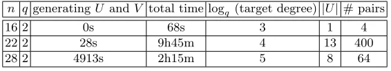
Practical Results. We have implemented Algorithm 2 inside the MAGMA computer algebra sys-tem[13], running on one core of a 2.8 Ghz Xeon machine. As shown in Table 1, we found out that in practice it is difficult to balance the cost of building U and V on the one hand, and going through the candidate pair on the other hand, because the target degree can only take √n integer values. We could nevertheless verify in practice that the complexity of building the lists and the expected number of right pairs in them is consistent with our expectations. The source code is in the public domain, and is available on the webpage of the first author. It uses an unpublished algorithm to solve the inhomogeneous instances.
n q generatingU andV total time logq (target degree)|U|# pairs
16 2 0s 68s 3 1 4
22 2 28s 9h45m 4 13 400
28 2 4913s 2h15m 5 8 64
Table 1.Experimental results on Algorithm 2.
5 Map Your Neighborhood: A Faster Graph-And-Birthday Algorithm
We have seen in section 3 that the linearity graphs, once deprived from the “zero” vertex, contain many small connected components. Of course, if y =Sx, then the connected component ofx is isomorphic to the connected component of y. In this section, we describe an algorithm that builds upon this idea—instead of just looking at immediate neighbors, as we did in algorithm 2, we now try to look at the whole connected component, in order to distinguish between vertices of the same degree.
Canonical Graph Labeling. Given a graph G, a Canonical Labeling algorithm relabels the ver-tices of G, thus producing a graph Canon(G), which is by definition isomorphic to G. The result is canonical in the sense that if G and H are isomorphic graphs, then Canon(G) = Canon(H). The canonical labels are therefore complete invariants of the isomorphism class, and as such, computing a canonical labeling is necessarily harder than checking if two graphs are isomorphic. However, com-puting a canonical labeling can be done in average linear time [6], because except for an exponentially small fraction of all graphs, it can be done with a very simple linear algorithm. Deterministic algo-rithms that always succeed are subexponential, with complexity O exp √nlogn [5]. The perhaps most well-known, and most practical algorithm dates back to 1978, and is implemented in the nauty
open-source package [38]. It is known to be exponential on some specific counter-examples [39], but otherwise performs exceptionally well. There are also many relevant classes of graphs where canon-ical labeling is polynomial [26]: graphs of bounded degree, planar graphs, chordal graphs, graphs of bounded treewidth, etc.
“hash function”. In fact, in algorithm 2, we used the degree as such a “hash function”, but it was not very discriminating, because the degree does not contain enough entropy. We hope that H behaves as a good hash function, and that false positives,i.e., pairs (x, y) such that H(x) =H(y) but y 6=Sx, should be very rare.
One problem is thatH does not distinguish between vertices of the same connected component. To improve it, we would need a way to single out a specific vertex in the connected component. Fortunately, most canonical labeling algorithm return the isomorphism (sayρ) between their argument G andCanon(G). To single a vertexx out inG, it is sufficient to sendρ(x) along with the canonical labeling of G.
A Canonical-Labeling-Based Algorithm As discussed in section 3,G∗f contains many small con-nected components that are all isomorphic to each others, since they are all cliques of size q−1. Therefore, if we want our “hash function” to be discriminating, we must avoid small connected com-ponents. Our “hash function” will thus reject the vector x if there is no simple path starting from x and of length at least r. In the other direction, we cannot exclude the existence of a giant connected component of exponential size. Therefore, we only consider the radius-r neighborhood of the vertexx we are interested in,i.e., the set of all vertices that can be reached fromxby crossing at mostr edges. This is the basis of algorithm 3.
Algorithm 3 Canonical Labeling/Birthday Based Algorithm 1: functionHashable[r](G, x)
2: Perform a Breadth-First Search inGstarting fromx
3: returnTrueif the BFS hits a vertexredges away fromx
4: functionH[r](G, x)
5: Cx←subgraph ofGformed by all vertices at mostredges away fromx. 6: ρ,G ←CanonicalLabeling(Cx)
7: return G, ρ(x)
8: functionSampleHashTable(h) 9: L← ∅
10: repeat
11: repeat
12: x←random vertex ofG∗h
13: untilHashable[r](G∗h, x)
14: LhH[r](G∗h, x))
i ←x
15: until |L|=√2qn/2
16: returnL
17: functionCanonical-Labeling-QMLE(f, g) 18: U ←SampleHashTable(f)
19: V ←SampleHashTable(g)
20: for all(h17→x)∈U,(h27→y)∈V such thath1=h2 do 21: f0(z)←f(z+y)
22: g0(z)←g(z+x)
Remarks on Algorithm 3. Establishing the complexity and success probability of algorithm 3 is surprisingly difficult, probably because is relies on topological properties of G∗f, which is a somewhat random but very structured graph.
Algorithm 3 has been written in a generic way, independently of the actual value ofq. However, we have only been able to discuss its properties when q = 2. We have verified that the algorithm works as we expected in this case, but the situation whenq 6= 2 is not so clear. We tend to believe that the complexity and/or success probability degrade exponentially fast when q grows, but we fall short of definitive conclusion.
When q = 2, the structure of G∗f seems to be richer. For instance, we already alluded to the fact that the fraction of nodes whose connected component is of size only q−1, grows like 1−1/q2. In addition, as we will see in the next section, setting q = 2 allows us to turn most more-or-less-random graphs into trees, which are much easier to deal with.
Preliminary Analysis of Algorithm 3. When q = 2, the correctness of the algorithm is implied by the following three heuristic statements.
Claim. i) Hashable[r] G∗f, x
is true with probability≈1/rover the random choice off (assuming x6= 0).
ii) BothHashable[r]and H[r] can be evaluated in expected time O rn3.
iii) When restricted to elements that are Hashable[r], then H[r]
G∗f,· is an εr-almost universal hash function family (indexed by f) for some ε <1.
The notion of almost universal hash function is usually useful when the hash function is “less injective” than a random function. In this paper though, H[r] can become more injective than a
random function, as soon as r becomes sufficiently large.
It follows from claimithat the expected number of iterations of the loop of lines 11–13 isO(r), and it follows from claim ii that finding one admissible vectorx requires O r2n3 operations on average. Claim iii then guarantees that if we choose r to be a bit larger than n, then the probability to find hash collisions can be made smaller than 2−n, and standard birthday-type results guarantee that the number of expected hash collisions in the execution of SampleHashTableis constant. From this, we
conclude that SampleHashTableruns in expected time O r2n3qn/2.
It follows from the birthday paradox [53] that there is a “right pair” in U ×V, i.e., a pair (x, y) withy=Sx, with probability greater than 1−1/e. This is because (Fq)nhasqn elements and that the sizes of both U and V are essentiallyqn/2. This guarantees the success probability of the algorithm.
Let us denote byN the number of bogus inhomogeneous queries,i.e., the number of pairsx6=y∈ U×V with the same hash. It follows from Markov’s inequality and claimiiithatP[N ≥1]≤2qn·εr. Thus, as soon as r is asymptotically larger than n, e.g. r = nlog logn, then the probability that N ≥ 1 gets exponentially small. This concludes our preliminary analysis: algorithm 3 runs in time O n5qn/2, and sends a constant number of inhomogeneous queries. It now remains to show that our claims are valid, but we first find it reassuring to show that the practical behavior of the algorithm is very consistent with our expectations.
n qgeneratingU andV finding collisions |U| N
16 2 3.6 s 1s 64 6
24 2 123 s 13s 836 5
32 2 61 min 200s 11585 2
40 2 31 h 2h 165794 7
Table 2.Experimental results on Algorithm 3
6 Discussion of the Claims
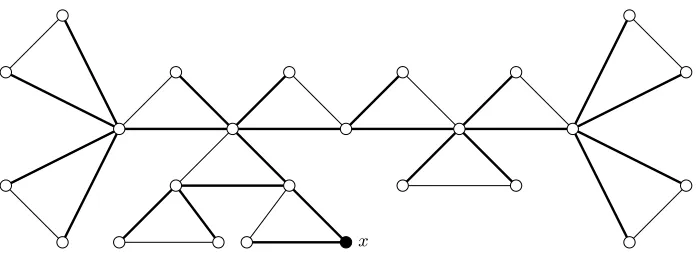
Special Structure in Linearity Graphs. Any analysis of algorithm 3 will have to rely on the properties of linearity graphs. As argued above, the situation when q = 2 is somewhat different than that obtained with larger values of q. When q = 2, the connected components of G∗f seem to enjoy a very nice structure, as illustrated by figure 1. The origin of the triangles is that any non-isolated vertexxbelong to the (q2−1)-clique formed byx,yandx+y(0 has been removed). If it were not for these triangles, the connected components ofG∗f would be trees. While this structure is clearly visible on all the examples we could forge, we fall short of any rigorous explanation.
x
Fig. 1.A typical moderate-size connected component ofG∗f whenq= 2. Self-edges are not shown. The thick edges show
a spanning tree obtained by performing a Breadth-First Search starting fromx.
Conjecture 1. When r is polynomial in n, then with high probability the radius-r neighborhood of any vertex in G∗f does not contain cliques of size strictly greater than q2−1. In addition, every edge
belongs to at most one maximal clique with high probability.
Back to the Trees. Fig. 1 illustrates that the connected components are close to trees, and this analogy can easily be made rigorous when q= 2. To a vertex x in a linearity graph G∗f, we associate the unordered, unlabeled treeT[r](G∗f, x) by performing a Breadth-First Search inG∗f starting fromx, and stopping r edges away from x. It is well-known that any graph traversal induces a spanning tree of the graph. The treeT[r](G∗f, x) is simply the spanning tree induced by the BFS (cf. fig. 1).
Lemma 3. If G1, G2 satisfy the properties of Conjecture 1, then:
(G1, x) isomorphic to(G2, y) ⇐⇒ ∀r. T[r](G∗1, x) isomorphic toT[r](G
∗
2, y)
algorithm 3. Indeed,Hashable[r](G, x) can be evaluated by checking ifT[r](G, x) has depthr. Lastly,
it is well-known that unordered, unlabeled trees can be canonically labeled in linear time thanks to a venerable algorithm of Aho, Hopcroft and Ullman [2]. .
Random Trees From Random Linearity Graphs. Whenf is randomly chosen, then T[r](G∗f, x) can also be seen as a random variable. Because each vertex ofG∗f haskneighbors with some probability, then each node of T[r](G∗f, x) also has a given number of children (sometimes called “offspring” in the context of branching processes) with some probability. Everything looks as ifT[r](G∗f, x) were a random tree where the number of descendant of each node was chosen at random according to a given offspring distribution. The offspring distribution of xinT[r](G∗f, x) (i.e., the root of the tree) is almost exactly the degree distribution ofG∗f, which is known by lemma 2 (with the caveat that self-loops are removed). However, the offspring distribution of non-root nodes is a bit different:
`n(i) =P[a non-root node produces ioffspring] =
(
pn,k when i=qk−q2
0 otherwise
where
pn,k =Pdim kerDxf =k
y∈kerDxf
= λ(n)λ(n−2) λ(k)λ(k−2)λ(n−k) ·q
−k(k−2)
The expression of pn,k can be derived from a reasoning similar to that of the proof of lemma 2, which can also be found in [21]. It is also possible to compute theexpected progeny µof each non-root node, and the varianceσ2 of the offspring distribution :
µ= 1− 1
qn−2 σ
2 =q2(q−1)
1−q
2+ 1
qn + q2 q2n
These two expressions can be derived from the expectation and the variance of the degree in Gf without too much effort.
When a random tree is sampled by choosing independently the number of children of each node according to a fixed law, the resulting object is called a random Galton-Watson tree. These random trees are well-studied [4], and this wealth of results would be extremely useful to our own purposes. Unfortunately, inT[r](G∗f, x), the number of descendant of each node is not even pairwise-independent. We nevertheless denote byPn the law of Galton-Watson trees with offspring distribution `n, and by P[nr] the law of such trees conditioned to be of height at least r. We verified in practice that the following assumption holds very well.
Heuristic Assumption: Over the random choice off,T[r](G∗f, x) has the same properties as Galton-Watson trees sampled according to P[nr] and truncated at depthr.
Becauseµ≤1, trees sampled according to Pn are finite with probability one [4]. In addition, the probability that a tree sampled according to Pn has height greater than r is equivalent to 2/(rσ2)≈ 2/(r·q3) [4]. This justifies claimi.
However, it follows from this result that the expected height of trees sampled according to Pn is not finite; this justifies why we stop the BFS after a (finite) depth. It is also known that in trees sampled according toPn, the expected total number of nodes afterhgeneration ish+ 1 [42]. It follows that actually performing the BFS requires on averageO(r) matrix operations. This justifies claimii.
False Positive Rate. It remains to justify claim iii, the trickiest one. Under the heuristic assump-tion that T[r](G∗
probability that two random trees sampled according toP[nr] are isomorphic decreases exponentially fast with r.
In other word, we must determine the probability that two random trees are isomorphic. While this appears to be a natural question, it has (to the best of our knowledge) not been treated in the literature. We could not establish the required exponential upper-bound in general, however we proved a strong enough bound that holds if we are allowed to reject a negligible amount of trees (i.e., shrinking a bit theHashable[r] domain).
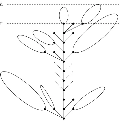
We say that a tree has aunique spine decomposition if there is a unique path starting from the root and reaching a leaf of maximal depth. We also say that a tree has a unique spine decompositionup to height k if there is a unique path starting from the root and reaching depth kthat extends to a path reaching nodes of maximal depth. Fig 2 shows a tree with a spine decomposition up to a certain level. Note that it is easy (and efficient) to check whether a given tree has this property. We now redefine the hashable domain by saying thatx∈GisHashable[h,r]if and only ifT[h](G, x) has depth at least
h, and admits a unique spine decomposition up to heightr.
h
r
Fig. 2.A Tree of heighthwith a spine decomposition up heightr.
Theorem 2. There exists constantsc, dsuch that the probability that a random tree sampled according to P[nh] has a spine decomposition up to height r is greater than 1−c·(r/h)−c/r.
Informally speaking, this theorem means than enforcing the existence of a unique spine decom-position up to some height does not really shrink the hashable domain. For instance, one may pick h=nlognand r=nlog logn. With these values, trees of height hhave a unique spine decomposition up to heightr asymptotically almost surely.
Theorem 3. There is a constant ε ∈]0; 1[ such that if two trees sampled according to P[nh] have a unique spine decomposition up to height r, then the probability that they are isomorphic is upper-bounded by εr.
unique spine decomposition under height r, with h = nlogn and r = nlog logn is enough to make algorithm 3 work as advertised.
References
1. Agrawal, M., Saxena, N.: Equivalence of f-algebras and cubic forms. In Durand, B., Thomas, W., eds.: STACS. Volume 3884 of Lecture Notes in Computer Science., Springer (2006) 115–126
2. Aho, A.V., Hopcroft, J.E., Ullman, J.D.: The Design and Analysis of Computer Algorithms. Addison-Wesley Publishing Company (1974)
3. Alon, N., Blais, E.: Testing boolean function isomorphism. In Serna, M.J., Shaltiel, R., Jansen, K., Rolim, J.D.P., eds.: APPROX-RANDOM. Volume 6302 of Lecture Notes in Computer Science., Springer (2010) 394–405
4. Athreya, K.B., Ney, P.: Branching processes. Springer-Verlag, Berlin, New York, (1972)
5. Babai, L., Kantor, W.M., Luks, E.M.: Computational complexity and the classification of finite simple groups. In: FOCS, IEEE Computer Society (1983) 162–171
6. Babai, L., Kucera, L.: Canonical labelling of graphs in linear average time. In: FOCS, IEEE Computer Society (1979) 39–46
7. Baena, J., Clough, C., Ding, J.: Square-vinegar signature scheme. In: PQCrypto ’08: Proceedings of the 2nd International Workshop on Post-Quantum Cryptography, Berlin, Heidelberg, Springer-Verlag (2008) 17–30
8. Bardet, M., Faug`ere, J.C., Salvy, B.: On the complexity of Gr¨obner basis computation of semi-regular overdetermined algebraic equations. In: Proc. International Conference on Polynomial System Solving (ICPSS). (2004) 71–75 9. Bettale, L., Faug`ere, J.C., Perret, L.: Cryptanalysis of the trms signature scheme of pkc’05. In Vaudenay, S., ed.:
AFRICACRYPT. Volume 5023 of Lecture Notes in Computer Science., Springer (2008) 143–155
10. Billet, O., Gilbert, H.: A traceable block cipher. In Laih, C.S., ed.: ASIACRYPT. Volume 2894 of Lecture Notes in Computer Science., Springer (2003) 331–346
11. Billet, O., Macario-Rat, G.: Cryptanalysis of the square cryptosystems. In Matsui, M., ed.: ASIACRYPT. Volume 5912 of Lecture Notes in Computer Science., Springer (2009) 451–468
12. Biryukov, A., Canni`ere, C.D., Braeken, A., Preneel, B.: A toolbox for cryptanalysis: Linear and affine equivalence algorithms. In: EUROCRYPT. (2003) 33–50
13. Bosma, W., Cannon, J.J., Playoust, C.: The Magma Algebra System I: The User Language. J. Symb. Comput. 24(3/4) (1997) 235–265
14. Bouillaguet, C., Faug`ere, J.C., Fouque, P.A., Perret, L.: Practical cryptanalysis of the identification scheme based on the isomorphism of polynomial with one secret problem. In Catalano, D., Fazio, N., Gennaro, R., Nicolosi, A., eds.: Public Key Cryptography. Volume 6571 of Lecture Notes in Computer Science., Springer (2011) 473–493 15. Clough, C., Baena, J., Ding, J., Yang, B.Y., Chen, M.S.: Square, a new multivariate encryption scheme. In Fischlin,
M., ed.: CT-RSA. Volume 5473 of Lecture Notes in Computer Science., Springer (2009) 252–264
16. Cramer, R., ed.: Advances in Cryptology - EUROCRYPT 2005, 24th Annual International Conference on the Theory and Applications of Cryptographic Techniques, Aarhus, Denmark, May 22-26, 2005, Proceedings. In Cramer, R., ed.: EUROCRYPT’05. Volume 3494 of Lecture Notes in Computer Science., Springer (2005)
17. Daemen, J.: Limitations of the even-mansour construction. [34] 495–498
18. Ding, J., Wolf, C., Yang, B.Y.: -invertible cycles for multivariate quadratic public key cryptography`. In Okamoto, T., Wang, X., eds.: Public Key Cryptography. Volume 4450 of Lecture Notes in Computer Science., Springer (2007) 266–281
19. Dubois, V., Fouque, P.A., Shamir, A., Stern, J.: Practical Cryptanalysis of SFLASH. In: CRYPTO. Volume 4622., Springer (2007) 1–12
20. Dubois, V., Fouque, P.A., Stern, J.: Cryptanalysis of SFLASH with Slightly Modified Parameters. In: EUROCRYPT. Volume 4515., Springer (2007) 264–275
21. Dubois, V., Granboulan, L., Stern, J.: An efficient provable distinguisher for hfe. In Bugliesi, M., Preneel, B., Sassone, V., Wegener, I., eds.: ICALP (2). Volume 4052 of Lecture Notes in Computer Science., Springer (2006) 156–167 22. Dunkelman, O., Keller, N., Shamir, A.: Minimalism in cryptography: The even-mansour scheme revisited. In
Pointcheval, D., Johansson, T., eds.: EUROCRYPT. Volume 7237 of Lecture Notes in Computer Science., Springer (2012) 336–354
23. Even, S., Mansour, Y.: A construction of a cioher from a single pseudorandom permutation. [34] 210–224
24. Faug`ere, J.C., Joux, A., Perret, L., Treger, J.: Cryptanalysis of the hidden matrix cryptosystem. In Abdalla, M., Barreto, P.S.L.M., eds.: LATINCRYPT. Volume 6212 of Lecture Notes in Computer Science., Springer (2010) 241–254
25. Faug`ere, J.C., Perret, L.: Polynomial Equivalence Problems: Algorithmic and Theoretical Aspects. In Vaudenay, S., ed.: EUROCRYPT. Volume 4004 of Lecture Notes in Computer Science., Springer (2006) 30–47
26. Fortin, S.: The graph isomorphism problem. Technical report, University of Alberta (1996)
28. Fouque, P.A., Macario-Rat, G., Perret, L., Stern, J.: Total break of the`-ic signature scheme. In Cramer, R., ed.: Public Key Cryptography. Volume 4939 of Lecture Notes in Computer Science., Springer (2008) 1–17
29. Fouque, P.A., Macario-Rat, G., Stern, J.: Key Recovery on Hidden Monomial Multivariate Schemes. In Smart, N.P., ed.: EUROCRYPT. Volume 4965 of Lecture Notes in Computer Science., Springer (2008) 19–30
30. Geiger, J.: Elementary new proofs of classical limit theorems for Galton-Watson processes. J. Appl. Probab.36(2) (1999) 301–309
31. Geiselmann, W., Meier, W., Steinwandt, R.: An Attack on the Isomorphisms of Polynomials Problem with One Secret. Int. J. Inf. Sec.2(1) (2003) 59–64
32. Gligoroski, D., Markovski, S., Knapskog, S.J.: Multivariate quadratic trapdoor functions based on multivariate quadratic quasigroups. In: Proceedings of the American Conference on Applied Mathematics, Stevens Point, Wis-consin, USA, World Scientific and Engineering Academy and Society (WSEAS) (2008) 44–49
33. Goldreich, O., Micali, S., Wigderson, A.: Proofs that yield nothing but their validity and a methodology of crypto-graphic protocol design (extended abstract). In: FOCS, IEEE (1986) 174–187
34. Imai, H., Rivest, R.L., Matsumoto, T., eds.: Advances in Cryptology - ASIACRYPT ’91, International Conference on the Theory and Applications of Cryptology, Fujiyoshida, Japan, November 11-14, 1991, Proceedings. In Imai, H., Rivest, R.L., Matsumoto, T., eds.: ASIACRYPT. Volume 739 of Lecture Notes in Computer Science., Springer (1993)
35. Joux, A., Kunz-Jacques, S., Muller, F., Ricordel, P.M.: Cryptanalysis of the tractable rational map cryptosystem. [54] 258–274
36. Kayal, N.: Efficient algorithms for some special cases of the polynomial equivalence problem. In Randall, D., ed.: SODA, SIAM (2011) 1409–1421
37. Macario-Rat, G.: Cryptanalyse de sch´emas multivari´es et r´esolution du probl`eme Isomorphisme de Polynˆomes. PhD thesis, Universit´e Paris Diderot — Paris 7 (June 2010)
38. McKay, B.: Computing automorphisms and canonical labelling of graphs. In: Lecture Notes in Mathematics. (1978) 223–232
39. Miyazaki, T.: The complexity of mckay’s canonical labelling algorithm. In Finkelstein, L., Kantor, W.M., eds.: Groups and computation, II. Volume 28 of DIMACS: Series in Discrete Mathematics and Theoretical Computer Science., AMS and DIMACS (1997) 239–256
40. Mohamed, M., Ding, J., Buchmann, J., Werner, F.: Algebraic attack on the mqq public key cryptosystem. In Garay, J., Miyaji, A., Otsuka, A., eds.: Cryptology and Network Security. Volume 5888 of Lecture Notes in Computer Science. Springer Berlin / Heidelberg (2009) 392–401
41. Monagan, M.B., Geddes, K.O., Heal, K.M., Labahn, G., Vorkoetter, S.M., McCarron, J., DeMarco, P.: Maple 10 Programming Guide. Maplesoft, Waterloo ON, Canada (2005)
42. Pakes, A.G.: Some limit theorems for the total progeny of a branching process. Advances in Applied Probability 3(1) (1971) 176–192
43. Patarin, J.: Hidden fields equations (hfe) and isomorphisms of polynomials (ip): Two new families of asymmetric algorithms. In: EUROCRYPT. (1996) 33–48
44. Patarin, J., Goubin, L., Courtois, N.: Improved Algorithms for Isomorphisms of Polynomials. In: EUROCRYPT. (1998) 184–200
45. Patarin, J., Goubin, L., Courtois, N.: Improved Algorithms for Isomorphisms of Polynomials – Extended Version. available athttp://minrank.org/ip6long.pdf(1998)
46. Perret, L.: A Fast Cryptanalysis of the Isomorphism of Polynomials with One Secret Problem. [16] 354–370 47. Pointcheval, D.: A new identification scheme based on the perceptrons problem. In: EUROCRYPT. (1995) 319–328 48. Sakumoto, K.: Public-key identification schemes based on multivariate cubic polynomials. In Fischlin, M., Buchmann, J., Manulis, M., eds.: Public Key Cryptography. Volume 7293 of Lecture Notes in Computer Science., Springer (2012) 172–189
49. Sakumoto, K., Shirai, T., Hiwatari, H.: Public-key identification schemes based on multivariate quadratic polynomi-als. In Rogaway, P., ed.: CRYPTO. Volume 6841 of Lecture Notes in Computer Science., Springer (2011) 706–723 50. Shamir, A.: An efficient identification scheme based on permuted kernels (extended abstract). In Brassard, G., ed.:
CRYPTO. Volume 435 of Lecture Notes in Computer Science., Springer (1989) 606–609
51. Stern, J.: A new identification scheme based on syndrome decoding. In Stinson, D.R., ed.: CRYPTO. Volume 773 of Lecture Notes in Computer Science., Springer (1993) 13–21
52. Stern, J.: Designing identification schemes with keys of short size. In Desmedt, Y., ed.: CRYPTO. Volume 839 of Lecture Notes in Computer Science., Springer (1994) 164–173
53. Vaudenay, S.: A Classical Introduction to Cryptography: Applications for Communications Security. Springer-Verlag New York, Inc., Secaucus, NJ, USA (2005)
54. Vaudenay, S., ed.: Public Key Cryptography - PKC 2005, 8th International Workshop on Theory and Practice in Public Key Cryptography, Les Diablerets, Switzerland, January 23-26, 2005, Proceedings. In Vaudenay, S., ed.: Public Key Cryptography. Volume 3386 of Lecture Notes in Computer Science., Springer (2005)
55. Wang, L.C., Hu, Y.H., Lai, F., yen Chou, C., Yang, B.Y.: Tractable rational map signature. [54] 244–257
A Expected Progeny and Variance
By definition the expected progeny is:
µ= n X k=2 pn,k
qk−q2
Via an analog of lemma 2, this can be rephrased in terms of the properties of a random linear map h. Indeed, it is shown in [21] that:
pn,k =Pdim kerDxf =ky∈kerDxf
=Pdim kerh=kx, y∈kerh And therefore: µ= n X k=2
Pdim kerh=kx, y∈kerh
qk
!
−q2
The sum is in fact the expected cardinality of the kernel of a random linear map known to vanish on a fixed 2-dimensional subspace:
µ=Ecard kerhx, y∈kerf
−q2
Thus, to establish the expression ofµ, we determine the expected cardinality of the kernel of a random linear maph known to vanish on a fixed subspaceF of dimension s. Even though this seems to be an elementary question, we could not find the result in the existing literature.
Lemma 4. Leth be a uniformly random endomorphism of(Fq)n, vanishing on a subspaceF of (Fq)n, with dimF =s. Then:
Ecard kerhF ⊆kerf
=qs+ 1− 1 qn−s
This lemma establishes the expression of µ (and we postpone its proof a little bit). Let us now turn our attention to the varianceσ2:
σ2 =
" n X
k=2
pn,k
qk−q22
#
−µ2
= n
X
k=2
pn,k·q2k
!
−2q2 n
X
k=2
pn,k·qk
!
+q4−µ2
= n
X
k=2
pn,k·q2k
!
− n
X
k=2
pn,k·qk
!2
Thanks to the relation betweenpn,k and random linear maps outlined above, we see that σ2 is in fact exactly the variance of the cardinality of the kernel of a random linear map known to vanish on two fixed vectors.
Lemma 5. Leth be a uniformly random endomorphism of(Fq)n, vanishing on a subspaceF of (Fq)n, with dimF =s. Then the variance of the cardinality of its kernel is:
qs(q−1)
1− q s+ 1
qn + qs q2n
Proof (of lemma 4).
En=Ecard kerfF ⊆kerf
= n
X
k=s
Pdim kerf =kF ⊆kerf
qk
= n
X
k=s
λ(n)λ(n−s) λ(k)λ(k−s)λ(n−k)q
−k(k−s)qk
A combinatorial and/or elementary argument completely eluded us. We therefore use the method of “creative telescoping” to establish the result by induction onn. First, we notice that the announced results holds whenn=s. Let us therefore assumen > s. We denote byT(n, k, s) the hairy term under the sum. It is a q-hypergeometric term because if we set X = qn and Y = qk, we see that the two following ratios are rational functions of X and Y:
T(n+ 1, k, s) T(n, k, s) =
q2X2−(q+qs+1)X+qs q2X2−qXY
T(n, k+ 1, s) T(n, k, s) =q
s+2 X+Y
X(qY −qs) (qY −1)
We thus used the q-analog of Zeilberger’s algorithm [56] (as implemented in Maple [41]), and it found the nice recurrence relation:
a·T(n+ 1, k, s)−b·T(n, k, s) =g(n, k+ 1, s)−g(n, k, s) (?)
where:
a=qn+1+qn+s+1−qs+1
b=qn+1+qn+1+s−qs
g(n, k, s) = q k−qs
qk−1 qn+s+1−qn+s+2−qk+s+qn+k+1+qn+k+s+1
q2k(qn+1−qk) T(n, k, s)
The point is that summing (?) over k=s, . . . , n−1 yields:
a(En+1−T(n+ 1, n+ 1, s)−T(n+ 1, n, s))−b(En−T(n, n, s)) =g(n, n, s)−g(n, s, s)
At this point, it is easy to find that g(n, s, s) = 0, and we check (using a computer algebra system!) that:
g(n, n, s) +a·(T(n+ 1, n+ 1, s) +T(n+ 1, n, s)) +b·T(n, n, s) = 0
Thus, we have established that:
1 +qs− 1 qn−s
En+1 =
1 +qs− 1 qn+1−s
En
Thus, if the result holds at rankn, then it also holds at rank n+ 1. ut
Proof (of lemma 5). The variance is:
Vn= n
X
k=s
λ(n)λ(n−s) λ(k)λ(k−s)λ(n−k)q
−k(k−s)
q2k
| {z }
Un
−
qs+ 1− 1 qn−s
We will first demonstrate by induction on n≥sthat:
Un=q2s+ 1 + (1 +q)
qs− 1 qn−s −
1 qn−2s
+ 1
q2n−1−2s (♣)
When n=s, we should haveUn=q2n, and looking at (♣) carefully reveals that our expression ofUn simplifies to this value. Let us therefore assumen > s, and let us again denote byT(n, k, s) the hairy term under the sum. It is again a q-hypergeometric term, and running the q-analog of Zeilberger’s algorithm yields:
a·T(n+ 1, k, s)−b·T(n, k, s) =g(n, k, s)−g(n, k+ 1, s) (?)
where:
a=−qn+s+2+qs+1+2n+q1+2n+q2s+2−q2s+n+1−qs+1+n−q2s+2+n+q2s+2n+1+qs+2+2n
b=−q1+2n+qn+s−qs+1+2n+qs+1+n−q2s+q2s+n+1+q2s+n−q2s+2n+1−qs+2+2n
g is a complicated term with a singularity when n+ 1 =k. We again notice that g(n, s, s) = 0 and that:
a·T(n+ 1, n+ 1, s) +a·T(n+ 1, n, s)−b·T(n, n, s) =g(n, n, s)
So that summing (?) over k=s, . . . , n−1 and exploiting the previous equation yields:
a·Un+1 =b·Un
By induction hypothesis, (♣) holds at rank n. Plugging the expression of Un into this recurrence relation and simplifying shows that (♣) holds at rank n+ 1 — please use a computer algebra system if you really want to verify this. Moving back to the expression ofVn, it is not difficult to verify that
the result of the lemma holds. ut
B Isomorphism of Random Trees
For anyn≥3, letTbe a tree sampled according toP(i.e., with offspring distribution`), and letP[h] be the law of Tconditioned to have height at least h.
In this section, all quantities depend onn(the random treeT, the lawP[h], the offspring distribution `, the heighth, etc.), but we do not always make this dependency explicitly visible by writing subscripts or superscripts, in order to make notations less cumbersome. In addition, we also write P[h][·] instead of P·Height(T)≥h
.
We need a criterion to decide whether two conditioned trees are isomorphic or not, and we need it to be simple enough so that we may evaluate the probability that it holds. The criterion we will use is the following: two isomorphic trees with a unique spine decomposition must have empty subtrees emanating from the backbone at the exact same heights. Of course, if the spine decomposition is unique up to heightr, then this holds only up to heightr. This will intuitively show that two random trees with a unique spine decomposition up to height r are isomorphic with a probability that gets exponentially small in r. We will make this intuition formal later, but we must first introduce some properties of the spine decomposition.
Fig. 3.Illustration of the spine decomposition (this is Figure 1 from [30]). This shows the Galton-Watson tree conditionned on non-extinction at generationnandn+ 1 respectively.GW(k) denotes a Galton-Watson tree conditioned to be extinct at generation k. The subtrees to the right of the line of descent of the left-most particle are ordinary Galton-Watson trees.
Let us work for a moment with ordered Galton-Watson trees. That is, we also record who is the descendant of each parent and offspring are ordered (so that we can talk about brothers to the left or to the right of an individual). In [30], Geiger shows that if we define the sequence of independent random variables (Vm, Ym), m∈N by
P[Vm =j, Ym =k] = P[Height(T)
≥m−1]
P[Height(T)≥m] ·P[Height(T)< m−1]
j−1·
`(k),
for 1 ≤ j ≤ k <∞, then Tn conditioned to have height at least h has the same law as the random tree constructed inductively as follows:
– The root (i.e., the first node of the spine) hasYh offspring.
– To each of theVh−1 first offspring node we graft a Galton-Watson tree with offspring distribution `and conditioned to have height (strictly) less than h−1. These Vh−1 trees are independent of each other (and of the rest of the construction). These subtrees are on the left of the backbone on fig. 3.
– To each of theYh−Vh last offspring, we graft an unconditioned Galton-Watson tree with offspring distribution`(again, these trees are independent of each other and of the rest of the construction). These subtrees are on the right of the backbone on fig. 3.
– The Vh-th offspring node continues the spine. It has Yh−1 offspring, the first Vh−1 ones are the
roots of i.i.d. Galton-Watson trees conditioned to have height less thanh−2, the lastYh−1−Vh−1
are the roots of i.i.d. unconditioned Galton-Watson trees and the spine carries on with theVh−1-th
offspring, which hasYh−2 offspring nodes, and so on.
Observe that the marginal distribution ofYm is given by
P[Ym =y] =
1−P[Height(T)< m−1]y
P[Height(T)≥m]
The spine can be seen as a “prolific” line of descent that survives up to generationhby producing a bi-ased number of offspring, while the other individuals of the population reproduce essentially according to the initial offspring distribution (we refer to [30] for an explanation of the fact that trees emanating from brothers to the left of the spine are conditioned not to have descendants at generationh).
Proof (proof of theorem 2). We show that in a tree sampled according to P[h], with high probability only one path from the root to height r extends to a path reaching heighth. Call this eventA. Since this property is purely topological, then it does not matter whether the tree is ordered or not. We obtain the desired result by bounding from below the probability ofAby the probability that all trees emanating from the spine under heightr are of height less thanh−r. The independence of this family of trees, together with the fact (easy to check) that for every integer iin the interval{1, . . . , r−1}
PHeight(T)< h−rHeight(T)< h−i
≥P[Height(T)< h−r],
enables us to write
P[A]≥ r−1 Y
i=0
E
h
P[Height(T)< h−r]Yh−i−1
i
≥E
h
P[Height(T)< h−r]
Pr−1
i=0Yh−ii. (2)
Now, asn→+∞, all thepn,k(fork∈ {3, . . . , n}) converge to a finite limitp∞,k , the expected progeny µconverges to 1 (recall thatµ <1 for every n), and finally the variance σn2 converges toq3−q2. The last two convergences happen exponentially fast inn, therefore the same proof as that of Theorem 3.1 in [30] (in whichµ= 1 for alln) shows that whenever (mn)n≥1 tends to infinity at most polynomially,
we have
lim
n→∞mn·P[Height(T)≥mn] =
2
σ2. (3)
Furthermore, we have the following lemma.
Lemma 6. There exist constants C3, C4 >0 such that for every n≥3,
P
"r−1 X
i=0
Yh−i> rC3 #
≤ C4 r .
We postpone the proof of Lemma 6 until the end of the proof of Theorem 2. Armed with (3) and Lemma 6, we can come back to (2) and write for every n
P[A]≥E
h
P[Height(T)< h−r]rC3·1{Pr−1
i=0Yh−i≤C3r} i
≥
1− C4 σ2h
rC3
×P
"r−1 X
i=0
Yh−i≤rC3 #
≥e−hrC6
1−C4 r
≥1− r
hC7. (4)
Proof (of lemma 6). We use Markov’s inequality (in a Chebychev-like fashion) as follows: ifC3 >0,
we have for each n≥3
P
"r−1 X
i=0
Yh−i > rC3 #
=P
"r−1 X
i=0
(Yh−i−E[Yh−i])> C3·r−
r−1 X
i=0
E[Yh−i]
#
≤ E
r−1 X
i=0
(Yh−i−E[Yh−i])
!2
C3·r−
r−1 X
i=0
E[Yh−i]
!2 . (5)
Let us show that the numerator in the right-hand side of (5) is of order r, while the denominator is of order r2 whenever C
3 > 0 is large enough. These two points rely on appropriate bounds on the
first two moments of all Yh−i’s (observe that the numerator is in fact the sum of the variances of the Yh−i’s). Indeed, recall from (1) that for everyk∈ {3, . . . , n},
P
h
Yh−i=qk−q2
i
= 1−P[Height(T)< h−i−1] qk−q2
P[Height(T)≥h−i] ·pn,k
and these are the only possible values for Yh−i. Because 1−e−x ≤ x for all x ≥ 0, we can write for everyi≤r−1 :
1−P[Height(T)< h−i−1]qk−q2 ≤ −qk−q2
logP[Height(T)< h−i−1]
≤ −qk−q2logP[Height(T)< h−r−2].
We thus have for every such integeri
1−P[Height(T)< h−i−1]q
k−q2
(qk−q2)·
P[Height(T)≥h−i] ≤ −
logP[Height(T)< h−r−2]
P[Height(T)≥h] .
Moreover, because λ(·) is decreasing,
λ(n)λ(n−2)
λ(k)λ(k−2)λ(n−k) ≤nlim→∞
1
λ(n) =:Cq.
Combining the above, we arrive at
P
h
Yh−i =qk−q2
i
≤ −logP[Height(T)< h−r−2] P[Height(T)≥h]
·Cq·
qk−q2q−k(k−2)
for everyn≥3 andk∈ {2, . . . , n}. This yields
E[Yh−i]≤ −
logP[Height(T)< h−r−2]
P[Height(T)≥h] ·Cq·
n
X
k=3
qk−q22q−k(k−2)
E
h
(Yh−i)2
i
≤ −logP[Height(T)< h−r−2]
P[Height(T)≥h] ·Cq·
n
X
k=2
qk−q23q−k(k−2)
Now, by (3) we have
lim n→∞−
logP[Height(T)< h−r−2]
and furthermore,
∞
X
k=3
qk−q22q−k(k−2) =:m1 <∞ and
∞
X
k=3
qk−q23q−k(k−2)=:m2<∞.
As a consequence, there exists C >0 such that for every n≥3, we have
r−1 X
i=0
E[Yh−i]≤Cm1r,
and (using the independence of all Ym’s)
E
r−1 X
i=0
Yh−i−E[Yh−i]
!2
=
r−1 X
i=0
Var (Yh−i)≤rC0,
for a constant C0 > 0 depending on m1 and m2. Choosing C3 > Cm1 and coming back to (5), we
obtain the existence ofC4 >0 such that for everyn≥3,
P
"r−1 X
i=0
Yh−i≥rC3 #
≤ C4 r .
This completes the proof of Lemma 6. ut
Proof (proof of theorem 3). Let us use again T (from the proof of theorem 2) and its spine decom-position under the additional conditioning that all trees emanating from the spine under height r are of height smaller than h−r. We write ˜P[h][·] as a shorthand for this conditionnal probability. By construction, each brother of thei-th node of the spine (0≤i≤r−1) has no offspring with probability
e:=PT=∅Height(T)≤h−r
= P[T=∅]
P[Height(T)≤h−r] =
`n(0)
P[Height(T)≤h−r]. (6)
Brother to the right or to the left does not matter here since the condition at the denominator is stronger thanHeight(T)< h−i−1 for our range of integersi. Let us use (6) to obtain some bounds (away from 0 and 1), uniform innand i≤r−1, for the probability that all of theYh−i−1 brothers of the i-th node of the spine have zero offspring. Because `(0) =pn,2 and using (3), the right-hand side
of (6) is equivalent asn→ ∞to
`(0)
1−2/(σ2·h) n→∞' nlim→∞
λ(n)
λ(2) =:e∈]0,1[. (7)
Thus, if we denote α= ˜P[h][no nephews at heighti], then by definition
α≥P
Yh−i=q3−q2
·(e)q3−q2−1 Using (1) and (3),
α≥ 1−
1− 2
σ2(h−i−1)+o 1
h
q3−q2
2
σ2(h−i) +o 1
h
The fraction is equal to q3−q2+o(1/(h)), and given the expression ofpn,3 as well as (7), the lower
bound onα is equivalent to
q3−q2 q3 ·
eq3−q2−1
λ(1)λ(3)·
∞
Y
j=1
1− 1 qj
=eq3−q2−1
∞
Y
j=4
1− 1 qj
∈]0,1[.
Likewise,
˜
P[h][at least one nephew at height i]≥PYh−i =q3−q2
1−(e)q3−q2−1
'(1−eq3−q2−1)
∞
Y
j=4
1− 1 qj
∈]0,1[.
Hence, since these two probabilities belong to ]0,1[ for alln≥3 andi≤r−1, and belong to a smaller interval of ]0,1[ bounded away from 0 and 1 whenever n is large enough, this provides the existence of κl, κu∈]0,1[ such that for every n≥3 and i∈ {0, . . . , r−1},
1−κl≤P˜[h][no nephews at height i]≤κu. (8)
Now, letT,T0 be two trees of height at leasthand such that their spine decompositions are unique under height r. For every i∈ {0, r−1}, let γi (resp. γ0i) be the indicator function of the event that all brothers of thei-th node of the spine have no offspring. It follows from the properties of the spine decomposition that for everyn≥3,{γi, 0≤i≤r−1}form a family of independent random variables and by (8), we have
˜
P[h]γi = 1
≤κu and P˜[h]γi= 0
≤κl.
Comparing the absence or presence of nephews of the spine in T and in T0, and defining the con-stant κ= max(κl, κu)<1, we obtain:
˜
P[h][T=T0]≤κr.