The decomposition approach
Anja Becker
Nicolas Gama
Antoine Joux
June 13, 2014
Abstract
In this paper, we present a heuristic algorithm for solving exact, as well as approximate, shortest vector and closest vector problems on lattices. The algorithm can be seen as a modified sieving algorithm for which the vectors of the intermediate sets lie in overlattices or translated cosets of overlattices. The key idea is hence to no longer work with a single lattice but to move the problems around in a tower of related lattices. We initiate the algorithm by sampling very short vectors in an overlattice of the original lattice that admits a quasi-orthonormal basis and hence an efficient enumeration of vectors of bounded norm. Taking sums of vectors in the sample, we construct short vectors in the next lattice. Finally, we obtain solution vector(s) in the initial lattice as a sum of vectors of an overlattice. The complexity analysis relies on the Gaussian heuristic. This heuristic is backed by experiments in low and high dimensions that closely reflect these estimates when solving hard lattice problems in the average case.
This new approach allows us to solve not only shortest vector problems, but also closest vec-tor problems, in lattices of dimension n in time 20.3774n using memory 20.2925n. Moreover, the
algorithm is straightforward to parallelize on most computer architectures.
Note on this version. The great part of the paper is published at ANTS 2014 under the title “A Sieve Algorithm Based on Overlattices”. We added here the section “Example for co-cyclic lattices or q-ary lattices” which gives a concrete example of a tower of lattices one might consider at first trial.
1
Introduction
Hard lattice problems, such as the shortest vector problem (SVP) and the closest vector problem (CVP), have a long standing relationship to number theory and cryptology. In number theory, they can for example be used to find Diophantine approximations. In cryptology, they were used as crypt-analytic tools for a long time, first through a direct approach as in [20] and then more indirectly using Coppersmith’s small roots algorithms [8, 9]. More recently, these hard problems have also been used to construct cryptosystems. Lattice-based cryptography is also a promising area due to the simple ad-ditive, parallelizable structure of a lattice. The two basic hard problems SVP and CVP are known to be NP-hard1to solve exactly [1, 22] and also NP-hard to approximate [10, 27] within at least constant
factors. The time complexity of known algorithms that find theexactsolution are at least exponential in the dimension of the lattice. These algorithms also serve as subroutines for strong polynomial time
approximationalgorithms. Algorithms for the exact problem hence enable us to choose appropriate parameters.
A shortestvector can be found by enumeration [37, 21], sieving [3, 32, 29, 39] or the Voronoi-cell algorithm [28]. Enumeration uses a negligible amount of memory and its running time is between nO(n) and 2O(n2) depending on the amount and quality of the preprocessing. Probabilistic sieving
algorithms, as well as the deterministic Voronoi-cell algorithm are simply exponential in time and
1Under randomized reductions in the case of SVP.
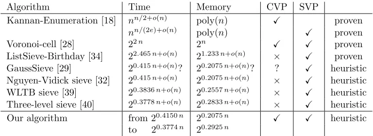
Table 1: Complexity of currently known SVP/CVP algorithms.
Algorithm Time Memory CVP SVP
Kannan-Enumeration [18] nn/2+o(n) poly(n)
X proven
nn/(2e)+o(n) poly(n)
X proven Voronoi-cell [28] 22n 2n
X X proven
ListSieve-Birthday [34] 22.465n+o(n) 21.233n+o(n)
× X proven
GaussSieve [29] 20.415n+o(n)? 20.2075n+o(n)? ? X heuristic Nguyen-Vidick sieve [32] 20.415n+o(n) 20.2075n+o(n)
× X heuristic WLTB sieve [39] 20.3836n+o(n) 20.2557n+o(n)
× X heuristic Three-level sieve [40] 20.3778n+o(n) 20.2833n+o(n) × X heuristic Our algorithm from 20.4150n 20.2075n X X heuristic
to 20.3774n 20.2925n
memory. Aclosest vector can be found by enumeration and by the Voronoi-cell algorithm, however, to the best of our knowledge, no sieve algorithm is known to provably solve CVP instances, and it would be interesting to study other sieve algorithms which also work in the CVP case. Table 1 presents the complexities of currently known SVP and CVP algorithms including our new algorithm. In particular, it shows that the asymptotic time complexity of our new approach (slightly) outperforms the complexity of the best pre-existing sieving algorithm and that, as a bonus, it can for the same price serve as a CVP algorithm. The high memory requirement limits the size of accessible dimensions, for example we need 3 TB of storage in dimension 90 which we divide into 25 groups of 120 GB in RAM, and we would need the double in dimension 96. For this reason, the algorithm, as well as other classical sieving techniques, is in practice not competitive with the fastest memoryless methods such as pruned enumeration or aborted BKZ. However, our experiments suggest that despite the higher memory requirements, the sequential running time of our algorithm is of the same order of magnitude as the Gauss sieve, but with an easier to parallelize algorithm.
A long standing open question was to find ways to decrease the complexity of enumeration-based algorithms to a single exponential time complexity. On an LLL- or BKZ-reduced basis [24, 37] the running time of Schnorr-Euchner’s enumeration is doubly exponential in the dimension. If we further reduce the basis to an HKZ-reduced basis [23], the complexity becomes 2O(nlogn)[21, 18]. Enumeration
would become simply exponential if a quasi-orthonormal basis, as defined in Sect. 2, could be found. Unfortunately, most lattices do not possess such a favorable quasi-orthonormal basis. Also for random lattices the lower bound on the Rankin invariant is of size 2Θ(nlogn) and determines the minimal complexity for enumeration that operates exclusively on the original lattice. We provide a more detailed discussion in Sect. 2.
Our approach circumvents this problem by making use of overlattices that admit a quasi-orthonormal basis. These overlattices are found in polynomial time by an algorithm relying on the structural reduc-tion introduced by [14], as described in Sect. 3.3. Once we have an overlattice and its quasi-orthonormal basis, we may efficiently enumerate short vectors at a constant factor of the first minimum in the over-lattice. Our main task is to turn these small samples into a solution vector in the initial over-lattice. The construction is very similar to an observation by Mordell [31] in 1935 which presented the first algo-rithmic proof of Minkowski’s inequality using only finite elements. Namely, he observed that given a latticeLi and an overlatticeLi+1 ⊃ Li such that [Li+1 : Li] =r, in any pool of at leastr+ 1 short
vectors ofLi+1, there exist at least two vectors whose difference is a short non-zero vector inLi. This
lattice by a concrete, albeit exponential-time, algorithm.
The new algorithm solves SVP and CVP for random lattices in the spirit of a sieving algorithm, except that intermediate vectors lie in overlattices or cosets of overlattices whose geometry vary from dense lattices to quasi-orthogonal lattices. Alternatively, the algorithm can be viewed as an adaptation of the representation technique that solves knapsack problems [4] and decoding problems [25, 5] to the domain of lattices. Due to the richer structure of lattices, the adaptation is far from straightforward. To give a brief analogy, instead of searching for a knapsack solution, assume that we want to find a short vector in an integer lattice. An upper-bound on the Euclidean norm of the solution vector provides a geometric constraint, which induces a very large search space. The short vector we seek can be decomposed in many ways as the sum of two shorter vectors with integer coefficients. Assuming that these sums provideN different representations of the same solution vector, we can then choose any arbitrary constraint which eliminates all but a fraction ≈1/N of all representations. With this additional constraint, the solution vector can still be efficiently found, in a search space reduced by a factorN. From a broader perspective, this technique can be used to transform a problem with a hard geometric constraint, like short lattice vectors, into an easier subproblem, like short integer vectors (because Zn has an orthonormal basis), together with a custom additional constraint, which is in
general linear or modular, which allow an efficient recombination of the solutions to the subproblems. The biggest challenge is to bootstrap the algorithm by finding suitable and easier subproblems using overlattices. We propose a method that achieves this thanks to a well-chosen overlattice allowing an efficient deterministic enumeration of vectors of bounded norm. In this way, we can compute a starting set of vectors that is used to initiate a sequence of recombinations that ends up solving the initially considered problem.
Our contribution: We present a new heuristic algorithm for the exact SVP and CVP for n-dimensional lattices using a tower of k overlattices Li, where L = L0 ⊆ .. ⊆ Lk. In this tower,
we choose the lattice Lk at the bottom of the tower in a way that ensures that we can efficiently
compute a sufficiently large pool of very short vectors inLk. Starting from this pool of short vectors,
we move from each lattice of our tower to the one above usingsummationof vectors while controlling the growth of norms.
For random lattices and under heuristic assumptions, twoLi+1-vectors sum up to anLi-vector with
probability α1n, where vol (Li)/vol (Li+1) = αn > 1. We allow the norm to increase by a moderate
factorαin each step, in order to preserve the size of our pool of available vectors per lattice in our tower.
Our method can be used to find vectors of bounded norm in a latticeLor, alternatively, in a coset x+L,x ∈ L/ . Thus, in contrast to classical sieving techniques, it allows us to solve both SVP or CVP, and more generally, to enumerate all lattice points within a ball of fixed radius. The average running time in the asymptotic case is 20.3774n, requiring a memory of 20.2925n. It is also possible to choose different time-memory tradeoffs and devise slower algorithms that need less memory. We report our experiments on random lattices and SVP challenges of dimension 40 to 90, whose results confirm our theoretical analysis and show that the algorithm works well in practice. We also study various options to parallelize the algorithm and show that parallelization works well on a wide range of computer architectures.
2
Background and notation
Lattices and cosets. A lattice L of dimension n is a discrete subgroup of Rm than spans an
n-dimensional linear subspace. A lattice can be described as the set of all integer combinations
{Pni=1αibi|αi ∈ Z} of n linearly independent vectors bi of Rm. Such vectors b1, ..,bn are called
a basis of L. The volume of the lattice L is the volume of span(L)/L, and can be computed as
p
which can be upper bounded by Minkowski’s theorem asλ1(L)≤√nvol (L) 1/n
. We call acoset ofL a translationx+L={x+v|v∈ L}ofLby a vectorx∈span(L).
Overlattice and index. A latticeL0 of dimensionnsuch thatL ⊆ L0 is called an overlattice ofL. The quotient groupL0/L is a finite abelian group of order vol(L)/vol(L0) = [L0:L].
Hyperballs. Let Balln(R) denote the ball of radius R in dimension n where we omit n if it is
implied by the context. The volumeVn of then-dimensional ball of radius 1 and the radiusrn of the
n-dimensional ball of volume 1 are respectively:
Vn =
√πn
Γ n2 + 1 andrn=V
−1/n
n =
r
n
2πe(1 +o(1)).
Gaussian heuristic. In many cases, when we wish to estimate the number of lattice points in a “nice enough” setS, we can use the Gaussian heuristic. In this paper, we will quantify the Gaussian
Heuristic as follows:
Heuristic 2.1 ((Gaussian Heuristic)) There exists a constant2GH≥1such that for all the lattices
Land all the sets S that we consider in this paper, the number of points in S∩ Lsatisfies:
1 GH ·
vol(S)
vol(L) ≤#(S∩ L)≤GH·
vol(S)
vol(L) .
In fact, it can be proved that for any bounded measurable set S, the expectation, over random unit volume lattices drawn from the Haar distribution [2], of the number of non-zero points is always the volume of S. Also, for any fixed lattice of unit volume and any fixed bounded measurable set S, the expectation of the number of lattice points int+S for uniform tmoduloL is exactly vol(S). However, fewer results are known about the the standard deviation, or whether these distributions are concentrated enough around the expectation so that almost all instances satisfy the upper and lower bounds.
In this paper, the geometry of lattices vary between random integer lattices of large enough volume and quasi-orthonormal lattices. We will assume that in these lattices, the length λ1 of the shortest
vector is the one given by the Gaussian heuristic, i.e. the radius of a ball of volume vol (L): λ1(L)≈
rn· n p
vol (L).Furthermore, the setsS we consider in this paper are either balls of radius larger than
p
3/2rn n p
vol (L), and whose center is uniform modulo the lattice (i.e. far from0), or the intersection of two of such balls whose centers are close enough. In these cases, our experiments indicate that the number of lattice points in these sets are almost always between 50% and 110% of vol (S)/vol (L), thus Heuristic 2.1 holds in practice forGH= 2.
Gram-Schmidt orthogonalization (GSO). The GSO of a non-singular square matrix B is the unique decomposition as B = µ·B∗, where µ is a lower triangular matrix with unit diagonal and B∗ consist of mutually orthogonal rows. For eachi∈[1, n], we call πi the orthogonal projection over
span(b1, ..,bi−1)⊥. In particular, one hasπi(bi) =b∗i, which is thei-th row ofB∗. We use the notation
B[i,j] for the projected block [πi(bi), . . . , πi(bj)].
Rankin factor and quasi-orthonormal basis. Let B be an n dimensional basis of a lattice L, andj≤n. We call the ratio
γn,j(B) =
vol(B[1,j])
vol(L)j/n =
vol(L)(n−j)/n vol(πj+1(L))
2The algorithms and proofs would also work withG
the Rankin factor of B with index j. The well known Rankin invariants of the lattice, γn,j(L),
introduced by Rankin [35] are simply the squares of the minimal Rankin factors of index j over all bases ofL. This allows to define aquasi-orthonormal basis.
Definition 2.2 ((quasi-orthonormal basis)) A basis B is quasi-orthonormal if and only if its Rankin factors satisfy1≤γn,j(B)≤nfor allj∈[1, n].
In the above definition, we chose the upper-boundnover a generalpoly(n) only because we are able to achieve this factor. More generally, any polynomial function would be sufficient for the asymptotical analysis and for the running time. For example, any real triangular matrix with identical diagonal coefficients forms a quasi-orthogonal basis. More generally, any basis whosekb∗ik are almost equal is quasi-orthogonal. This is a very strong notion of reduction, since average LLL-reduced or BKZ-reduced bases only achieve a 2O(n2)
Rankin factor and HKZ-reduced bases of random lattices have a 2O(nlogn)
Rankin factor. Finally, Rankin’s invariants are lower-bounded [6, 38, 13] by 2Θ(nlogn) for almost all
lattices3, which means that only lattices in a tiny subclass possess a quasi-orthonormal basis.
Schnorr-Euchner enumeration Given a basisB of an integer latticeL ⊆Rn, Schnorr-Euchner’s
enumeration algorithm [37] allows to enumerate all vectors of Euclidean norm ≤ R in the bounded cosetC= (z+L)∩Balln(R) wherez∈Rn. The running time of this algorithm is
TSE= n X
i=1
# (πn+1−i(z+L)∩Balli(R)) , (1)
which is equivalent to
TSE≈ n X
i=1
vol(Balli(R))
vol(πn+1−i(L))
(2)
under Heuristic 2.1. The last term in the sums (1) and (2) denotes the number of solutions #C. Thus, the complexity of enumeration is approximately TSE≈O˜(#C)· max
j∈[1,n]
γn,j(B). This is why
a reduced basis of smallest Rankin factor is favorable. The lower bound on Rankin’s invariant of γn,n/2(L) = 2Θ(nlogn) for most lattices therefore determines the minimal complexity of enumeration
that is achievable while working with the original lattice, provided that one can actually compute a basis ofL minimizing the Rankin factors, which is also NP-hard. If the input basis is quasi-orthonormal, the upper-boundγn,j(B)≤nfrom Definition 2.2 implies that the enumeration algorithm runs in time
˜
O(#C), which is optimal. Without knowledge of a good basis one can aim to decompose the problem into more favorable cases that finally allow to apply Schnorr-Euchner’s algorithm as we describe in the following.
3
Enumeration of short vectors by intersection of hyperballs
The section presents the new algorithm that enumerates βn shortest vectors in any coset t+L of a lattice L for a constant β ≈ p3/2. It can be used to solve the NP-hard problems SVP, CVP, ApproxSVPβ and ApproxCVPβ: Given a lattice L, the SVP can be reduced to enumerating vectors of Euclidean normO(λ1(L)) in the coset0+L while a CVP instance can be solved by enumerating
vectors of norm at most dist(t,L) in the coset −t+L. These bounded cosets, (t+L)∩Balln(R) for
suitable radiusR, can be constructed in an iterative way by use of overlattices. The searched vectors are expressed as a sum of short vectors of suitable translated overlattices of smaller volume. The search for a unique element in a lattice as required in the SVP or CVP is delegated to the problem of enumerating bounded cosets. Any non-trivial element found by our algorithm is naturally a solution to the corresponding ApproxSVPβ or ApproxCVPβ.
3γ2
We present the new algorithm solving lattice problems based on intersections of hyperballs in Sec-tion 3.1 and the generic initializaSec-tion of our algorithm as described in SecSec-tion 3.3. Finally, SecSec-tion 3.4 describes the cost of the first step in the algorihtm.
3.1
General description of the new algorithm
Assume that we are given a tower ofk=O(n) latticesLi⊂Rn of dimensionnwhereLi⊆ Li+1 and
the volume of any two consecutive lattices differs by a factorN =dαn
e ∈N>1. We also assume that
the bottom latticeLk permits an efficient enumeration of theβn shortest vectors in any cosett+Lk
for 1< β <p3/2. The ultimate goal is to find theβn shortest vectors in some coset t
0+L0 ofL0.
We postpone how to find suitable latticesLi,i≥1, to the following two sections.
We also assume in this section, that the Gaussian heuristic (Heuristic 1) holds. Under this as-sumption, the problem of finding theβn shortest elements in some coset t+
L is roughly equivalent to enumerating all lattice vectors ofLin the ball of radiusβ·rn· n
p
vol (L) centered at−t∈Rn.
Each step fori=k−1 downto 0 of the algorithm is based on the following intuition: We are given the≈ βn shortest vectors vj in ti/2 +Li+1. By summation, we can then find vectors (vj+vl)j≤l
that lie inti+Li+1. We select those who actually lie inti+Li and whose norm is small enough, and
consider them as the input pool for the next step. For suitable parameters, namely αsmall enough andβ large enough, we thus recover the≈βn shortest vectors ofti+Li.
More precisely, for each i ∈[0, k], we callCi the bounded coset Ci that contains the βn shortest
vectors of the cosetti+Li whereti =t0/2i∈Rn. More formally, let us define
Ri=β·rnn p
vol(Li) andCi= (ti+Li)∩Ball(0, Ri)
such that
#Ci ≈vol(Ball(Ri))/vol(Li) =βn ,
which follows from the Heuristic 2.1. In addition, we recall that
Li⊂ Li+1 where vol(Li)/vol(Li+1) =dαne .
In order to enumerate C0, our algorithm successively enumerates Ci, starting fromi=k down to
zero, Figure 1 illustrates the sequence of enumerated lists.
C0
Ci
EnumerateCk
+ check (3),(4)
+ check (3),(4)
Figure 1: Iterative creation of lists.
z x
I z−x
Figure 2: Vector z ∈ Ci−1 found as sum
be-tweenx∈Ciandz−x∈Ci⇔I∩(ti+Li)6=
∅.
During the construction of the tower of lattices, which is studied in the next sections, we already ensure thatCk is easy to obtain. We now explain how we can computeCi−1 fromCi. To do this, we
compute all sumsx+y of vector pairs ofCi×Ci which satisfy the conditions
x+y∈ti−1+Li−1and (3)
kx+yk ≤β·rn· n p
This means that we collect theβn shortest vectors of the cosetC
i−1=ti−1+Li−1 by going through
Ci = ti+Li. In practice, an equivalent way to check if condition (3) holds, is to use an efficient
computation for the map ϕi−1 :Ci→ Li/Li−1,z→z−ti modLi−1 and to verify thatϕi−1(x) +
ϕi−1(y) = 0. Algorithm 1 summarizes our approach.
Algorithm 1Coset enumeration
Constants: α≈p4/3, β≈p3/2 Parameters: k
Input: A LLL-reduced basisB ofL0 and a centert∈Rn
Output: Elements oft+L0 of norm≤R0=βrnvol(L0)1/n
1: Randomize the input target by samplingt0∈t+L. Use for example a Discrete Gaussian
Distri-bution of parameter√nkB∗k. This defines all the sub-targetsti=t0/2i
2: Compute a tower of latticesL0, ..,Lk by use of Alg. 3 such that
-L0⊂ L1⊂...⊂ Lk and vol(Li)/vol(Li−1) =N =dαne
- lattice enumeration is easy onLk
- testing-morphismsϕi−1 fromti+Li toLi/Li−1 are efficient to evaluate.
3: Enumerate bottom cosetCk (with Schnorr-Euchner)
4: fori=k−1 downto 0 do
5: Ci←Merge(Ci+1, ϕi, Ri=βrnvol(Li)1/n) (Alg. 2)
6: end for 7: returnC0
A naive implementation of the merge routine that createsCi−1fromCi would just run through the
β2n pairs of vectors fromC
i×Ci, and eliminate those that do not satisfy the constraints (3) and (4).
By regrouping the elements ofCiintoαn buckets, according to their value moduloLi−1, condition (3)
implies that each element of Ci only needs to be paired with the elements of a single bucket, see
Algorithm 2. Heuristic 2.1 implies that each bucket contains at mostGH(β/α)n elements, therefore
the merge operation can then be performed in timeG2 H β2/α
n
.
Algorithm 2Merge by collision
/∗ Efficiently find pairs of vectors ofCi+1 s.t. their sum is in Ci ∗/
/∗ Ci denotes (ti+Li)∩Ball(Ri) ∗/
Input: The bounded cosetCi+1, a testing morphism ϕi and a radiusRi
Output: The bounded cosetCi
1: Ci← ∅
2: ReorganizeCi+1 into buckets indexed by the values ofϕi
3: for eachv∈Ci+1 do
4: for eachuin the bucket of index−ϕi(v)do
5: if ku+vk ≤Ri then
6: Ci←Ci∪ {u+v}
7: end if 8: end for 9: end for 10: returnCi
Complexity and constraints for parametersα and β. We now prove the complexity and cor-rectness of Algorithm 2.
Theorem 3.1 Assuming Heuristic 2.1, and provided thatβn
≥GH√n/0.692 p
1−α2/4n, then: Given
as input the bounded cosetCi+1, Alg. 2 outputs the cosetCi within G2H(β2/α)n Euclidean norm
20.375n
20.38n
20.385n
20.39n
20.395n
20.4n
20.405n
20.41n
20.415n
20.2n 20.21n 20.22n 20.23n 20.24n 20.25n 20.26n 20.27n 20.28n 20.29n 20.3n
ti
m
e
=
β
2 α
n
memory=βn
time vs. memory
α≈1, β=q43
α=q43, β=q32
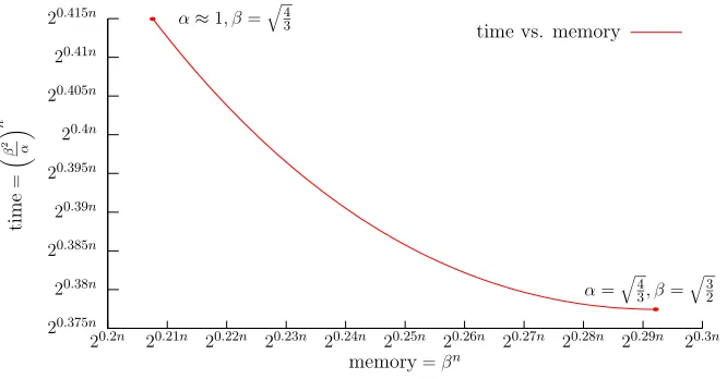
Figure 3: Trade-off between memory and time for varying choices ofαandβ.
Proof: It is clear that at each level, conditions (3) and (4) imply that Alg. 2 outputs a subset ofCi.
We now need to prove that there exist constantsαandβ such that all points ofCi are present in the
output. Equivalently, all points ofCi must be expressed as the sum of two points in Ci+1, see Fig. 2
for an illustration. This geometric constraint can be simply rephrased as follows: a vector z ∈ Ci
is found if and only if there exists at least one vectorx of the coset ti+1+Li+1 in the intersection
of two balls of radius Ri+1, the first one centered in 0, and the second one in z. It is clear that
z−x ∈ Ci+1 = ti+1 +Li+1 since 2ti+1 = ti and Li ⊆ Li+1. So if there is a point x ∈ Ci+1 in
the intersectionI = Ball(0, Ri+1)∩Ball(z, Ri+1), we obtain z ∈Ci as a sum between x∈Ci+1 and
z−x ∈ Ci+1. Under Heuristic 2.1, this occurs as soon as the intersection I of the two balls has a
volume larger thanGHvol(Li+1). We thus require that vol (I)/vol (Li+1)≥GH.
From Lemma A.1 and its corollary in the appendix, we derive that the intersection of two balls of radiusRi at distance at most Ri−1 =αRi is larger than 0.692·vol(Ball(Ri·
p
1−(α/2)2))/√n. A
sufficient condition onαandβ is then
β·p1−(α/2)2n≥G
H√n/0.692 or alternatively (5)
βp1−(α/2)2≥(1 +ε
n) (6)
whereεn= (GH√n/0.692)1/n−1 decreases towards 0 whenngrows.
Of course, for optimization reasons, we want to minimize the size of the listsβn, and the number
of steps (β2/α)n in the merge. Therefore we want to minimize β and maximizeα under the above
constraint. The total running time of Alg. 1 is given by B+ poly(n) β2/αn where
B represents the running time of the initial enumeration at levelk(details in Sect. 3.4). For optimal parameters, inequality (6) is in fact an equality. Asymptotically, the shortest running time occurs forα=p4/3 and β=p3/2 for which a merge costs around (β2/α)n
≈20.3774nand the size of the lists isβn
≈20.2925n.
3.2
Example for co-cyclic lattices or
q
-ary lattices.
We now give a simple intuition on how we could define the overlattice tower in the case of random co-cyclic lattices and q-ary lattices. These examples help to understand the idea that even for hard lattices, it is fairly easy to find quasi-orthonormal bases in overlattices. In the next section, we will present a more general method to create randomized overlattices, which performs well in practice for all types of lattices, including cocyclic orq-ary lattices, and ensures the estimated complexity as denoted in Sect. 3.1 which is based on Heuristic 2.1.
In the following description, the tower of lattices remains implicit in the sense that we do not need to find a basis for each of thek+ 1 latticesLi. We only need a description of the initial and the bottom
lattice as we test membership to a coset by evaluatingϕi.
LetL ⊆ Zn be a co-cyclic lattice given as
L ={x∈ Zn,Pn
i=1aixi = 0 modM} for large M ∈ N
and random integersa1, .., an ∈[0, M −1]. The task is to enumerateC = (t+L) ∩ Balln(R) where
R = β·rn·vol(L)1/n for a given β > 1. For k = O(n), the connection with random subset sum
instances, as well as newer adaptations of worst-case to average case proofs (see [14]) support the claim that random instances are hard. Chooseαsuch thatM =αnk
∈Nand defineN=αn∈N. We
can naturally define the tower consisting of lattices
Li={y∈Zn, n X
i=1
aiyi= 0 modNk−i} .
At the level k, we have Lk = Zn so that we can efficiently enumerate any coset C by use of the
Schnorr-Euchner algorithm [37] in timepoly(n)· |C|as we argue in Sect. 2. The coset testing function ϕi, which representsx−ti modLi−1, can be implemented asha,x−tii/Nk−i modN.
A second example is the class ofq-ary lattices. LetL be the lattice of dimensionnand volumeqk such that forx∈Zn,
x∈ L ⇐⇒ [(a1,1x1+..+a1,nxn≡q 0)∧..∧(ak,1x1+..+ak,nxn≡q0)] (7)
where ai,j are uniform in Z/qZ. Forq =αn classical worst-case to average-case reductions prove
that these lattices provide difficult lattice problems on average [1]. Here, a latticeLicould be defined as
the lattice satisfying the lastiequations of (7). Again,LkisZn,Li−1⊆ Liand vol (Li−1)/vol (Li) =q.
The coset testing functionϕi can be computed ashai,x−tii modq.
As elegant as it may seem, these simple towers of lattices are not as efficient as one could expect, because the top overlattice is Zn, and the Gaussian heuristic does not apply to its bounded coset
Ck =Zn∩Balln(Rk), whose radiusRk is too close to√n. Indeed, the number of points ofZn in a ball
of radiusRk ≈√nvaries by exponential factors depending on the center of the ball [26]. If the target
is very close to 0, like in an SVP-setting, the cosetCk contains around 20.513n vectors4, which differs
considerably fromβn ≈20.292n that we could expect of a random lattice. The initial coset would be very costly to store already in moderate dimensions.
Even if we store only a fraction of the bottom coset, Heuristic 2.1 would prevent the first merge by collision from working. Indeed, it relies on the number of points in intersections of balls of radius Rk centered in an exponential number of different points. Unfortunately, balls of radiusRk centered
in random points contain an exponentially smaller number of integer vectors thanβn, and their
inter-sections contain in general no integer point at all. Thus the collision by merge would fail to recover Ck−1.
This means that because of the Gaussian heuristic, the Zn lattice should never be used as the
starting point of an overlattice tower. Fortunately, random quasi-orthonormal lattices are a valid replacement ofZn, as our experiments show. Furthermore, we can still build in polynomial time a
tower of lattices ending with a quasi-orthonormal basis. We give the details of a generic generation of a tower of lattices in the following section.
4Computation based on saddle point method as in [26] for a radiusp
3.3
Generic creation of the tower
For any integer latticeL, the simplest choice of an overlattice isL0 =Zn. However, this creates two
problems.
1. Zn does not satisfy our quantified version of the Gaussian heuristic 2.1, as it would require an
n-exponentialGH.
2. The index [Zn : L], which is the volume of L might be too large. Indeed, our sieve requires
that the index is simply exponential but an integer basis with polynomial entries may have a superexponential volume 2poly(n).
For the first problem, it suffices to replace the square latticeZn by a quasi-orthogonal latticeL0.
Indeed, although the expectation of the number of lattice points in a randomly centered ball of radius rnβvol(L0)1/nis alwaysβn, their repartition is much more concentrated around the expectation when
the lattice is quasi-orthonormal than when it isZn. In practice, almost all of these balls contain at
leastβn/2 lattice points, and Heuristic 2.1 is valid with G
H = 2. The most noticeable exception is
when the center is too close to a lattice point. In this very rare case, the number of points would exceed the upper-bound by an exponential factor. Luckily, the lower-bound in Heuristic 2.1 is more important than the upper-bound: the lower-bound is used an exponential number of times in Eq. (5) to prove the correctness of the merge, whereas the upper-bound is used only with a polynomial number of different centers, to obtain the time and memory complexities. Thus bad centers are easy to avoid. For the second problem, one can see that the difficulty of creating the sieve is not just to find a quasi-orthonormal overlattice (which is always possible), the difficulty is to find one of small index. That is why we need a several overlattices instead of just one.
We now present a generic method of computing the tower of Li’s that works well in practice for
high dimensions as we have verified in our experiments. Algorithm 3 summarizes the following steps. We take as input a randomized LLL-reduced or BKZ-30-reduced basisBof ann-dimensional lattice
L. We choose constants α >1 andβ >0 satisfying equation (6) with the additional constraint that N=αn is an integer.
The Gram-Schmidt coefficients of B usually decrease geometrically, and we can safely assume that minikb∗ik ≥ maxikb∗ik/
p
4/3n. Otherwise, the LLL-reduced basis would immediately reveal a sublattice of dimension < n containing the shortest vectors of L. This means that there exists a smallest integerk=O(n) such that mini∈[1,n]kb∗ik ≥
vol(L) Nk
1
n
=σ. The integerk determines the
number of levels in our tower andσis then-th root of the volume of the last overlatticeLk.
Algorithm 3Compute the tower of overlattices
Input: B a (randomized) LLL-reduced basis ofL of dimensionn Output: BasesB(i) of a tower of overlattices
L=L0 ⊂ · · · ⊂ Lk. Note that given a targetti+1, the
testing morphismϕi fromti+1+Li+1toZN is implicitely defined byϕi
ti+1+P n j=1µjb
(i+1) j
=
µ1 modN
1: LetN =dαn
e.
2: Letkbe the smallest integer s.t. Nk
≥vol(L)/mini kb∗ikn.
3: Letσ= (vol(L)/Nk)1
n, thusσ≤mini kb∗ik.
4: Apply Alg. 4 on input (B, σ) to find a basis ˆB = [ˆb1,bˆ2. . . ,ˆbn] ofL.
5: B(i)
←hˆb1
Ni,ˆb2, . . . ,ˆbn i
foreachi∈[0, k]
6: returnB(i)for alli
It remains to find the tower (Li)i∈[1,k] of overlattices ofL, together with a quasi-orthonormal basis
B(k)of
Lk, given a structural conditionL(i)/L(i−1)'Z/NZ(Alg. 3). This problem is closely related
¯
Lsuch that ¯L/Lis isomporphic to some fixed abelian groupG. However, the primary goal of [14] was to decrease the Gram-Schmidt norm of ¯B in order to sample a pool of Gaussian overlattice vectors of norm Θ(√nlognkB¯∗k). These vectors would be too large for our purpose, since the bottom level of our decomposition algorithm needs a pool of vectors of length Θ(√npn vol( ¯
L)).
In the present paper, we prove that when the group Gis large enough, the unbalanced reduction
of [14] can in fact efficienlty construct a basisCofLsuch that [c1/Nk,c2, . . . ,cn] is quasi-orthonormal.
This naturally defines the tower ofk+ 1 overlatticesLi, whereLi is generated by the corresponding
basis B(i) = [c1
Ni,c2, . . . ,cn] for i = 0, .., k. Then, the Gaussian sampling algorithm on Lk can be
replaced by Schnorr-Euchner’s enumeration – with or without pruning – using B(k), and thus, the
norm of the overlattice vectors can be decreased to rnβn p
vol(Lk). For completeness, we recall in
Appendix the pseudo-code of the unbalanced reduction from [14]. Here, we prove that it allows to produce a quasi-orthonormal basis. Compared to [14], we added the condition thatσ≤minkb∗ik on the input parameters, and consequently, one of the test cases in the main loop of the algorithm in [14] never occurs.
Theorem 3.2 and its corollary below prove that running the unbalanced reduction with a smaller parameterσthan what is considered in [14] allows to construct a quasi-orthonormal overlattice basis in polynomial time. Note that in [14], the goal was to find an overlattice basis whose Gram-Schmidt length was smaller thanσ without any constraints on their Rankin factors. Here, the first vector of the overlattice basis may be larger thanσ, we just ensure that then-th root of the volume is exactlyσ and that all Rankin factors are polynomially bounded. Thus, the main Equation (10) of Theorem 3.2 cannot be directly deduced from [14], and we provide a full proof in the appendix.5
Theorem 3.2 ((Unbalanced reduction)) Let L(B) be an n-dimensional integer lattice with an LLL-reduced basis B = [b1, .., bn]. Let σ be a target length ≤ minkb∗ik. Algorithm 4 outputs in
polynomial time a basisC ofL satisfying
kc∗ik ≤σfor alli∈[2, n] (8)
kc1k ≤σn·vol(L)/σn (9)
σn+1−i
vol(C[i,n]) ≤
n+ 1−ifor alli∈[2, n] (10)
Since σ is by construction the n-th root of the bottom lattice Lk, we immediately deduce the
following elementary corollary, which proves that Algorithm 3 computes a tower of overlattices suitable for the decomposition algorithm.
Corollary 1 Given as input a LLL-reduced basis B of L such that maxkb∗ik/minkb ∗
ik ≤ 2O(n),
Algorithm 3 outputs a sequence of bases B(0), . . . , B(k) such that B(0) is a basis of
L,B(k) is
quasi-orthogonal, andL(B(i))/
L(B(i−1))
'Z/NZfor alli∈[1, k].
Proof: The condition maxkb∗ik/minkb∗ik ≤2O(n) ensures that the numberk of levels computed in
Step 2 is linear inn. Thus, σ computed in Step 3 is ≤ minkb∗ik. From the definition of B(k), we
deduce that vol(L(B(k)) = vol(
L)/Nk =σn, and for alli
≥2,B([i,nk)] = ˆB[i,n]. Thus, Eq. (10) proves
that the Rankin factorγn,i(B(k)) =σn−i/vol(B (k)
[i+1,n]) is≤n−i for alli∈[1, n−1].
The proofs of Theorem 3.2 and Alg. 4 are given in Appendix B.
3.4
Cost for initial enumeration at level
k
and pruning
The cost of a full enumeration of any bounded coset (z+Lk)∩Balln(rnβσ) at levelkis:
TSE= n X
i=1
vol(Balli(rnβσ))
volB[(nk+1) −i,n] ≤ n
n X
i=1
Vi·(rnβ)i= ˜O 20.398n
(11)
where for n → ∞ the maximal term in the sum, ∼
√ nβ √
i i
, appears for i = nβ2/e. It is of size
˜
O 20.398n because √eβ2/e
≈ 20.398n. Experiments show that the above estimate is close to what
we observe in practice as we present in Sect. 4. The number of steps in the full enumeration is an exponential factor<20.03n larger than the complexity of the merge. In practical dimensions
≤100, the actual running time of the full enumeration is already smaller than the time for the merge by collision in the consecutive steps, as elementary operations in the enumeration are faster than memory access and vector additions in the merge. However, more work must be done in large dimensions. For instance, a light pruning [15, 12] can be used to divide the running time of the initial enumeration by a small exponential factor of 20.03n, but it will only recover a subsetSk ⊆Ck. For instance, by use of
the linear bounding function of [15], it will recover a fraction 1/nof Ck, and since depthn+ 1−iin
the pruned enumeration only explores a subset of thei-dimensional ball of radius pi/nrnβσ instead
ofrnβσ, the running timeTSE provably decreases below
Tlin.prun.
SE ≤
n X
i=1
volBalli q
i nrnβσ
volB[(nk+1) −i,n] ≤ n
n X
i=1
Vi rn r
i nβ
!i
≈n2βn = ˜O 20.292n. (12)
Of course, there are lots of pruning trade-offs between Eqs. (11) and (12). This leads to a natural question on the stability of the algorithm, namely if the input of the merge at leveliis an incomplete subset Si+1 containing only a constant or polynomially small fraction ν of all elements of Ci+1, is
the merge algorithm still be able to retrieve the whole set Ci. Intuitively, under some reasonable
independence heuristics,β should then be increased so that the volume of each ball intersection grows by a factor 1/ν2. Thus condition (5) becomesβnp1
−(α/2)2n ≥√nG
H/0.692ν2. But on the other
hand,GH can now be decreased from some large enough constant downto almost 1, since the Gaussian
heuristic 2.1 only needs to be valid for a fraction ≥ν of all intersections of balls, in order to get a fraction ≥ ν of Ci in the output. Working with incomplete cosets also raises additional questions,
namely how likely are short elements to be present in the incomplete output coset, and can this probability be increased with randomization and standard repetition arguments.
In the next section, we address these questions in our experimental results which implicitly uses GH = 1 for efficiency reasons.
4
Experimental validation
In this section we present our experimental results of a C++-implementation of our Algorithm 1, presented in Section 3. We make use of the newNTL [16] and fplll [7] libraries as well as the Open MP [33] and GMP [11] library. We tested the algorithm on random lattices of dimensions up ton= 90 as input.
4.1
Overview
Tests in smaller and larger dimensions confirm the choice of parametersαandβthat we computed for the asymptotic case. We are hence able to enumerate vectors of a target cosetC0= (t0+L0)∩Ball(R0)
and in this way we solve SVP as well as CVP. Indeed, unlike classical sieving algorithm, short elements,
Thus, even though we might miss some elements of the target coset, we almost always solve the respective SVP or CVP. For instance, the algorithm finds the same shortest vectors as solutions for the SVP challenges published in [36]. The memory requirement and running time in the course of execution closely match our estimates and the intermediate helper latticesLi behave as predicted.
Besides the search for one smallest/closest vector, each run of the algorithm, with appropriate parameters, finds a non-negligible fraction of the whole bounded cosetC0. Repeating the search for
vectors in C0 several times on a randomized LLL-reduced basis will discover the complete bounded
coset. Our experiments reflect this behavior where we can use the Gaussian heuristic or Schnorr-Euchner enumeration to verify the proportion of recovered elements ofC0.
All these tasks can be performed by a single machine or independently by a cluster as a distributed computation.
4.2
Recovering
C
0in practice for smaller dimensions
For design reasons we have described an algorithm that produces the same number of elements per list in each iteration in order to find all ofC0. All lists contain #C0= # ((t0+L0)∩Balln(R0))≈(1+εn)nβn
elements on average whereεn can be neglected for very large dimensions, (see also (5)). For accessible
dimensions, we need to increase the radii of the balls slightly, by a small factor 1+εn, that compensates
for small variations from the heuristic estimate. We here present results for different valuesεn≤0.08
and dimensionn∈ {40,45,50,55,60}. The larger the dimension, the better Heuristic 2.1 holds, which means that εn can be chosen smaller, see (6). Figure 4 shows the relation between varying εn and
the fraction of found vectors of C0 for dimension n ∈ {40,45,50,55,60}. The optimal choice forεn
depends onnand the fraction ofC0we wish to enumerate.
0 0.1 0.2 0.3 0.4 0.5 0.6 0.7 0.8 0.9 1
0.03 0.04 0.05 0.06 0.07 0.08 0.09 0.1
fraction of found vectors
ε
n=60 n=55 n=50 n=45 n=40
Figure 4: Fraction of vectors inC0found for
vary-ingεn.
50000 100000 150000 200000 250000 300000 340000
0 10 20 30 40 50 60 70 80 90 100
number of distinct elements
number of repetitions
|C0|
experiment |C0| |C0|*(1-(1-p)r)
Figure 5: Success probability afterr repetitions, n= 50,p= 0.06.
4.3
Probability of success for randomized repetitions - example: small
di-mension
The success ratio of recovering all ofC0 rises with increasingn. We here present the case of smaller
dimensionsn={50,55}to show how it evolves.
Suppose that we want to enumerate 100% of a cosetC0 in dimension 50. According to Fig. 4, we
need to chooseεnat least 0.07, which results in lists of size (1 +εn)50β50≈29.4β50and a running time
(1 +εn)100(β2/α)50≈867.7 (β2/α)50 on average. An alternative, which is less memory consuming, is
to choose a smallerεn, and to run the algorithm several times on randomized input bases. For instance,
if one choosesε= 0.0535, one should expect to recoverp= 6% ofC0 per iteration on average. Then,
assuming that the recovered vectors are uniformly and independently distributed inC0, we expect to
find a fraction of 1−(1−p)rafter rrepetitions.
deviation) in comparison to the expected number of elementsC0·(1−(1−0.06)r). The experiments
match closely the estimate.
For a random lattice of dimensionn= 50 andε= 0.0535, the size of the cosetC0is roughly 342 000.
In our experiments, we found 164 662 vectors (48%) after 10 repetitions in which we randomized the basis. After 20 trials, we found 239 231 elements which corresponds to 70%, and after 70 trials, we found 337 016 elements (99% ofC0). We obtained the following results in dimensionn= 55. After 10
trials withε= 0.0535, we obtain 96.5% of the vectors ofC0which is significantly higher in comparison
to the 48% recovered after 10 trials in dimension 50.
0 10 20 30 40 50 60 70
22 23 24 25 26 27 28 29 30 31
occurence of vector for 100 bases
norm of the vector
Figure 6: Correlation of occurrence of vectors and their length.
0 2e+06 4e+06 6e+06 8e+06 1e+07 1.2e+07 1.4e+07
0 10 20 30 40 50
number of vectors tested
projection i = 1 to 55 experiment
heuristic
Figure 7: Comparison between the actual number of nodes during enumeration and the Gaussian heuristic predictions for dimension 55.
4.4
Shorter or closer vectors are easier to find
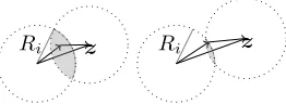
During the merge operations, we can find a vector v ∈ Ci if there exist vectors in the intersection
between two balls of the same radius, centered at the end points ofv. As the intersection is larger whenv is shorter, see Fig. 8, we can deduce that with the practical variant, short vectors of a coset are easier to find than longer ones.
Ri z Ri z
Figure 8: Volume of intersection varies for vectorsz of different length.
As we work with cosets, this means that vectors which are closer to the target (i.e., short lattice vectors when the target is 0) should appear more often for different runs on randomized input basis. We verified this observation experimentally by comparing the norm of a vector with the number of appearances during 100 repetitions in dimension 50, withε= 0.0535, see Fig. 6.
4.5
Parallelization
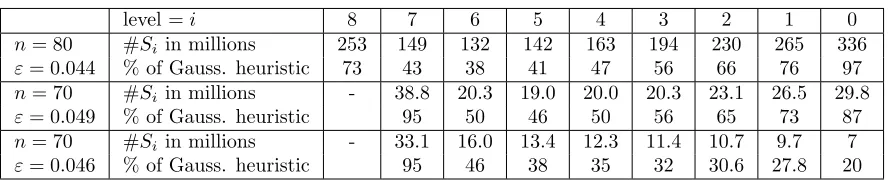
Table 2: Experimental results forn∈ {70,80}, α=p4/3 andβ =p3/2.
level =i 8 7 6 5 4 3 2 1 0
n= 80 #Si in millions 253 149 132 142 163 194 230 265 336
ε= 0.044 % of Gauss. heuristic 73 43 38 41 47 56 66 76 97 n= 70 #Si in millions - 38.8 20.3 19.0 20.0 20.3 23.1 26.5 29.8
ε= 0.049 % of Gauss. heuristic 95 50 46 50 56 65 73 87 n= 70 #Si in millions - 33.1 16.0 13.4 12.3 11.4 10.7 9.7 7
ε= 0.046 % of Gauss. heuristic 95 46 38 35 32 30.6 27.8 20
This allows to efficiently run the algorithm when the available RAM is too small to store lists of size (1 +ε)nβn. It also allows to distribute the merge step on a cluster. For instance, in dimensionn= 90
usingε= 0.0416, storing the full lists would require 3 TB of RAM. We divided the lists into 25 groups of 120 GB each, which we treated one at a time in RAM while the others were kept on hard drive. This did not produce any noticeable slowdown. Finally, the number of elements in each bucket can be estimated precisely in advance using Heuristic 2.1, and each group performs exactly the same vector operations (floating point addition, Euclidean norm computation) at the same time. This makes the algorithm suitable for SIMD implementation, not only multi-threading.
4.6
Experiments in low- and middle-sized dimensions
Our experiments in dimension 40 to 90 on challenges in [36] show that we find the same short vectors as previously reported and found as shortest vector by use of BKZ or sieving. To solve SVP or CVP by use of the decomposition technique, it is in fact not necessary to enumerate the complete bounded coset C0 and to ensure that the lists are always of size (1 +εn)nβn as we describe in the following
paragraphs.
We give more details for medium dimensionsn= 70 andn= 80 withα=p4/3 andβ=p3/2 in the following. The algorithm ran on a machine with an Opteron 6176 processor, containing 48 cores at 2.3 GHz, and having 256 GB of RAM. Table 2 presents the observed size of the listsSi ⊆Ci for
each level in dimension 70 and 80.
In dimension 80, we chose aborted-BKZ-30 [17] as a preprocessing. The algorithm has 8 levels and we choseε= 0.044 to obtain 97% of C0 after a single run. The initial enumeration on one core took
a very short time of 6.5 CPU hours (so less than 10 minutes with our multi-thread implementation of the enumeration) while each of the 8 levels of the merge took between 20 and 36 CPU hours (so less than 45 minutes per level in our parallel implementation).
The number of elements in lower levels lies below the heuristic estimate and we keep loosing elements during the merge for the deepest levels. For example, in dimension 80 we start with 73% ofC8 and
recover only 43% of C7 after one step. Towards higher levels, we slowly begin to recover more and
more elements. In dimension 80, the size of the lists starts to increase from level 5 on asS5, S4andS3
cover 41%, 47% and 56% of the vectors, respectively. This continues until the final step where we find 97% of the elements ofC0.
4.7
Pruning of the merge step in practice - larger dimension
n
= 75
and
n
= 90
In Section 3.1, we obtain conditions on the parameters as we request the intersectionI of two balls to be non-empty, which means that vol(I)/vol(L)≥K for some numberK >1 under Heuristic 2.1. This condition suggests that at each level, each coset element in an output listSi−1⊆Ci−1of a merge
is obtained on average aboutK times. If the input list Si is shorter than expected, one will indeed
recover fewer thanKcopies of each element, but we may still have one representative of each element ofCi−1. Our experiments confirm this fact, see Tab. 2 and Tab. 3. To solve SVP or CVP, one may
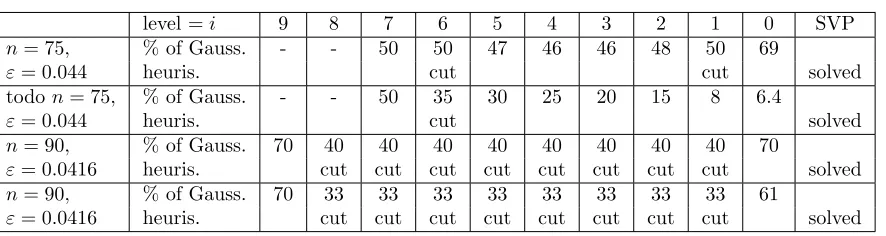
Table 3: Experimental resultswith pruning,n∈ {75,80,90}, α=p4/3 andβ=p3/2.
level =i 9 8 7 6 5 4 3 2 1 0 SVP
n= 75, % of Gauss. - - 50 50 47 46 46 48 50 69
ε= 0.044 heuris. cut cut solved
todon= 75, % of Gauss. - - 50 35 30 25 20 15 8 6.4
ε= 0.044 heuris. cut solved
n= 90, % of Gauss. 70 40 40 40 40 40 40 40 40 70
ε= 0.0416 heuris. cut cut cut cut cut cut cut cut solved n= 90, % of Gauss. 70 33 33 33 33 33 33 33 33 61
ε= 0.0416 heuris. cut cut cut cut cut cut cut cut solved
the output list contains a sufficiently large fraction of the elements of the bounded cosets. For example, we ran our algorithm on the 75-dimensional basis of the SVP challenge [36] with seed 38. We chose ε= 0.044 and interrupted the merge if the size of the intermediate setSi reached 50% or 35% of #Ci
fori∈[1, k−1]. Tab. 3 presents the intermediate list sizes. In the end, we recovered 69% and 6.4% of #C0, respectively, and the shortest vector was found in both cases. The running time for the merge
in the intermediate levels decreases compared to no pruning by a factor 0.49 and 0.29, respectively, as one would expect for lists that are smaller by at least a factor 0.5 and 0.35, respectively.
In dimension 90, we ran our algorithm on the 90 dimensional SVP-challenge with seed 11, using ε= 0.0416. We chose to keep at most 33% of Ci for i ∈[1, k−1]. Despite this harsh cut, the size
of the intermediate lists remained stable after the first merge. And interestingly, after only 65 hours on 32 threads, we recovered 61% of #C0 in the end, including the published shortest vector. Note
that as we interrupt the merge, we in fact do not read all elements of the starting listSk. One might
hence simply not apply a full enumeration in practice but stop the Schnorr-Euchner enumeration once enough elements are enumerated.
4.8
Notes on the Gaussian heuristic for intermediate levels
Our quasi-orthogonal lattices at the bottom level behave randomly and follow the Gaussian heuristic. The most basic method to fill the bottom listSk is to run Schnorr-Euchner enumeration (see Sect. 2)
where the expected number of nodes in the enumeration tree is given by (11) based on Heuristic 2.1. Previous research has established that this estimate is accurate for random BKZ-reduced bases of random lattices in high dimension. Here, since we work with quasi-orthogonal bases, which are very specific, we redo the experiments, and confirm the findings also for quasi-orthogonal bases. Already for small dimensions (n= 40,50,55), experiments show that the actual number of nodes in a Schnorr-Euchner enumeration is very close to the expected value. Figure 7 shows that experiment and heuristic estimate for dimension 55, for example, are almost indistinguishable.
We also make use of Heuristic 2.1 when we estimate the number of coset vectors in the intersection of two balls. As the lower lattices in the tower are not ”random” enough, they have close to quasi-orthonormal bases, we observe smaller lists in the lower levels and thus a deviation from the heuristic. Beside the geometry of lattices, the deviation depends on the center of the balls or the center of the intersection. Randomly centered cosets of quasi-orthonormal lattices contain experimentally an average number of points a constant factor below (1 +εn)nβn. Zero-centered cosets contain more points, and
should be avoided. The randomization of the initial target used in Alg. 1 ensures that the centers are random moduloLk, even in an SVP setting. The number of vectors stays hence below, but close to the
estimate (1 +εn)nβn after the first collision steps. The following steps can only improve the situation.
The lattices in higher levels are more and more random and we observe that the algorithm recovers the expected number of vectors. This is a sign that our algorithm is stable even when the input pools Si are incomplete.
α=p4/3, β=p3/2, ε= 0.044, we observe that the largest bucket contains only 10% more elements than the average value, and that 60% of the buckets are within±2% of the average value.
4.9
Comparison to experimental results of a parallel Gauss sieve algorithm
From a very general point of view, our algorithm can be viewed as a Sieving algorithm. The algorithm is decomposed into a polynomial number of levels, each one corresponds to a certain upper-boundRi
on the norm. At each level, we use an exponential pool of lattice vectors, perform linear combinations, and select the shortest of them for the next level.
We now list the specificities of our algorithm compared to previous sieving algorithms:
• We start from short vectors (in overlattices) and at each level, the normRigeometrically increases
by a factorα.
• At each level, we maintain an (almost) complete set of all coset vectors of norm≤Ri. For this
reason, our algorithm has the stability property that short coset vectors are more likely to be found. Classical sieving techniques satisfy the opposite: short vectors have a negligible property to appear spontaneously. Our algorithm is compatible with pruning, and it can solve the Exact CVP. Reducing the list sizes for classical sieving leads in general to catastrophic results.
• Our algorithm is highly parallelizable as it allows to use up toαn independent threads per merge operation as explained in Sect. 4.5. However the accessible dimension is naturally limited by the exponential memory requirement of order βn. There exists parallel versions of the Gauss
sieve [30, 19], which leads to faster practical running time in dimensions 70 to 96, however the efficiency of the parallelization decreases fast when the number of threads increases because of the list size and the communication cost [19].
• Our algorithm is essentially a CVP solver and is not specialized for SVP: if classical Sieving algorithms were to be turned into CVP solvers, then it would obviously be impossible to regroup each vector with its opposite, and the lists of vectors would be twice as large. Furthermore, classical Sieving techniques rely on the fact that vectors which cannot be reduced by others, necessarily become poles to reduce others. By replacing substractions with additions in order to preserve the target, these two options – can a vectorv be reduced by others vs. can−v be considered as a pole – cease to be mutually exclusive, and both would have to be tested. Thus, turning classical Sieving algorithms into CVP solvers would likely increase their running time by a factor 4 and their memory requirement by a factor 2, with no guarantee that they would actually find the solution.
We give some concrete timings: To solve instances in dimension 80 and 90, our algorithm takes more time than the currently fastest implementation of the Gauss sieve algorithm [19]. Ishiguro et al. report in [19] to solve the SVP challenge in dimension 80 in 29 sequential hours and an instance of dimension 96 in 6400 sequential hours. Our algorithm however needs 65 sequential hours in dimension 80 and 2080 hours in dimension 90. It is slower than the Gauss Sieve used as an SVP solver, yet, the slowdown factor remains smaller than 4, which would be expected (as a minimum) to turn it into a CVP solver.
5
Conclusion
References
[1] M. Ajtai. The shortest vector problem in L2 is NP-hard for randomized reductions (extended
abstract). In STOC’98, pages 10–19, 1998.
[2] M. Ajtai. Random lattices and a conjectured 0 - 1 law about their polynomial time computable properties. InFOCS, pages 733–742, 2002.
[3] M. Ajtai, R. Kumar, and D. Sivakumar. A sieve algorithm for the shortest lattice vector problem. InProc. 33rd STOC, pages 601–610, 2001.
[4] A. Becker, J.-S. Coron, and A. Joux. Improved generic algorithms for hard knapsacks. InProc. of Eurocrypt 2011, LNCS 6632, pages 364–385. Springer-Verlag, 2011.
[5] A. Becker, A. Joux, A. May, and A. Meurer. Decoding random binary linear codes in 2n/20: How
1 + 1 = 0 improves information set decoding. InEUROCRYPT, volume 7237 ofLecture Notes in Computer Science, pages 520–536. Springer, 2012.
[6] M. I. Boguslavsky. Radon transforms and packings.Discrete Applied Mathematics, 111(1-2):3–22, 2001.
[7] X. Cad´e, D. Pujol and D. Stehl´e. fplll 4.0.4, May 2013.
[8] D. Coppersmith. Finding a small root of a bivariate integer equation; factoring with high bits known. InEUROCRYPT, pages 178–189, 1996.
[9] D. Coppersmith. Finding a small root of a univariate modular equation. InEUROCRYPT, pages 155–165, 1996.
[10] I. Dinur, G. Kindler, and S. Safra. Approximating-cvp to within almost-polynomial factors is np-hard. In Proceedings of the 39th Annual Symposium on Foundations of Computer Science, FOCS ’98, pages 99–, Washington, DC, USA, 1998. IEEE Computer Society.
[11] T. G. et al. GNU multiple precision arithmetic library 5.1.3, September 2013. https://gmplib.org/.
[12] M. Fukase and K. Yamaguchi. Finding a very short lattice vector in the extended search space.
JIP, 20(3):785–795, 2012.
[13] N. Gama, N. Howgrave-Graham, H. Koy, and P. Q. Nguyen. Rankin’s constant and blockwise lattice reduction. In CRYPTO, pages 112–130, 2006.
[14] N. Gama, M. Izabachene, P. Q. Nguyen, and X. Xie. Structural lattice reduction: Generalized worst-case to average-case reductions. Eprint report 2014/283, 2014.
[15] N. Gama, P. Q. Nguyen, and O. Regev. Lattice enumeration using extreme pruning. In EURO-CRYPT, pages 257–278, 2010.
[16] N. Gama, J. van de Pol, and J. M. Schanck. Fork of V. Shoup’s number theory library NTL, with improved lattice functionalities. http://www.prism.uvsq.fr/~gama/newntl.html, Febru-ary 2013.
[17] G. Hanrot, X. Pujol, and D. Stehl´e. Analyzing blockwise lattice algorithms using dynamical systems. InCRYPTO, pages 447–464, 2011.
[19] T. Ishiguro, S. Kiyomoto, Y. Miyake, and T. Takagi. Parallel gauss sieve algorithm : Solving the svp in the ideal lattice of 128-dimensions. Cryptology ePrint Archive, Report 2013/388, 2013.
[20] A. Joux and J. Stern. Lattice reduction: A toolbox for the cryptanalyst.J. Cryptology, 11(3):161– 185, 1998.
[21] R. Kannan. Improved algorithms for integer programming and related lattice problems. In
Proceedings of the fifteenth annual ACM symposium on Theory of computing, STOC ’83, pages 193–206, New York, NY, USA, 1983. ACM.
[22] R. M. Karp. Reducibility among combinatorial problems. In R. E. Miller and J. W. Thatcher, editors, Complexity of Computer Computations, The IBM Research Symposia Series, pages 85– 103. Plenum Press, New York, 1972.
[23] A. Korkine and G. Zolotarev. Sur les formes quadratiques. Mathematische Annalen 6, pages 336–389, 1973.
[24] A. K. Lenstra, H. W. Lenstra, and L. Lov´asz. Factoring polynomials with rational coefficients.
Mathematische Annalen, 261:515–534, 1982.
[25] A. May, A. Meurer, and E. Thomae. Decoding random linear codes in 20.054n. InASIACRYPT,
pages 107–124, 2011.
[26] J. E. Mazo and A. M. Odlyzko. Lattice points in high-dimensional spheres. Monatshefte f¨ur Mathematik, 110:47–62, 1990.
[27] D. Micciancio. The shortest vector in a lattice is hard to approximate to within some constant. In Proceedings of the 39th Annual Symposium on Foundations of Computer Science, FOCS ’98, pages 92–, Washington, DC, USA, 1998. IEEE Computer Society.
[28] D. Micciancio and P. Voulgaris. A deterministic single exponential time algorithm for most lattice problems based on Voronoi cell computations. In Proceedings of the 42nd ACM symposium on Theory of computing, STOC ’10, pages 351–358, New York, NY, USA, 2010. ACM.
[29] D. Micciancio and P. Voulgaris. Faster exponential time algorithms for the shortest vector problem. InSODA, pages 1468–1480. ACM/SIAM, 2010.
[30] B. Milde and M. Schneider. A parallel implementation of gausssieve for the shortest vector problem in lattices. In PaCT, pages 452–458, 2011.
[31] L. J. Mordell. On some arithmetical results in the geometry of numbers.Compositio Mathematica, 1:248–253, 1935.
[32] P. Q. Nguyen and T. Vidick. Sieve algorithms for the shortest vector problem are practical. J. of Mathematical Cryptology, 2008.
[33] OpenMP Architecture Review Board. OpenMP API version 4.0, 2013.
[34] X. Pujol and D. Stehl´e. Solving the shortest lattice vector problem in time 22.465n. IACR
Cryp-tology ePrint Archive, 2009:605, 2009.
[35] R. Rankin. On positive definite quadratic forms. J. Lond. Math. Soc., 28:309–314, 1953.
[36] M. Schneider, N. Gama, P. Baumann, and P. Nobach. http://www.latticechallenge.org/svp-challenge/halloffame.php.
[38] J. L. Thunder. Higher-dimensional analogs of Hermite’s constant. Michigan Math. J., 45(2):301– 314, 1998.
[39] X. Wang, M. Liu, C. Tian, and J. Bi. Improved Nguyen-Vidick heuristic sieve algorithm for shortest vector problem. In Proceedings of the 6th ACM Symposium on Information, Computer and Communications Security, ASIACCS ’11, pages 1–9, New York, NY, USA, 2011. ACM.
[40] F. Zhang, Y. Pan, and G. Hu. A Three-Level Sieve Algorithm for the Shortest Vector Problem. In T. Lange, K. Lauter, and P. Lisonek, editors, SAC 2013 - 20th International Conference on Selected Areas in Cryptography, volume Lecture Notes in Computer Science, Burnaby, Canada, Aug. 2013. Springer.
A
Intersection of hyperballs
The volume of the intersection, volI(d), of twon-dimensional hyperballs of radius 1 at distance d∈
[0.817; 2] can be approximated for large n by the volume of the n- dimensional ball of radius D =
q
1− d22, see Lemma A.1 below. If we consider the intersection of two balls of radiusR, the volume gets multiplied by a factorRn as stated in Corollary 2.
Lemma A.1 The volume of the intersection of two n-dimensional hyperballs of radius 1 at distance
d∈[0.817; 2]is
2Vn−1
(n+ 1)Vn
arccos
d
2
≤vol(volBallI(d)
n(D))≤
2Vn−1
(n2 + 1)Vn
arccos
d
2
whereD=
q
1− d22.
Proof: The intersection of two balls of radius 1 whose centers are at distanced∈[0,2] of each other can be expressed as
volI(d) = 2· Z 1
d
2
Vn−1 p
1−x2n−1dx= 2V n−1
Z arccos(d/2)
0
sinn(θ)dθ
where Vn−1 equals the volume of the n−1-dimensional ball of radius 1. For d∈ [0.817; 2] one can
bound the sinus term in the integral:
D
arccos(d/2)θ ≤ sin(θ) ≤
D
p
arccos(d/2)
√
θ .
Therefore, we obtain bounds for the volume of the intersection:
volI(d)≤
2Vn−1 n 2 + 1
arccos
d
2
Dn
and
volI(d)≥
2Vn−1
n+ 1 arccos
d
2
Dn
which proves the lemma.
Corollary 2 For all dimensionsn≥10, the volume of the intersection of twon-dimensional hyperballs of radiusR at distancedR whered≤p4/3is lower-bounded by:
RnvolI(d)≥
0.692
√n ·Rnvol
Balln
s
1−
d 2
2
.
B
Proof of Theorem 3.2 and Algorithm 4:
Algorithm 4Unbalanced Reduction from [14], specialized forσ≤minkb∗ik
Input: A LLL-reduced basisB of an integer latticeL, and a target lengthσ≤minkb∗ik Output: A basisCofLsatisfyingkc1k ≤σnvol(L)/σn, and for alli∈[2, n],kc∗ik ≤σand
σn+1−i
vol(C[i,n]) ≤
n+ 1−i. 1: C←B
2: Compute the Gram-Schmidt matricesµandC∗ 3: Letkbe the largest index such thatkc∗kk> σ 4: fori=k−1, . . . ,1 do
5: γ←
&
−µi+1,i+ kc∗i+1k
kc∗
ik
rkc∗
ik
σ 2
−1
'
6: (ci,ci+1)←(ci+1+γ·ci,ci)
7: Update the Gram-Schmidt matricesµandC∗. 8: end for
9: returnC
We use the suffix “old” and “new” to denote the values of the variables at the beginning and at the end of the “for” loop of Alg. 4, respectively. Furthermore, we callxithe valuekb∗inewkduring iteration
i. Note thatxi is alsokb∗ioldk during the next iteration (of indexi−1 sincei goes backwards).
Fori∈[1, n], let ai =kbi∗k/σ. Note thatai is always≥1. We show by induction overithat the
following invariant holds at the end of each iteration of Alg. 4:
aixi+1≤xi≤aixi+1+σai . (13)
At the first iteration (i=k−1), it is clear thatxk=kb∗koldk=σak . At the beginning of iterationi,
we always havekb∗ioldk> σ, and by induction, kb∗i+1oldk> σ. We transform the block so that the norm of the first vector satisfies
R≤ kb∗inewk ≤R+kb∗ioldk (14) whereR=kb∗i+1oldkkb
∗old i k/σ .
This condition can always be fulfilled with a primitive vector of the formbnewi =boldi+1+γboldi for some γ∈Z. Since the volume is invariant, the newkb∗i+1newk is upper-bounded byσ. And by construction,
Equation (14) is equivalent to the invariant (13) sincekb∗ioldk=aiσ,kb∗inewk=xi andkb∗i+1oldk=xi+1.
By developping (13), we derive a bound onx1:
x1≤σ k X
i=1
a1. . . ai≤σn k Y
i=1
ai≤nσvol(L)/σn
to (10). Note that the transformation matrix of the unbalanced reduction algorithm is
γ1 · · · γk−1 1 0 · · · 0
1 0 · · · 0 ... ... 0 . .. . .. ... ... ... 0 0 1 0 0 · · · 0 0 · · · · · · 0 1 0 0
..
. ... 0 . .. 0 0 · · · · · · 0 0 0 1
whereγi is l
−µi+1,i+xiσ+1 q
1−a12
i
m
. Since each xi+1is bounded by
n Y
j=i+1
aj= n Y
j=i+1
max(1,||b∗j||2/σ) ,
all coefficients have a size polynomial in the input basis. This proves that Alg. 4 has polynomial
running time.
Anja Becker EPFL, ´Ecole Polytechnique F´ed´erale de Lausanne, Laboratory for cryptologic algorithms (LACAL),
Switzerland.
Nicolas Gama UVSQ/PRISM, Universit´e de Versailles, France. [email protected]
Antoine Joux CryptoExperts, INRIA/Ouragan,
Chaire de Cryptologie de la Fondation de l’UPMC,