A sp ects o f th e R elation sh ip
b etw een
A ctiv e R egions and
C oronal M ass E jection s
Lucinda Green
Milliard Space Science Laboratory
Department of Space and Climate Physics
University College London
A thesis submitted to the University of London
All rights reserved
INFORMATION TO ALL USERS
The quality of this reproduction is dependent upon the quality of the copy submitted.
In the unlikely event that the author did not send a complete manuscript and there are missing pages, these will be noted. Also, if material had to be removed,
a note will indicate the deletion.
uest.
ProQuest U642441
Published by ProQuest LLC(2015). Copyright of the Dissertation is held by the Author.
All rights reserved.
This work is protected against unauthorized copying under Title 17, United States Code. Microform Edition © ProQuest LLC.
ProQuest LLC
789 East Eisenhower Parkway P.O. Box 1346
C ontents
1 In tro d u ctio n 11
1.1 The Solar A tm o s p h e re ... 12
1.1.1 The P h o to s p h e r e ... 12
1.1.2 The C h ro m o sp h e re... 13
1.1.3 The C o r o n a ... 15
1.1.4 Emission P ro c e s s e s ... 16
1.2 Magnetic F i e l d s ... 18
1.2.1 Generation of Magnetic F lu x ... 18
1.2.2 Equations Governing the Magnetic Field and Solar Plasm a . . 21
1.2.3 Magnetic R econnection... 24
1.2.4 Magnetic H e lic ity ... 26
1.3 Active Regions ... 27
1.3.1 D e f in itio n ... 27
1.3.2 Topology of the Magnetic F i e l d ... 28
1.3.3 Active Region F l a r e s ... 29
1.4 Coronal Mass E jectio n s... 32
1.4.1 D e f in itio n ... 32
1.4.2 Coronal Mass Ejections and their Relationship to Active Re gion Flares - Historical Review ... 34
1.4.3 CME Launch M e c h a n ism s... 37
1.4.5 CMEs and H e lic ity ...42
2 In stru m en ta tio n 44 2.1 The Yohkoh S p a c e c ra ft... 44
2.1.1 Soft X -ray T e le sc o p e... 45
2.1.2 The Hard X-ray T e le sc o p e ... 49
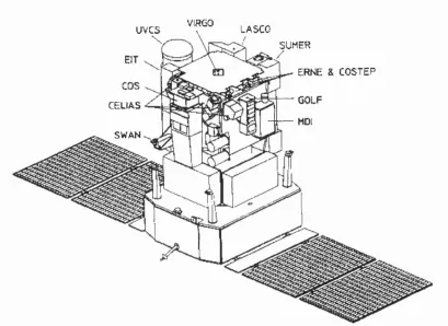
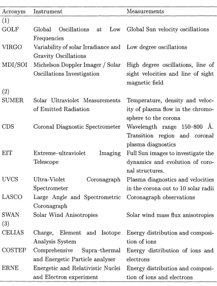
2.2 The Solar and Heliospheric Observatory ...51
2.2.1 The Extrem e-ultraviolet Imaging Telescope ... 55
2.2.2 The Large Angle and Spectroscopic C o r o n a g r a p h ... 59
2.2.3 The Solar Oscillations Investigation- Michelson Doppler Imager 65 2.3 Geostationary Operational Environmental S a te llite s ... 66
2.4 Ground Based In stru m e n ts ...67
3 Flare Survey 68 3.1 In tro d u c tio n ...68
3.2 Active Region S u rv e y ... 69
3.2.1 Active Region Selection ... 69
3.2.2 Identification of Coronal Mass Ejections ...70
3.2.3 Active Region F l a r i n g ... 73
3.2.4 Survey Results ...74
3.2.5 Flare Survey Discussion ... 79
3.3 NO A A Active Region 8 1 0 0 ...82
3.3.1 Flaring in Active Region 8100...83
3.3.2 D iscu ssio n ... 83
3.4 C o n c lu sio n s...86
4 H elicity E v o lu tio n in A c tiv e R egion 8100 89 4.1 In tro d u c tio n ...89
4.2 O bservations...94
C O N T E N T S 4
4.2.2 Evolution of the Photospheric Magnetic F i e l d ... 95
4.2.3 Evolution of the Coronal L o o p s ...100
4.2.4 The CME activity in Active Region 8 1 0 0 ... 100
4.3 Magnetic Helicity D e fin itio n ... 108
4.3.1 Helicity Injection by Differential Rotation ... 109
4.3.2 Coronal Magnetic H e lic ity ...112
4.3.3 Helicity lost through C M E s ... 114
4.3.4 D iscu ssio n ...118
4.4 C o n c lu sio n s... 122
5 O bservations o f a C onfined X I .2 Flare 125 5.1 In tro d u c tio n ... 125
5.2 Observations and A n a ly s is ...126
5.2.1 Coronagraph O b serv atio n s...126
5.2.2 Extrem e-Ultraviolet O b serv atio n s...129
5.2.3 Soft X -ray O b se rv a tio n s... 131
5.2.4 Hard X-ray O b servations...135
5.2.5 Evolution of the Photospheric f i e l d ... 137
5.3 D iscu ssio n ...140
5.4 C o n c lu sio n s... 144
6 C onclusions and Future R esearch 146 6.1 Flares and Coronal Mass ejectio n s...146
6.2 Active Region 8100; First R otation... 147
6.3 Active Region 8100; L o n g - te r m ...148
6.4 Confined X-Class F l a r e ... 149
6.5 Future W o rk ... 149
1.1 The tem perature structure of the solar atm osphere...14
1.2 Schematic of steady reconnection... 25
1.3 Schematic model for a solar flare... 31
1.4 LASCO/ C2 and LASCO/ C3 composite images of a coronal mass ejec tion ... 33
1.5 Schematic of the erupting filament and flare model... 36
2.1 Schematic of the instruments on the Yohkoh s p a c e c r a f t...46
2.2 Schematic of the Soft X -ray Telescope onboard Y o h k o h...47
2.3 Temperature response of the Soft X -ray Telescope f i l t e r s ...48
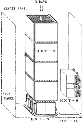
2.4 Schematic of the Hard X -ray Telescope onboard Y o h k o h... 50
2.5 The SoHO spacecraft and its suite of 12 instrum ents ... 52
2.6 Schematic of the halo orbit of the SoHO spacecraft at the LI La-grangian point...54
2.7 Schematic of the Extrem e-ultraviolet Imaging Telescope ... 55
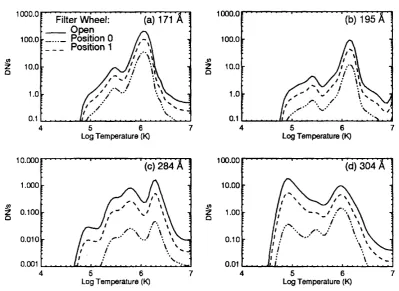
2.8 Temperature response of the Extrem e-ultraviolet Imaging Telescope fllte rs ... 58
2.9 Schematic of the optical layout of the LA SC O /C l coronagraph . . . . 60
2.10 Schematic of the optical layout of the L A SC 0/C 2 coronagraph . . . . 62
2.11 Schematic of the optical layout of the LA SC 0/C 3 coronagraph . . . . 63
2.12 Schematic of the Michelson Doppler Imager ...65
3.1 Example of the formation of post-eruption loops in active region 7999. 71
L IS T OF FIGURES 6
3.2 LASCO height-tim e plot of the coronal mass ejection on 30-Nov-96 . 72
3.3 Flare survey results; normalised flare duration versus the time differ
ence between CME launch and flaring...78
3.4 Flares survey results; normalised flare intensity versus the time dif
ference between CME launch and f l a r i n g ...78
3.5 Histogram of the product of normalised flare intensity and duration
for those flares occurring before the CME in the flare s u r v e y ... 80
3.6 Histogram of the product of normalised flare intensity and duration
for those flares occurring after the CME in the flare survey... 80
3.7 Flux evolution in active region 8 1 0 0 ...82
3.8 Flaring activity in active region 8100... 84
4.1 MDI photospheric flux distribution in active region 8100 at central
meridian on 2-Nov-1997 during the first rotation... 96
4.2 Evolution of the flux in active region 8100 at successive central merid
ian passages during five solar rotations... 97
4.3 MDI photospheric flux distribution in active region 8100 at central
meridian passage during rotations two to four...99
4.4 Evolution of the photospheric flux and soft X -ray loops for active
region 8100 during five solar rotations...101
4.5 Histogram illustrating the number of coronal mass ejections from ac
tive region 8 1 0 0 ... 106
4.6 Illustration of the rotation p h a s e s ... 106
4.7 Extrapolation of the coronal f i e l d ... 113
4.8 MDI photospheric flux distribution of the emergence of active region
8 1 0 0 120
4.9 Schematic of the emergence of a twisted emerging flux tu b e...121
5.1 LA SC 0/C 2 data revealing the absence of a coronal mass ejection
5.2 LA SC 0/C 3 data revealing the absence of a coronal mass ejection
associated to the X I.2 flare on 30-Sep-2000... 128
5.3 EIT 304 Â bandpass data showing the topology of plasma on 30-Sep-00 19:19 UT and 1-Oct-OO 01:19 U T ...130
5.4 Time series of EIT 195 Â bandpass images revealing the configuration of plasma at a tem perature of 1.5 x 10® K ... 131
5.5 Time series of SXT full resolution A112 filter data indicating the ex panding loop and soft X -ray plasmoid-like feature... 132
5.6 SXT A112 filter full resolution images before and after the start of the confined flare... 133
5.7 SXT A112 filter light curves of loop a and b...134
5.8 Temperature evolution of the flare l o o p ...135
5.9 Temperature evolution in the flare region...136
5.10 SXT A112 filter full resolution images prior to and after flare, overlaid with the contour of the emission from the Hard X -ray Telescope M2 channel... 137
5.11 Hard X -ray Telescope light curves of all four energy channels... 138
5.12 Hard X -ray Telescope flare footpoints in the HI channel ... 139
List o f Tables
1.1 Classification of active r e g io n s ... 27
1.2 Flare p h a s e s ... 32
2.1 List of filters mounted on the dual filter wheel of S X T ... 47
2.2 The scientific instruments onboard S o H O ... 56
2.3 Peak tem peratures of the Extrem e-ultraviolet Imaging Telescope fil ter bandpasses...57
2.4 Details of the coronagraphs on the Large Angle and Spectroscopic Coronagraph...64
3.1 Table of survey results... 75
4.1 Flux measurements in AR 8100 at central meridian passages during five solar rotations...98
4.2 Details of the coronal mass ejections originating in active region 8100 104 4.3 Observed and corrected coronal mass ejection number in active region 8 1 0 0 ...107
4.4 Helicity injection by differential rotation in active region 8100 . . . . I l l 4.5 Frequency of coronal mass ejections from active region 8100 and the expelled helicity... 117
This thesis seeks to understand further the role of solar flares and coronal mass
ejections in the evolution of the solar corona, and the relationship between the
two phenomena. The thesis starts with a description of the solar atmosphere and
the physics governing the magnetic flelds in this region. Active regions are then
discussed as they are the location of the flares studied in this thesis, and are related
to the coronal mass ejections selected. The magnetic flux which emerges into the
active regions is likely to be twisted and distorted. Such structure in the fleld can be
described by the param eter magnetic helicity, which is also introduced. A discussion
on coronal mass ejections and their relationship to flares and helicity concludes the
introduction section.
Various instruments have been used in order to obtain a complete analysis of
the chosen events. These instruments include both space-borne and ground based
instruments. There is a section to explain the workings of each instrum ent which in
clude the Yohkoh Soft X -ray Telescope and Hard X -ray Telescope, SoHO Extrem e-
ultraviolet Imaging Telescope, Large Angle and Spectroscopic Coronagraph and
Michelson Doppler Imager, the GOES X -ray flux monitor and two ground based
H a telescopes in Austria and Japan. The various d ata analysis techniques are also
briefly described.
The relationship between coronal mass ejections and flares has been debated
since the 1970s. This thesis investigates the effect of the ejections on the long-term
flare activity in certain active regions near solar minimum. It is found th at the
ejections significantly alter the magnetic environment in the flaring active regions
A B S T R A C T 10
to produce a situation where less energetic flares occur. It is also found th a t at the
start of a period of high CME activity in one particular active region, an imbalance
between the positive and negative line of sight magnetic flux forms. This may
also be related to a change of the magnetic environment resulting from a process
contributing to CME onset, or even possibly as a direct consequence of the CME
itself. The magnetic fleld component along the observers line of sight is measured
and so will be sensitive to changes in orientation of the field.
Coronal mass ejections are thought to be an im portant process in the solar corona
as they are the means by which plasma, and more importantly, magnetic fleld are
removed from one solar cycle to the next. Twisting and writhing of bundles of
magnetic fleld lines results in a quantity known as magnetic helicity which is a well
preserved quantity. Coronal mass ejections also therefore offer a natural method
to remove magnetic helicity and prevent an endless accumulation in the corona.
The source of helicity for a rotating active region which produces many coronal
mass ejections has been studied in this thesis. It has been found th a t the action
of differential rotation on the footpoints of the coronal flux tubes cannot provide
enough helicity to provide a source for the observed number of ejections. Instead
the source must be provided by the emergence of twisted and distorted flux from
below the photosphere.
The results in Chapter 3 are commensurate with previous work which suggests
th a t high intensity flares are likely to be accompanied by a coronal mass ejection.
Chapter 5 in this thesis details the study of a highly energetic flare th a t was expected
to be accompanied by a coronal mass ejection but was, in fact, confined to the lower
corona. It is found th at the flare is likely to be the result of an interaction between
emerging flux and pre-existing flux low in the corona. Reconnection occurs and
a fast expansion is observed in one of the loops. The work suggests th a t a fast
injection of twist into the expanding loop may have occurred, and th a t flares are a
In trod u ction
The Sun has posed a challenge to scientists for hundreds of years, and is the only
star th a t can be spatially resolved. The wealth of d ata collected by the many
space and ground based instruments over the years has revealed a variety of solar
phenomena on all observable spatial and temporal scales. Our understanding of the
physical processes taking place in the Sun has advanced substantially since the first
telescope observations were made by Galileo in the 17th century. However, many
questions on the phenomena th a t are observed remain unanswered. For example,
the heating mechanisms of the corona, the origin of the 11 year solar cycle and
the 22 year magnetic cycle, and the exact relationship, if any, between large scale
eruptions and small scale flares.
The Sun is a giant ball of plasma, considered on short time scales as being ap
proximately in hydrostatic equilibrium. It is held together under its own gravitation.
The first observations of the Sun were those made with the naked eye, and there
fore in white light. Sunspots were observed as early as 350 B.C. by Theophrastus
of Athens, a pupil of Aristotle, giving the indication th at the Sun was not perfect
and blemish free. Longterm observations of sunspots revealed the nature of surface
rotation and also the existence of a sunspot cycle. In fact, the Chinese have ob
servations of sunspots dating back over 2000 years. The invention of the telescope
C H A P T E R 1. IN TRO D U C TIO N 12
allowed more detailed observations of sunspots to be made, with seminal work car
ried out by Galileo Galilei in the 17th century. The most dram atic advances in solar
physics have been made with the ability to take observations above the E a rth ’s a t
mosphere. This allowed the Sun to be viewed in a totally new way using parts of
the electromagnetic spectrum normally attenuated by the E a rth ’s atmosphere. Most
significantly, observations could be made of plasma em itting at extrem e-ultraviolet
and X -ray wavelengths.
The solar interior consists of the core, radiation zone and convection zone and the
atmosphere consists of the photosphere, chromosphere, transition region and corona.
The approximation th a t the Sun is in hydrostatic equilibrium most obviously breaks
down when considering the solar wind. This is the constant outflow of plasma, from
the Sun into interplanetary space, which occurs as a consequence of the continual
expansion of the hot corona into the near vacuum of space. This chapter presents an
overview of the solar atmosphere and magnetic fields along with the theory governing
the behaviour of the system. The param eter magnetic helicity is introduced as it is
of param ount importance to the study of of magnetic fields in relation to eruptive
phenomena.
1.1
T he Solar A tm osphere
1.1.1
T h e P h otosp h ere
Viewing lower into the atmosphere of the Sun shows th a t the opacity (the ease
at which radiation can pass through the medium) increases. The point at which
the atmosphere appears to become completely opaque to radiation is known as the
photosphere, and is regarded as the imaginary surface of the Sun. It is an extremely
thin layer where the solar photons created in the core, become able to pass through
the solar atmosphere suffering only weak absorption. Below this region the opacity
The photosphere can be defined as the region from which the light escapes, a mere
100 km in thickness, centered on T = 5000 K and using an optical depth of unity. An
alternative definition is th at it is the region between 6600 K (base of photosphere)
and the tem perature minimum 4300 K, which is 500 km above the base of the
photosphere. It has an effective blackbody tem perature of 5800 K and the emission
peaks at visible and infra-red wavelengths. The photosphere is in continual motion
as a result of convection cells in the convection zone below which overshoot to
produce granulation cells with a thickness of around 100-200 km. The centre of
the cells appear bright in comparison to the boundary due to the hot plasma rising
from below (0.4 km s“ ^) which then moves horizontally (0.25 km s~^) to the cell
boundary where it sinks as cooler plasma. The diameter of the granulation cells
is typically 700-1500 km and they have a lifetime of around 8 minutes. A larger
scale velocity pattern known as supergranulation also exists. Supergranule cells are
typically 20000 - 54000 km across with a lifetime of 1-2 days. The convective flows
here are weaker than in the smaller scale granules and the m aterial rises in the centre
of the cells with a velocity of 0.1 km s ^ \ moves horizontally at around 0.3-.4 km
s~^ and sinks at the edge of the cell at 0.1-0.2 km s~^.
1.1.2
T he Chrom osphere
Moving up in the solar atmosphere, in both height and tem perature, leads into the
chromosphere. This region of the solar atmosphere extends from approximately
500 km to 2300 km above the base of the photosphere. Disc observations of the
chromosphere can be made using the light of H a (formed by the n = 3 to n = 2
Balmer transition, 6563 Â) and the Ca II H and K lines (3968 Â and 3934 Â). N on-
visible wavelengths are used to observe the hotter regions of the upper chromosphere,
such as ultra-violet (UV; 1000 Â - 3500 Â) and extreme ultra-violet (EUV; 100 Â -
C H APTE R 1. INTRO D U CTIO N 14
PHOTO SPHERE
CHROMOSPHERE TRANSI TION REGION
LOW CORONA
8600 28000 75000
LOW MIDDLE HIGH LOG T
TEMPERATURE MINIMUM REGION
2000 3000
0 1000 4000 5000 6000
HEIGHT (km)
The supergranulation boundaries are observed in the Ca II K line and observa
tions in H a near the limb reveal plasma jets known as spicules (Beckers 1972) in
the boundaries of the supergranules. H a observations on the disc reveal horizontal
features known as fibrils located at the supergranule junctions.
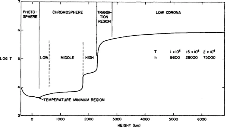
The tem perature increases in the atmosphere from the base of the chromosphere
and becomes extremely rapid in the interface between the chromosphere and the
corona, in a region known as the transition region. In the transition region the
tem perature rises from tens of thousands to over 1 million K. The tem perature
structure of the solar atmosphere is shown in Figure 1.1.
1.1.3
T he Corona
The tem perature rise continues into the solar atmosphere, to the region known as the
solar corona, where tem peratures of 2 million K are reached. The corona lies above
the chromosphere, and plasma with different tem peratures co-exist in this region.
The first indications th a t the solar corona was extremely hot and tenuous (10® cm"®)
came from the observations of emission lines from forbidden transitions (eg. Fe X
line at 6374 Â, Edlén 1942). These are transitions which proceed slowly. In a gas
of moderate density, collisions would destroy the excitations before a spectral line
can be emitted. However, in the hot tenuous plasma of the corona, these transitions
can be dominant. Observations of the corona cannot normally be made due to the
overwhelming photospheric emission (the coronal intensity is approximately one-
millionth of the photospheric intensity). However, white light observations can be
made at times of eclipse, or with the use of a coronagraph which produces an artificial
eclipse. Direct images can be taken in ultraviolet, extreme ultraviolet or X-rays as
the plasma emits thermally at the coronal tem peratures. The reasons for the high
tem perature of the coronal plasma are still disputed, but several mechanisms have
been proposed, and it may be th at different mechanisms are responsible for heating
C H APTE R 1. INTRO DU CTIO N 16
the first encompassing heating due to the dissipation of waves generated at the base
of the corona. The second group involves the dissipation of free magnetic energy
created by the shuffling of the fiux tube footpoints due to photospheric motions.
Recent work has indicated th at coronal heating models based on the stressing of the
coronal fields by footpoint motions, better fit the observational constraints than do
those models based on wave dissipation (Mandrini et al. 2000).
Soft X -ray images of the Sun were first taken using instrum ents flown on rock
ets, the typical angular resolution being 2 arcminutes. The first high resolution (few
arcsec) soft X -ray images of the corona were taken with the grazing incidence tele
scope onboard Sky lab (Vaiana et al. 1977). It was later realised th a t the observed
structure in the corona is dominated by the magnetic fields and can be roughly
divided into two regions; regions where the magnetic field is open and extends into
the interplanetary medium, and regions where the field is closed with both ends of
the flux tube intersecting the photosphere. In X -rays the closed field regions appear
as coronal loops in a range of sizes and topologies, associated to both the quiet Sun
and the concentrated magnetic fields above sunspots. The open field regions appear
dark due to the outflow of plasma to form coronal holes and the fast solar wind.
Open field lines are defined to be those which extend outward beyond the height at
which the velocity of the solar wind becomes super-sonic.
1.1.4
Em ission P rocesses
To observe the corona against the overwhelming emission of the photosphere, very
long wavelengths (eg. radio) or very short wavelengths (eg. X-ray) must be used.
The lower tem perature of the photosphere means th a t it appears dark in X-rays, and
at radio wavelengths, the height at which the optical depth reaches unity occurs high
in the atmosphere, allowing observations in the corona. The coronal gas radiates
efflciently and is dominated by isolated spectral lines from trace elements, on top of
and helium are almost completely ionised and do not contribute significantly to the
emission.
The hot (T > 2 X 10^) plasma in the solar atmosphere has a low density
(rig < 10^^) and it is assumed th a t the plasm a is in a steady state. That is, th at
the collisional excitation of an atomic species (X) from level i to j is balanced by
the non-collisional process of spontaneous decay. An ion in an excited state can
spontaneously emit radiation when the electron falls to a lower energy state, and is
given by:
x + ’^ + huij (1.1)
where an atom X of charge state + m in a quantum state j is denoted by X^ '^.
This decay process emits a photon, and is known as bound-bound emission. The
energy of the photon is equal to the energy difference between the quantum states
i and j of the ion (Eq. 1.2).
AEi j {erg) = hi^ij (1.2)
In the coronal equilibrium model it is assumed th a t the upper state, j, is popu
lated mainly by collisional excitation by free electrons and th a t the de-population
occurs by radiative decay. This process produces spectral lines, the intensity of
which, at a wavelength Xij from a column of plasma with volume V and cross-
sectional area A, per unit solid angle, is given by Eq. 1.3.
nki) = ^ f v P ( K j ) d V
(1.3)The units of Eq. 1.3 are erg cm“ ^ s“ ^ sr~E P(A*j) is the emissivity (power per
unit volume) of the line, given by
C H APTE R 1. IN TRO D U CTIO N 18
where Nj{X^'^) (cm"^) is the number density of ions in quantum state
j and Aj^i (s“ ^) is the Einstein spontaneous emission coefficient (a measure of the
number of transitions from state j to state i occurring per second).
Along with bound-bound emission, the coronal spectrum also consists of bound-
free and free-free emission. These processes become especially im portant at coronal
tem peratures due to the large number of free electrons present in the coronal plasma.
The low mass of the electron means th at they can be easily accelerated, and they also
radiate efficiently. Scattering of the electrons from ions results in Bremsstrahlung
radiation, or free-free emission. Capture of the electrons by ions produces free-bound
emission. Both of these processes produce a broad continuum of radiation.
1.2
M agnetic Fields
The realisation th at the Sun is magnetic star came with the discovery of the Zeeman
effect in sunspots by Hale (1908). All forms of solar activity are now thought to be
related to the magnetic fields threading the Sun which are able to store energy th at
can then be released to power energetic phenomena when the field deviates from
the potential configuration. The structure in the corona is dictated by the magnetic
field due to the large energy density of the field compared to th at of the plasma.
There is a continual supply of magnetic fiux to the corona via the rise and emergence
of flux created at the base of the convection zone.
1.2.1 G eneration o f M agnetic F lu x
It has been known since the time of the first sunspot observations th a t the photo
sphere rotates differentially and not as a solid body. Observations of the motion of
the sunspots across the disc revealed th at the rotation velocity reduces at higher
latitudes. The differential nature of the rotation continues down through the con
vection zone to its base. Here, in the deeper layers of the Sun, the rotation becomes
known as the tachocline, and is thought to be the location of the solar dynamo (for
two good reviews see Deluca & Gilman 1991; Fisher et al. 2000). The dynamo pro
vides the continual regeneration of magnetic field from the motions of the electrically
conducting plasma which is embedded in a ’seed’ background magnetic field. It is
a way of converting the plasma kinetic energy into magnetic energy. The plasma
and the magnetic field are frozen together as a result of the high electrical conduc
tivity (see section 1.2.2), so the plasma is forced to move through the background
magnetic field due to the convective motions. When a conductor (the plasma) is
moved through a magnetic field it experiences a force and responds by moving. This
motion is itself a current and induces an additional magnetic field.
The solar dynamo produces a poloidal magnetic field, the lines of which are drawn
out due to the faster rotation velocities at lower latitudes and wrapped around the
Sun becoming parallel to the equator (Cowling 1953; Babcock 1961). Regions of
strong magnetic field form flux tubes which are able to rise through the convection
zone by magnetic buoyancy. Consider the internal and external forces on a fiux tube
in pressure equilibrium embedded in an unmagnetised plasma; the external pressure
{Pext.gas) ÎS due to gas pressure only and the internal pressure is due to the internal
gas pressure (Pint.gas) and magnetic pressure ( ^ ) where B is the magnetic field.
The pressure balance is then given by,
Pext.gas ~ Pint.gas T (1-5)
We know from the ideal gas law (Eq. 1.6) th a t gas pressure is proportional to
density and tem perature. This means that, assuming equal internal and external
tem perature, the density inside the fiux tube is less th an th a t of the surrounding
plasma and the tube will be buoyant and can rise to the photosphere.
P = ~ (1.6)
C H APTE R 1. INTRO D U CTIO N 20
T is the tem perature and V is the volume.
The result is the rise of an Q shaped loop through the convection zone if the
footpoints of the flux tube remain anchored. The term inal velocity of a flux tube, v,
is given in Eq. 1.7 as found by Parker (1975). The tube rises at a rate determined
by the balance of buoyancy and aerodynamic drag.
" =
(âp)
where R is the radius of the flux tube, is the drag coefficient, Hp is the
pressure scale height and va is the Alfven velocity in the flux tube (Eq. 1.8. The
pressure scale height is the distance over which the pressure falls by 1/e.
/ ^2 \ 1/2
The journey of the flux tube up through the convection zone is not straight
forward, and certain conditions must be met for the tube to remain coherent, ie.
intact, during its rise. Schiissler (1979) and Longcope et al. (1996) showed th a t at
the beginning of the rise phase a buoyant flux tube in tem perature equilibrium with
its surroundings will develope an umbrella shaped cross section, where the side lobes
rotate in opposite directions and detach themselves from the tube. The detached
sections experience a downward force which cancels the effects of buoyancy and the
flux tube ceases to rise, instead the tube experiences a horizontal motion. Emonet
& Moreno-Insertis (1998) showed th at for a flux tube to remain coherent during its
rise to the photosphere, and not be ripped apart by the vortices trailing the tube, a
certain amount of twist must be present so th at the magnetic tension prohibits the
formation of the vortex rolls. The amount of twist needed is given by a pitch angle,
of
1 R
^ « sin (1.9)
l i p
the location of the maximum transverse magnetic field, Emonet & Moreno-Insertis
(1998) find th a t a pitch angle of around 10^ is needed for the fiux tube to w ithstand
the destructive forces of the vortices.
1.2.2
E quations G overning th e M agn etic Field and Solar
P lasm a
The branch of physics describing the interaction of the magnetic field and an elec
trically conducting plasma is known as magnetohydrodynamics (MHD), MHD can
be used for sub-relativistic velocities, large scale phenomena where the length scales
are greater than the Debye length, collisional plasma or strongly magnetised plasma
and is therefore good for the solar corona. The Debye length gives an indication of
the distance over which the electrostatic field of a charge is shielded as a result of the
collective behaviour of a plasma. The electrostatic potential falls off exponentially
over a distance called the Debye length given by Eq. 1.10.
S
where k is Boltzmann’s constant, Tg is the electron tem perature, C[0 is the di
electric constant, Uq is the equilibrium density of the plasma with Tg and Çg is the
charge of electron. A typical value in the corona is around 1.7 cm (T = 3 x 10® K
and Tig = 5 X 10^) (Keenan et al. 1996).
To investigate how the magnetic field changes with time Ampere’s law (Eq. 1.12),
O hm ’s Law (Eq. 1.11) and Faraday’s (Eq. 1.13) law can be combined. When the
plasma velocities are much less than the speed of light, the displacement current
(second term in Eq. 1.12) can be neglected and Eq. 1.12 becomes V x B = /ij.
Using also the divergence free nature of the magnetic field, the resulting equation
(1.14) is known as the Induction equation where 77 = ^ is the Ohmic magnetic
diffusivity. In the following equations j is the current density, B is the magnetic
C H A P T E R 1. IN TRO D U CTIO N 22
field, /i is the magnetic permeability in a vacuum (47t x \ 0 ~ ^ a is the electrical
conductivity, V is plasma velocity and t is time.
J
=a{ E + V
Xê )
(1.11)V x B = ^ij + ~ (1.12)
V x Ê = ~ (1.13)
o D
— = V X ( f X B) + jjV^B (1.14)
The first term on the right hand side (RHS) of Eq. 1.14 represents the changes
in the magnetic field due to advective motions of the field with the plasma and the
second term represents the diffusion of the magnetic field through the plasma. The
ratio of the advective to the diffusive time scales gives the dimensionless param eter
known as the magnetic Reynolds number (Rm^ Eq. 1.15) where L and v are typical
length and velocity scales.
Rm = — (1.15)
ri
When Rm Z$> 1 the first term on the RHS of the Induction equation dominates
and the changes in the magnetic field can be taken to be due to the fluid motions.
When Rm 1 the second term on the RHS dominates and the changes in the
magnetic field are dominated by diffusion. In this situation the magnetic field lines
may slip across the plasma. The magnetic Reynolds number is proportional to the
length scale, the velocity and the electrical conductivity. In the situation where flows
occur at low values, the main factors determining the magnetic Reynolds number are
the length scales and the electrical conductivity. In the solar corona Rm = 10^ — 10^^
indicating th at diffusion is usually negligible and the induction equation reduces to
^ = V X ( y X B) (1.16)
As a consequence of this limit, the magnetic field lines are restricted to move
with the perfectly conducting plasma (Alfven 1942), this has become known as the
magnetic field lines being frozen into the plasma.
Many solar phenomena are observed to remain essentially static for long periods
of time and a m agnetostatic equilibrium solution to the MHD equations can be as
sumed. In magnetohydrostatics the equation of motion reduces to the force balance
equation (Eq. 1.17) as fiows are neglected.
0 = - T 7 P - ^ j x B + pg (1.17)
On the RHS, the first term is the pressure gradient, the second term is the Lorentz
force and the third term is due to gravity. From Ampere’s law (Eq. 1.12), the current
density can be substituted into the Lorentz force to obtain Eq. 1.18 where it can be
seen th a t the Lorentz force can be decomposed into a scalar magnetic pressure (first
term on RHS) and a magnetic tension force (second term on RHS).
The plasma /3 is defined as the ratio of the gas pressure to the magnetic pres
sure p = When the plasma (3 is large (z> 1) the plasma motions can shape
the magnetic field. However, when the plasma /? is low (<K 1) the Lorentz term
dominates in Eq. 1.17 and the energy density of the magnetic field is greater than
th at of the plasma. Such conditions exist above sunspots and active regions. In this
case the Lorentz force vanishes and the field is force-free to a good approximation.
The force-free condition (Eq. 1.19) can be used in the corona where the plasma j3
is much less than unity, b ut cannot be used in the convection zone and photosphere
CH A P T E R L INTRO D U CTIO N 24
j x B = 0 (1.19)
If the force-free magnetic field is not potential (the lowest energy state), the
general solution to the force-free equation (Eq. 1.19) is th a t the currents run parallel
to the magnetic field and V x B = a B , where a is a scalar function of position, a
is useful as it allows the determination of the amount of twist in the magnetic field
and therefore free energy.
1.2.3
M agnetic R econn ection
The solar atmosphere is normally assumed to be be a perfect conductor but un
der some situations this condition breaks down and diffusion ceases to be negligible
in Eq. 1.14. In these regions, known as diffusion regions, the frozen in theorem
breaks down due to the non-negligible diffusion, and the magnetic field lines are
able to change their connectivities through a process known as magnetic reconnec
tion (Dungey 1953; Sweet 1958a,b; Parker 1957). The simplest scenario is th at
of oppositely directed field lines separated by a thin current carrying layer (sheet)
which arises due to the change in field direction. The presence of a current on small
spatial scales, along with the locally enhanced resistivity means, th a t the diffusion
term in the induction equation cannot be neglected. The magnetic field lines are
then able to diffuse through the plasma. For steady reconnection the configuration
is such th a t oppositely directed magnetic fields are brought toward each other into
the diffusion region where they reconnect and are ejected. Figure 1.2 illustrates a
simple 2-D reconnection scenario of a X-type neutral point. Configurations such as
these are unstable, if the field lines are free to move (Dungey 1953) perturbations to
the field can trigger reconnection. The outflowing plasma can have velocities of the
order of the Alfven velocity, which is around 1000km s~^ in the corona. Topologies
where reconnection can occur include null points (regions of no magnetic field) in
c *
A*
Inflow region
B*
D*
Outfow region
C
D
Figure 1.2: Schematic of steady X -typ e reconnection. Field lines AB and CD are carried into the diffusion region where they reconnect to form A*C* and B*D*.
photosphere), or in the absence of these, reconnection can occur in quasi-separatrix
layers (regions where a large gradient in the magnetic connectivity occur). Recon
nection is of fundamental importance in the evolution of the coronal magnetic fields.
Observations show that these fields become twisted as a result of photospheric mo
tions (Parker 1987), and this results in energy being stored in the fields as they
become non-potential. Reconnection is a method by which the energy stored in
the magnetic field can be released and results in heating of the plasma. It is also
a very im portant process in the study of coronal mass ejections as it allows the
detachment of magnetic volumes from the photosphere which can subsequently be
ejected. It also allows energy to be extracted from the field which is though to drive
C H APTE R 1. IN TRO D U CTIO N 26
1.2.4
M agnetic H elicity
The complexity of the coronal magnetic field, such as twist and writhe, is best
described by the param eter known as the magnetic helicity (hereafter referred to as
helicity). In the solar corona, the magnetic field pervades the space and it is useful
to use the concept of a magnetic flux tube. A magnetic field line is everywhere
parallel to the magnetic field B (B x dl = 0). Following from this, a flux tube is
a collection of field lines which intersect a simple closed curve. The strength of the
flux tube is given by the flux crossing a cross-section of the tube, and is constant
along it ’s length. The twist in the magnetic field is the rotation of the field lines
about the axis of the tube, and the writhe is the rotation of the axis of the tube
in space. The helicity of a field B within a volume V is defined by (Moreau 1961;
Moffatt 1969, 1978, 1981):
H = j
A . B d V , (1.20)where  is the vector potential which satisfies,
B = V x  . (1.21)
Eq. 1.20 is physically meaningful only when the magnetic field is fully contained
inside V (i.e. at any point of the surface S surrounding V, the normal component
Bn = B . n vanishes); this is so because the vector potential is defined through a
gauge transformation (A' = A-h V $ ), and H is gauge-invariant only when Bn = 0.
Berger & Field (1984) have shown th at for cases where ^ 0 one can define
a relative magnetic helicity {Hr) by subtracting the helicity of a reference field Bq,
having the same distribution of Bn on S. The relative magnetic helicity is given by,
Hr = A . B d V - Ao.BodV (1.22)
Berger & Field (1984) and Finn & Antonsen (1985) have shown th a t Hr is
gauge-invariant, and th a t Hr does not depend on the common extension of B and
Helicity is a conserved quantity under conditions of high magnetic Reynolds
number in both ideal and resistive MHD conditions, on timescales short compared
to the global diffusion timescale. Berger & Field (1984) give a diffusion time of 10^
years.
1.3
A ctive R egions
1.3.1 D efinition
Measurements of the photospheric magnetic field revealed the existence of regions
of intense field strength (3-4000 Gauss), in a relatively field free background. These
strong field regions were observed to be spatially coincident with sunspots are inter
preted as being the intersection of flux tubes, created at the base of the convection
zone and buoyed up into the corona, with the photosphere. X -ray and Extreme
Ultra-violet observations showed th a t the flux tubes manifest themselves in the so
lar atmosphere as a complex system of loops. Active regions (ARs) comprise the
sunspots and the extension of the flux tubes into the atmosphere. It is useful to
classify the degree of magnetic complexity in an active region, which changes as
the region evolves and also leads to different levels of activity. They are classed by
the complexity of the magnetic field as observed at the photosphere and Table 1.1
details the NO A A classification scheme.
Table 1.1: Classification of active regions by their m agnetic complexity, courtesy of NO A A.
Class Description
a All magnetic measurements are of the same polarity
j3 A bipolar group
7 A group in which the polarities are intermingled
Ô A group containing spots of opposite polarity within 2°
C H A P T E R 1. INTRO D U C TIO N 28
1.3.2
T opology o f th e M agnetic Field
Active regions are the result of magnetic flux which has traveled from the tachocline
up through the photosphere to produce loops in the corona. As the flux tubes
created at the base of the convection zone rise, their shape resembles th a t of the
letter 0 . The loops rise and expand, and rotate due to the action of the Coriolis
force. The motions are clockwise in the northern hemisphere and anti-clockwise in
the southern hemisphere. This is known as Joy’s Law and results in the leading spot
of the bipolar sunspot pair being located closer to the equator. This action results
in the creation of writhe in the tube and causes the tube to be inclined so th at the
leading spot is further from the magnetic neutral line than the following spot, ie.
there is an eastward tilt.
W hilst the flux tubes are traveling through the convection zone they may be
affected by turbulent motions which are thought to have a helical nature. There
is a hemispheric dependence in these helical motions, again due to the action of
the Coriolis force on expanding up-flowing, and contracting down-flowing turbulent
motions. The helical turbulence imparts writhe of the same sense into the flux tubes
which then develop twist of the opposite sense to conserve helicity. Longcope et al.
(1998) discuss the effects of these helical turbulent motions on an initially horizontal
flux tube rising through the convection zone and find th a t a significant amount of
twist can be im parted into the flux tubes as compared to twist contained in AR
fields inferred from observations.
The result of Joy’s Law acting on the flux tubes means th a t the footpoints
of the tube at the photosphere will lie at different latitudes and so will rotate at
different velocities, with the lower latitude footpoint rotating faster. Eq. 1.23 gives
the classic formula for differential rotation where (p is solar latitude and u is the
rotation rate. Komm et al. (1993) used K itt Peak magnetograms from 1975-1991 to
Lü{(f)) = a T bsin^ ( j ) c s i n ÿ (1.23)
Over long timescales, differential rotation can inject helicity into the coronal
flux tubes. Active regions in the northern (southern) hemisphere are injected with
negative (positive) helicity (Devore 2000). Longlived active regions can have their
helicity content increased or reduced by the action of differential rotation, depending
on the initial helicity content and inclination to the equator. Démoulin et al. (2001a)
showed th a t the helicity generated in a coronal flux tube by differential rotation is
composed of two components; twist and writhe. The motion of the footpoints
relative to each other im parts writhe into the tube, but differential rotation will
rotate each footpoint and inject twist. The computations of Démoulin et al. (2001a)
show th a t for shear regions close to the neutral line of a bipolar AR the effects of
twist and writhe add up. For more extended shear regions the twist and writhe are
of opposite sign and are in competition, and this situation is relevant to the shear
profile of differential rotation on ARs.
Section 1.2.1 discussed theoretical work th a t indicated emerging flux should al
ready contain twist and writhe. This has been supported by observations which have
shown the presence of currents associated to the emerging flux, therefore indicating
twist in the newly emerging field (Leka et al. 1996). The helicity content of emerged
flux can then be added to or reduced by the effect of differential rotation at the
footpoints of the coronal field. Therefore, it can be expected th at newly emerging
flux will contain helicity, carry currents and contain free magnetic energy.
1.3.3
A ctive R egion Flares
Magnetic reconnection is the process by which the free energy stored in the AR
fields can be released. One common product is a solar flare where more than 1 0^^
ergs of energy is released over a few minutes producing emission throughout the
C H A P T E R 1. IN TRO D U CTIO N 30
region is complex and current carrying flux is still emerging. The mechanism to
describe flares needs to involve fast reconnection to reproduce the short observed
timescales for energy release and such a mechanism was first described by Petschek
(1964). In this model, two pairs of slow-mode magnetoacoustic switch-olf shocks
extend from the diffusion region and magnetic flux is carried through them. The
magnetic field vector rotates toward the normal producing a decrease in the strength
of the magnetic field which converts the magnetic energy into heat and kinetic
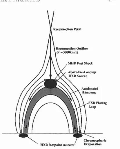
energy of accelerated particles. A schematic of a simple loop solar flare is shown in
Figure 1.3 (Masuda 1994), illustrating the observational aspects. In this scenario a
hard X -ray source is produced at the loop top as the outflow from the reconnection
region impinges on the dense material in the loop. The flaring loop becomes bright
in soft X-rays as the accelerated particles collide with the chromosphere and produce
ablation of the chromospheric material.
Several models have been proposed to account for the observational aspects of
solar flares which exhibit many different topologies, durations, size scales and spec
tral evolution. It has been proposed th a t generally flares fall into two categories,
compact flares and long duration events (LDEs) (Pallavicini et al. 1977). Compact
flares normally involve simple loops, small size scales and have an impulsive nature.
One model for these flares is the emerging flux model proposed by Heyvaerts et al.
(1977). Conversely, LDEs are thought to involve large magnetic structures and have
a prolonged gradual phase. LDEs are sometimes called eruptive flares as they are
thought to be associated to the closing down of magnetic field opened during an
eruption. This idea arises from observations of flare ribbons which move apart with
time and also the increasing height of the flare-loops as reconnection progresses
higher in the atmosphere. These flares are often observed after prominence erup
tions as in the CSHKP model (Carmichael 1964; Sturrock 1966; Hirayama 1974;
Kopp & Pneuman 1976). In this model a filament eruption, triggered by a global
instability, is the means by which the underlying magnetic field is stretched open
Reconnection F^nt
fUconnection Outflow <v--3<KKfcm/s)
Fa$t Shodc
Above-tJie- Looptop HXR Sourco
HXR footpoint sources
C H A P T E R 1. INTRO D U CTIO N 32
erupted filament to produce the LDE as successively higher magnetic field lines
reconnect. However, the idea th a t only long duration flares occur with CMEs is
misleading. Harrison (1 9 9 5 ) shows th a t even though long duration flares are com
monly CME associated, the flares occurring at CME time can be of any duration.
In general, the flare process can be split into four phases as is shown in Table 1.2.
Table 1.2: Flare phases and their manifestations in the solar corona.
Phase Manifestation
Precursor Transient soft X -ray and microwave enhancements, and
line broadening are occasionally observed up to 10 min
utes before the flare
Impulsive Phase Most evident in hard X -ray and radio, emission also in
optical, UV, XUV, 7-ray and microwave.
Gradual Phase Slow increase in soft X -ray emission, lasting several min
utes to lO’s of minutes
Decay Decay in soft X -ray emission
1.4
Coronal M ass Ejections
1.4.1 D efinition
Coronal mass ejections are transients of m aterial moving out through the corona (see
Figure 1.4). They involve the expulsion of plasma from the solar atmosphere, over
a large spatial extent, driven out against the gravitational pull of the Sun. The first
observations of CMEs were made in the 1970s by space-borne coronagraphs; instru
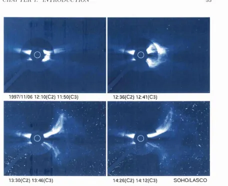
1997/11/06 12:10(C2) 11:50(C3) 12:36(C2) 12:41(C3)
13;30(C2) 13:46(C3) 14:26(C2) 14:12(C3) SOHO/LASCO
Figure 1.4: Composite LASCO C2 and C3 images of a coronal mass ejection on 6-N ov-1997. Courtesy of SOHO/LASCO consortium.
the overwhelming photospheric emission. Such instruments offer substantial advan
tages over ground based coronagraphs which suffer from scattered skylight, limit
ing observations to those close to the solar disc. Space-borne coronagraphs suffer
only from stray light generated within the instrument itself, and LASCO therefore
offers an increased field of view and a greater sensitivity than ground based instru
ments (eg. MacQueen et al. 1974; Hildner et al. 1975; Gosling et al. 1976). They
exhibit a range of morphologies from the classical 3-part structure of an expanding
loop followed by depleted region containing bright filament material, to amorphous
CH A P T E R 1. INTRO D U CTIO N 34
had a median size of 50 degrees and a median velocity of 360 kms“ ^ (St.Cyr et al.
2000) but can be as fast as 2000 kms~b They can have a mass in the order of 10^^
g and cause interplanetary effects due to their mass and the magnetic flux which
threads them. They are observed by the Thomson scattering of photospheric light
off the coronal electrons, the intensity of which is proportional to the electron den
sity. From the point of view of the observer, the greatest contribution comes from
density structures in the plane of the sky, hence CMEs are more easily observed
when they originate on the limb.
1.4.2
Coronal M ass E jections and th eir R elation sh ip to A c
tive R egion Flares - H istorical R eview
Since the discovery of CMEs in the 1970s much effort has been made to understand
the drivers and the on-disc counterparts for the ejection. An association to flaring
was quickly made as energetic events on the sun were sought to understand the
launch process of the CME (Dryer 1982). Previous work has been based on the
assumption th at the CME has an ’associated’ flare, ie. th a t in some way they are
causally connected. However, this ’associated’ flare is one of many th a t may occur
in the region which eventually produces a CME, and is the one which happens to oc
cur closest temporally to the launch of the CME. A common conclusion in previous
work has been th a t the probability of a CME occurring with a flare increases with
the intensity of the accompanying X -ray flare (Burkepile et al. 1994; Munro et al.
1979, for example). The relationship between flare duration and CME occurrence
has also been studied and has indicated th a t CMEs occur preferentially with long
duration events (Sheeley et al. 1983). Webb & Hundhausen (1987) found a good
correlation between long duration events and the occurrence of a CME, as did Har
rison (1995). The physical interpretation of the process connecting LDEs and CMEs
has been described by the CSHKP model (see Figure 1.5). However, no model has
although it should be noted th at the m ajority of high intensity flares tend to be long
duration events which are then consistent with the CSHKP model. For impulsive
high intensity flares, Kahler et al. (1989) found from a study of impulsive events
during 1979-1982, th at 2 2% were associated to CMEs. Two thirds of the X -ray
events in this study, which were GOES class XI or greater, were accompanied by a
CME.
Further research indicated th at the flares which occur close in time to the CME
onset have a rise phase which begins after the CME has begun to lift off. Harrison
(1986) used data from SMM and observed a weak soft X -ray burst (the precursor)
which preceded the flare by several 10s of minutes and during which the CME
appeared to be launched. N itta & Akiyama (1999) also found the CME to precede the
flare, however observations of CME onset after the flare are not unknown (Hudson
& Webb 1997). Harrison (1995) used a larger dataset (30 events) and found th at
the flare and CME may occur anytime within a few tens of minutes of each other.
Clearly, any temporal relation between the flare and an associated CME is still open
to debate. For this question to be resolved a CME launch time using lower coronal
signatures needs to be determined. The current method of finding CME launch
times uses the position of the CME front as observed in coronagraph data. The
CME motion is then extrapolated back in time without the knowledge of the initial
height of the pre-CM E structure in the corona and this introduces large errors in
the estim ated onset time.
Even before CMEs were discovered in coronagraph d ata it was thought th a t flares
could expel material by the production of a hydrodynamic blast (Parker 1961). How
ever, the idea th at the flare is the cause of the CME is now outdated due to the
observations of asymmetry in the size and location of flares and CMEs (Harrison
1986), but the strongest evidence comes from the indications th at the CME is ini
tiated before the flare. Zhang et al. (2001) showed th a t although the CME may be
initiated before the flare, there is an impulsive acceleration of the CME at the time
C H APTE R 1. INTRO D UCTION 36
a) P r e - f l a r e
c) Late P h a s e
rising
prominence
IPS
loookm
' y
-b) Maximum Phase
b’) Maximum; side view
2 sh o c k
rising
m a s s
flow
co m p re ssio n
h e a t
flow
j l oookm
lO^K two ribbon f l a r e
active region chromosphere
acceleration of an erupting filament during the rise phase of the fiare. This indicates
th at there may be some relation between the fiare and the CME even if they are not
cause and effect. Earlier work by Kahler et al. (1988) studied the development of
filament eruptions during the impulsive phase of the solar flares. The authors found
th a t in only two of the four events studied, impulsive acceleration of the filament
was observed.
Bruzek (1952) proposed th at flares were the source of fast and slow mode waves,
and th a t the slow mode waves may activate filaments and result in an eruption.
However, Rust (1997) found th at the source of the slow mode waves may be the
activated filaments themselves and if the disturbance follows a fiare it is only because
a filament activation preceded it. In addition, Khan & Hudson (2000) have discussed
flares as the cause of CMEs, with observations of three CME events which occur after
major flares. The observations suggest th a t shock waves from the flares destabilises
large transequatorial loops resulting in a CME. The shock waves are launched from
an active region which is situated at one end of the then destabilised structure. This
work suggests th a t in some cases the fiare may be vital to the launch of an ejection.
However, observations of a single fiare th at could trigger a CME are uncommon and
the emphasis remains in there being no cause and effect between the fiare and CME.
Previous work seems to suggest th at they are all p art of the coronal response to a
destabilisation of the field on a local and global scale, as was suggested by Harrison
(1996).
1.4.3
CM E Launch M echanism s
Models describing the launch of CMEs must account for the large velocities th a t
can be attained and the opening, or partial opening, of the magnetic field. CMEs
involve the expulsion of around 1 0^® g of solar plasma with energies of around 1 0^^
ergs and it is generally accepted th at the only source of energy large enough to
C H A P T E R 1. INTRO D U CTIO N 38
fields (Forbes 2000). A restriction on CME models is th a t they must not violate the
energy requirements set by the Aly-Sturrock conjecture (Aly 1984, 1991; Sturrock
1991). This conjecture results from computations of force-free fields which have
shown th a t the closed field configuration contains less energy than the open field
situation. Therefore, the open field configuration is the highest energy state and so
can never be reached by a process which requires the release of stored energy from
the field. In this case, closed magnetic field cannot eruptively be fully opened to
infinity.
Most CME models are based on the ideal MHD situation where the configuration
is th a t of a twisted flux rope and/or a sheared arcade and the field in the corona is
assumed to be force-free. Twisted flux ropes are found in active regions as well as
in quiet Sun regions, and can support relatively cool and dense plasma in the dips of
the magnetic field to form prominences. Quiescent filaments are large scale features
which form as active regions grow old and decay, and represent the later stages of
an ARs life. Helical structure has been observed in erupting filaments, and flux
ropes th a t are sufficiently twisted may erupt after becoming unstable to the kink
instability (Rust & Kumar 1996). The kink instability is an ideal MHD instability
occurring when the twist of the field lines around the flux tube exceeds a critical
value, resulting in an eruption. Priest & Hood (1979) gives the critical value under
force-free conditions to be 0 = 2.57T, where (j) is the angle made by the twisted field
line in going from one end of the tube to the other.
In the ideal MHD situation, flares may occur as a by-product of the instability.
When field lines are stretched open they are at a high energy state and reconnection
will occur in the current sheet closing the field lines back down to a lower energy
level. Lin et al. (1998) use a combination of ideal and non-ideal MHD to describe
the CME launch. They found th at the loss of ideal MHD in a curved flux rope can
lead to the formation of a current sheet and if rapid reconnection occurs, the flux
rope will be expelled from the Sun. The Aly-Sturrock constraint severely restricts