Nondestructive Evaluation Of Corrosion Damage In Reinforced Concrete Aged Slab Specimen

(1)

University of South Carolina

Scholar Commons

Theses and Dissertations

2018

Impact Of Critical Path Method (CPM) Of

Scheduling On On-Time Completion Of

Transportation Projects

Fahim Ahmed

University of South Carolina

Follow this and additional works at:https://scholarcommons.sc.edu/etd Part of theCivil Engineering Commons

This Open Access Thesis is brought to you by Scholar Commons. It has been accepted for inclusion in Theses and Dissertations by an authorized administrator of Scholar Commons. For more information, please [email protected].

Recommended Citation

(2)

I

MPACT OF

C

RITICAL

P

ATH

M

ETHOD

(CPM)

OF

S

CHEDULING ON

O

N

-T

IME

C

OMPLETION OF

T

RANSPORTATION

P

ROJECTS

by

Fahim Ahmed

Bachelor of Science

Bangladesh University of Engineering and Technology, 2014

Submitted in Partial Fulfillment of the Requirements

For the Degree of Master of Science in

Civil Engineering

College of Engineering and Computing

University of South Carolina

2018

Accepted by:

Nathan N. Huynh, Director of Thesis

Robert L. Mullen, Reader

Charles E. Pierce, Reader

(3)

(4)

DEDICATION

I dedicate this work to my parents, Sk Shafi Ahmed and Shirin Akter, and to my

beloved wife, Mishma. I thank them for believing in me, supporting through difficult times

(5)

ACKNOWLEDGEMENTS

I would like to express my sincere gratitude to my advisor, Dr. Nathan Huynh, for

his thoughtful guidance, patient, and support in completion of the thesis.

I am very thankful for the support, encouragement, and critiques of my thesis

committee members, Dr. Robert Mullen and Dr. Charles Pierce. I would also like to express

my appreciation to my lab mates and colleagues in my graduate school for all the help and

to make my journey more colorful and

Finally, I would like to thank the South Carolina Department of Transportation

(6)

ABSTRACT

This study addresses the effectiveness of Critical Path Method (CPM) scheduling

on project delivery. Specifically, the on-time completion of projects with and without a

CPM schedule is explored. The paper uses data from 2,097 South Carolina transportation

projects let after February 2008 and substantially completed by August 2015. The delay

analysis uses the original contract completion date as well as the completion date adjusted

by change orders. Chi-Squared tests are used to examine the relationship between CPM

scheduled projects and delayed projects, and t-tests are used to compare the mean delay (in

days) between CPM scheduled and unscheduled projects. The results of these tests indicate

that both the fraction of delayed projects and the mean delay (in days) are larger in projects

with CPM schedules. Several conjectures that explain these unexpected results are given.

A nationwide survey was conducted to find out the viewpoint on CPM schedules of state

Departments of Transportation(DOTs), resident construction engineers and contractors.

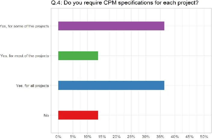
The survey revealed that most state DOTs use CPM along with Gantt chart for scheduling

and perceived complexity and risk are used to select projects for CPM schedules. Resident

construction engineers indicated that delay before the start of work on the field do not

impact the overall duration of the project. The contractors acknowledge the importance of

CPM schedules but they sometimes fail to make most out of CPM schedules. The issues

regarding selection criteria, enforcing and skilled person for CPM schedules are addressed

(7)

LIST OF TABLES

Table 2.1 Focus groups for standard specifications for construction of DOTs ... 14

Table 3.1 Topic focused on the survey for DOT headquarter personnel, Resident Construction Engineer and Contractors ... 24

Table 3.2: Lists of DOTs for phone interviews ... 26

Table 3.3 Raw project data description in SiteManager provided by SCDOT ... 27

Table 3.4 Description of different types of projects in the SiteManager database ... 29

Table 3.5 Database development and variables calculated ... 31

Table 4.1: Distribution of SiteManager Projects, SST Projects and SSPRIM Projects by Project Types ... 36

Table 4.2 Distribution of Projects by Project SCDOT districts ... 37

Table 4.3 Distribution of Projects by Project Size Groups ... 37

Table 4.4 Distribution of Projects by Project Duration Groups ... 37

Table 4.5 Impact of Using a Critical Path Method (CPM) Schedule on Project Delays by Project Type ... 38

Table 4.6 Impact of Using a Critical Path Method (CPM) Schedule on Project Delays by Project Size ... 40

Table 4.7 Impact of Using a Critical Path Method (CPM) Schedule on Project Delays by Project Duration groups ... 41

Table 4.8 Chi-Squared Test Results for Project Types, SCDOT Districts and Project Size Groups ... 43

(10)

Table 4.10 t-test Results for SCDOT Districts (Considering Original and Adjusted Completion Date for Delay) ... 45

Table 4.11 t-test Results for Project Size Groups (Considering Original and Adjusted Completion Date for Delay) ... 45

Table 4.12 t-test Results for Project Duration Groups (Considering Original and Adjusted Completion Date for Delay) ... 46

Table 5.1 Summary of the statistical tests ... 72

(11)

LIST OF FIGURES

Figure 3.1 Statistical Analysis framework for the study ... 17

Figure 3.2 SCDOT engineering districts ... 28

Figure 3.3 Enterprise Project Structure of Primavera database ... 30

Figure 4.1 Comparison of delayed (TT_Delay) SSPRIM projects and delayed SSNULL projects (by project type). ... 39

Figure 4.2 Comparison of delayed (CO_Delay) SSPRIM projects and delayed SSNULL projects (by project type). ... 40

Figure 4.3 State DOTs answer to question 10 ... 48

Figure 4.4 State DOTs response to question 3 ... 49

Figure 4.5 State DOTs responses to question 4 ... 50

Figure 4.9 State DOTs response to question 9 ... 53

Figure 4.12 RCEs responses to question 2... 56

Figure 4.14 RCEs response to question 4 ... 57

(12)

Figure 4.18 RCEs responses to questions 8 ... 60

Figure 4.19 RCEs response to question 10 ... 61

Figure 4.20 Contractors responses to question 2 ... 62

Figure 4.24 Contractors response to question 5 ... 64

Figure 4.28 Contractors responses to questions 10 ... 68

(13)

CHAPTER 1: INTRODUCTION

1.1 Background and Problem Statement

Construction delays of transportation projects are one of the most recurring and

critical problems facing state agencies. Several studies have assessed the efficiency of

projects managed by State Departments of Transportation (DOTs) and the results show that

only about half of the projects met their projected budgets and schedule. According to the

study by Crossett and Hines (Crossett & Hines, 2007), the average on-budget project

delivery is 46% over a five-year period (2001 – 2005), and in a follow-up study by Crossett

and Schneweis (Crossett & Schneweis, 2011),the average is 47% over a ten-year period

(2001 – 2010). The on-time performance is only slightly better at 53% (Crossett & Hines,

2007) over the five-year period and 55% over the ten-year period (Crossett & Schneweis,

2011). The delay in a construction project may affect the overall productivity of the project

due to its adverse effects, such as cost escalation, poor quality of products, reduced

productivity, late completion of work, disruption of work, and termination of contracts

(Kaliba, Muya, & Mumba, 2009, Aibinu & Jagboro, 2002). In addition, delay affects all

parties involved in the construction project, such as owners, contractors, consultants, etc.

(Boland, 2007). Lastly, project delay on transportation projects affect nearby communities

and the traveling public (Hugh, 2003).

The Critical Path Method (CPM) is the most popular tool for scheduling and

(14)

usage reveal an increasing trend (1974: 90%; 1990: 92.6%; 2003: 98.5%) of CPM

utilization in the construction industry (Kelleher, 2004; Tovakoli & Riachi, 1990). CPM

has grown in popularity over the years since its inception by DuPont in 1950 due to ease

of use (Kelleher, 2004) and analytical simplicity compared to other scheduling methods

(i.e. PERT) (Galloway, 2006). CPM is also a popular project management tool used in

transportation projects managed by the DOTs. According to an on-line survey conducted

as part of this study and information reported from the Alabama DOT’s website, it was

found that 65% to 75% of state DOTs specifies CPM as a requirement in their specification.

Indeed, the popularity of CPM scheduling has grown so much since the fifties (‘50s) that

scheduling in the construction industry and use of CPM scheduling have become

synonymous (Yates, 1993). In addition to detail planning and controlling of projects, CPM

has also been used for estimation and bidding, claim analysis (Kelleher, 2004) and as well

as risk management (Galloway, 2006). The reported benefits of using CPM in project

management include improved planning, scheduling, controlling, minimizing disputes,

time and cost saving and more control over risks and uncertainties.

Given that most transportation projects today are required to use CPM, this thesis

seeks to address the following research question: Is CPM scheduling effective in reducing

delay for transportation projects? To our knowledge, this is the first attempt to quantify

the effectiveness of the use of CPM in managing project delay. On-time completion of

projects is selected as measure of effectiveness for the study. This thesis also identifies the

factors that are associated with project delay. The findings from this paper will help other

(15)

factors are known a priori, then special attention can be given to these causes to minimize

their impact.

1.2 Scope of the Study

The scope of study is included in the following:

Transportation Project: All the project information was acquired from South

Carolina Department of Transportation (SCDOT). All SCDOT construction contract types

were considered for the study except design-build projects. Projects include:

• Paving (hot mix asphalt, concrete)

• Structures (bridges, drainage structures, sidewalks, gutters, guardrails)

• Paint and marking (epoxy pavement markings, raised pavement markers, thermal pavement marking)

• Sign and signal (highway signs, traffic signals)

• General (landscaping, other or mixed projects)

Analysis period: The projects that let after February 2007 and that were

substantially completed on June 2015 were considered for the present study.

Geographical Extent: The present study considered all the projects in the analysis

period from the seven (7) SCDOT districts.

1.3 Overview of the Study Approach

This study examines the impact of CPM schedules in reducing the time delay of

transportation projects. To accomplish this, the study is conducted in two parts. The first

part is to conduct the statistical analysis of the transportation project data acquired from

(16)

relationship between transportation projects with a CPM schedule and delay. Chi-square

test of independence is used to examine the relationship. The second step is to compare the

delay statistic (i.e. mean delay) for projects with a CPM schedule and unscheduled projects.

In both, the statistical analysis delay is considered after original completion date and

adjusted completion date. In the second part, survey on scheduling practices and on the use

of CPM is performed. This part is also a conducted in two steps. In the first step, survey of

the standard specifications for construction of the DOTs is performed to acquire

information of current scheduling practices. In the second step, an online questionnaire

survey of state DOTs, resident construction engineers and contractors is conducted to

gather information on their experience and viewpoint of the impact and use of CPM

schedules for transportation projects.

1.4 Organization of Thesis

This thesis is divided into six (6) chapters. Chapter 1 presents the research

background and problem statement. It also explains the research needs as well as research

scope and objectives. Chapter 2 presents an extensive literature review of the research. This

chapter covers the growth, use, advantages, disadvantages, and success factors for CPM

scheduling method. In addition to that, the chapter provides overview of project

management software. The current practices in the state DOTs in construction is also

discussed in this chapter. Chapter 3 describes the data collection and analysis method of

the data. The data collection process includes acquiring information of transportation

projects from South Carolina Department of Transportation (SCDOT). This chapter also

describes the design of online questionnaire survey of DOT personnel, resident

(17)

transportation project data and questionnaire surveys are presented in Chapter 4. Chapter

5 illustrates the insights obtained from the research study. Chapter 6 presents an overall

summary and conclusion for the statistical analysis results and surveys. This chapter also

provided recommendations and limitations for the study. Survey results on standard

specification of DOTs are presented in Appendix A. Detailed statistical analysis results are

presented in Appendix B. Online questionnaire survey questions and results are illustrated

(18)

CHAPTER 2: LITERATURE REVIEW

2.1 Introduction

Numerous research efforts have been published addressing the factors contributing

to delay. Identification of delay factors in construction projects has been studied focusing

on general construction projects (Chan & Kumaraswamy, 1996; Sambasivan & Soon,

2007), building projects (Assaf, Al-Khalil, & Al-Hazmi, 1995; Ogunlana, Promkuntong,

& Jearkjirm, 1996), road construction projects (Kaliba, Muya, & Mumba, 2009; Mahamid,

Bruland, & Dmaidi, 2012), and large projects (Assaf & Al-Hejji, 2005). Delay factors are

also analyzed in various economic conditions in different countries (Al‐Kharashi &

Skitmore, 2009; Arditi & Gunaydin, 1998; Assaf & Al-Hejji, 2005; Doloi, Sawhney, Iyer,

& Rentala, 2012; Kaliba, Muya, & Mumba, 2009; Mansfield, Ugwu, & Doran, 1994;

Sambasivan & Soon, 2007). Some of the common causes for delay of transportation

projects identified in the literature include financial difficulties in client organization, poor

contract management, shortages of material or equipment, change orders from owner, poor

site management and awarding contracts to lower bidder (Kaliba, Muya, & Mumba, 2009;

Mahamid et al., 2012; Mansfield et al., 1994; Park & Papadopoulou, 2012). A study by

Bordat et al. (Bordat, Mccullouch, & Labi, 2004) on the Indiana DOT transportation

projects reported that the contributing factors for time, cost overruns and change orders are

contract bid amount, difference between the winning bid and second bid, difference

(19)

Aibinu and Jagboro (Aibinu & Jagboro, 2002) categorized the effects of construction delay

into six factors which include time overrun, cost overrun, dispute, arbitration and litigation

and total abandonment. Santoso and Soeng (Santoso & Soeng, 2016) conducted a

questionnaire survey on effect of delay and found that respondents have given larger weight

on on-time performance relative to cost and quality. Different project management

techniques are used to successfully execute projects.

2.2 Scheduling Techniques

Modern project management technique dates to the work of Harry Gantt who

developed a graphical method for tracking projects with multiple tasks (Gantt, 1910). The

shortcomings of a Gantt chart are that it does not show the interrelationships between the

activities within a work sequence. In the 1950s, DuPont developed the Critical Path Method

(CPM) to tackle the interrelationships of separate activities within a project schedule. Thus,

Critical Path Method is a project management tool aim to make a project efficient. CPM

breaks down the complex activities of a project into sequence of small activities or tasks

associated with costs and resources. (Galway, 2004) defined CPM as network

representation of activities with non-stochastic (deterministic) estimation of task duration.

It facilitates the computation of critical path (set of tasks determine the project length).

CPM encourages efficiency by optimizing the sequence of scheduled activities, or tasks,

in a project. It is the essential part of the project for developing logic of the network and

also for managing day to day project activities. It provides the direction required for success

to the project. Another technique of project management was developed in mid of 1950s.

The lack of project management tool in 1950s lead the US navy’s Polaris programme

(20)

Technique (PERT). The main difference from CPM in the method was embedded in

calculation of the duration for each task. The novelty comes from introducing statistical

calculation as oppose to deterministic time calculation. A probability distribution for each

tasks were calculated with the help of expert engineers and three time estimates were

reported: pessimistic time, optimistic time and most likely time (Galway, 2004;

Klementowski, 1978).

2.2.1 Critical Path Method

Critical path method (CPM) scheduling is the application of logic relationship and

precedence between activities. This procedure determines the activities that are critical

works in a schedule. Critical works are required to perform on time to manage the project

successfully. On the other hand, the noncritical activities have float. The sequence of

connected critical activities establishes the anticipated project duration.

The popularity of CPM method of scheduling gained through two means,

enhancement of computation through computers over time and loss of interest of user in

PERT scheduling method. One of the reasons CPM preferred over PERT was due to its

analytical simplicity (Galway, 2004). The use of CPM method of scheduling has grown

over the years since its inception as commercial software since 1950s. Three surveys were

conducted to answer the question on how Engineering News Record’s (ENR) top 400

companies use CPM. The first survey was conducted in 1974 by Edward Davis , second

one in 1990 by Tovakoli & Riachi, and a third survey focusing the same objective took

place in 2003.The first survey revealed that 90% of the companies use CPM while in the

(21)

trend in use of CPM for project management by the companies. The increase in usage of

CPM schedule for project management is due to the development of certain technologies

in mid of 1980s that facilitated the growth (Kelleher, 2004; Liberatore, Pollack-Johnson,

& Smith, 2001). The popularity of CPM scheduling grew so much that the scheduling in

construction industry and use of CPM scheduling became synonymous (Yates, 1993).

CPM schedules are used for many reasons in different types of companies. The

effective use of CPM schedules as Galloway (Galloway, 2006) and Hildreth and Munoz

(Hildreth & Munoz, 2005) pointed out are as follows:

• Project time related works: predicts project completion date and time

window for activities, evaluate time impact changes to assess time-base

claims.

• Cost management: helps managing money by predicting cash flows, avoid

liquidate damages, compute progress payments.

• Coordination and communication: coordination of subcontractors,

client-supplied information.

• Conflict resolution: helps addressing conflicts among trades, mitigate

supply-demand conflicts.

• Effective project control tool

In addition to these usages, the survey conducted by Galloway (Galloway, 2006)

adds to the use of CPM scheduling for estimation and bidding, planning of work prior to

construction and operation and maintenance of the projects. (Kelleher, 2004) indicated that

(22)

to manage complex projects than smaller companies. Kelleher (Kelleher, 2004) showed

that large companies are more successful user of CPM method than medium or small sized

companies.

The advantages of CPM scheduling method over bar charts are that it can show

detailed breakdown of activities and also relationships among activities. A CPM schedule

can also be loaded with resources. The resources can be of various forms, such as

manpower, costs. Another key advantage of CPM is that it can utilize multiples calendars

in the schedules which helps in managing projects. The use of CPM in scheduling improves

planning, scheduling, controlling, estimating and bidding, communicating, and

understanding of projects. It also minimizes disputes between contractor and owner,

reduces delay and saves time and cost of the project. Using CPM also trains people in the

company who have the potential to become a project manager in the future. (Kelleher,

2004) indicated that all large companies perceive an economic benefit in using CPM

schedules.

Though CPM generally viewed as an effective tool for project management, the

surveys of 2003 (Kelleher, 2003) and 2006 (Galloway, 2006) data revealed some of the

disadvantages faced by the project stakeholders and companies. Most of the contract

require a CPM schedule from the contractor. It found that contractors sometimes take

advantage of this privilege and perform negative analysis. One of the reasons to abuse the

scheduling is due to retaliation (Mccullough, 1999). In the survey in the 1990 of ENR’ top

400 companies, input and output abuses by the contractor were regarded as the biggest

disadvantages of CPM. Galloway’s (Galloway, 2006) on-line survey found this to be a

(23)

by the contractor’s. The common disadvantages found in both surveys of 1990 and 2006

were excessive work and time requirement for input, constant updating for reliability and

CPM acts as ineffective communication tool to connect field personal. In addition to those

2006 survey points out that requirement of skilled personal for operation as the software

became more sophisticated as another disadvantage of CPM. In the survey of 1990 lack of

support from the field people and lack of support from project manager were attributed as

the reason for unsuccessful use of CPM.

Success of CPM as a project management tool depends upon efficient utilization of

the method in projects. Co-ordination on each level of organization is necessary for a

successful project. In the survey of Engineering News Record’s (ENR) top 400 companies

in 1990 (Tavakoli and Riachi, 1990), the successful users of CPM scheduling pointed out

that support from project manager, from top managers and good computer programs as the

key reasons for the success. Other success factors indicated by (Kelleher, 2004) that the

correct use of the technology (i.e. software) for well-maintained, updated and reliable

schedules. (Galloway, 2006) pointed out another important success factor for CPM, the

experience (or lack of) of the scheduler and recommends training programs for scheduling

personnel.

2.3 Overview of Project Management Software

There are many available tools for the implementation of scheduling technique for

project management. The choices include customized forms, checklists and the use of

commercial software. Some of these choices are more complex and requires skilled persons

(24)

also made it complicated to implement. The commercial software such as Primavera

products is used for complex project while simpler tools include Microsoft Excel,

Microsoft Project. The state DOTs also use AASHTOWare project SiteManager to manage

its projects. The choice of which software to use depend upon perceived project

complexity, risks, and project size and duration. A brief description of some of the

common software used in project management.

AASHTOWare® Project SiteManager

The AASHTOWare project management software is used by the DOTs of 50 states

and also Canadian transportation agencies. The key features of this software are easy to

comply with Federal Highway Administration regulations, AASHTO standards and

industry best practices (AASHTOWare, 2017). The software is also flexible to

accommodate differences of state-to-state in construction standards. The SCDOT uses the

SiteManager software to manage construction contracts and use as a repository of contract

records. It also keeps the record the detailed work information, resource used, and change

orders.

Microsoft Products

Bar charts are a common technique for scheduling and is well used in small and

short duration projects. Microsoft excel can be used to show the activities and bar charts.

These bar charts show the dates and duration of each activity. However, bar charts fail to

show the breakdown of activities and relationship between activities. Hence, Microsoft

project is used where more details to be presented than only the bar charts. The advantage

(25)

feature for Microsoft project is that it can also determine the critical path of the project.

The cost of scheduling in Microsoft project is lower than Primavera. The disadvantage is

that it is not well suited for complex projects and for implementing extensive analytical

techniques (Liberatore,2001).

Primavera Products

Primavera software is more appropriate for scheduling complex projects and to

apply more analytical technique in scheduling. The survey of Galloway (Galloway, 2006)

revealed that, 65% contractor s indicated that they prefer Primavera software. There are

various types of packages available from Primavera. One can choose any one of these

depending upon the usage level.

2.4 Current Practice of the State DOTs

To find out the current practices, the online standard specifications for construction

of each DOTs was surveyed. This survey provides information on the methods and

preferred software used by the DOTs to manage their projects. The focus of the survey

grouped into five categories: techniques for analyzing and displaying schedules, type of

projects schedules, preferred software for scheduling, type of payment method for

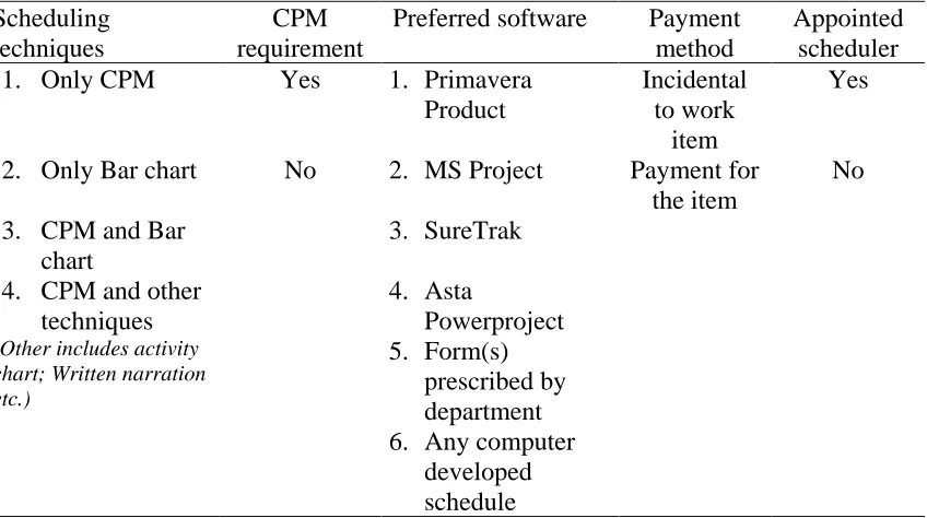
scheduling and requirement of appointed scheduler. The categories and unique values to

measure current practices from the survey of standard specifications are presented in Table

2.1.

Rowings (Rowings, Harmelink, & Rahbar, 1993) conducted a statewide survey of

the state DOTs to gather information of the scheduling practices. Thirty-six (36) DOTs

(26)

Calculation of project duration was conducted by experience, type, size of the project

(44%), past history of the projects (22%) and only 4% used CPM for the calculation.

Forty-seven (47%) responded that DOTs do not require a schedule specification. The two most

popular method of scheduling at that time were CPM and bar charts. In regard to

information loading with schedules, most of the DOTs did not request any cost or resource

loaded schedules.

Table 2.1 Focus groups for standard specifications for construction of DOT

Scheduling techniques

CPM requirement

Preferred software Payment method

Appointed scheduler

1. Only CPM Yes 1. Primavera

Product

Incidental to work

item

Yes

2. Only Bar chart No 2. MS Project Payment for the item

No

3. CPM and Bar chart

3. SureTrak

4. CPM and other techniques (Other includes activity chart; Written narration etc.) 4. Asta Powerproject 5. Form(s) prescribed by department 6. Any computer

developed schedule

The survey results of the standard specifications of each DOT is presented in

Appendix-A. This reveals that most of the DOTs require scheduling in most of their

projects. The level of scheduling may differ from state to state. For example, California

DOT requires three levels of scheduling depending upon the workings day and bid amount

of the projects. In all cases it requires a CPM schedule but the specifications are different

(27)

Depending upon the level of effort for scheduling DOTs use different scheduling

techniques. Most common techniques employed are bar charts and CPM. Other techniques

include written narrative, activity chart, any network diagram etc. Some DOTs also use

customized charts. For example, Texas DOT uses TxDOT standard spec item 8.5 for

monitoring projects.

In case of scheduling tools for CPM schedules, bar charts and CPM are most

common among the state DOTs. Some DOTs also require written narrative along with

these schedules, for example Kentucky DOT.

Payment for schedules are important parameter for measuring whether the CPM

schedules extensively used in the project or it is just a specification requirement. The state

DOTs most often include the payment for schedule as incidental to any work item. But

some DOTs explicitly pay for CPM scheduling. Some DOTs request a dedicated scheduler

for a project. This indicates the emphasize of the that DOT on CPM scheduling.

2.5 Chapter Summary

Project management literature have examined numerous causes and effects of

project delay. The use, advantages, disadvantages, and adaptation of CPM scheduling in

project management have also been studied. Most of these results are from the surveys of

owners, contractors, and state DOTs. But to the authors knowledge, no study has

investigated the use of Critical Path Method (CPM) schedules as a factor in on-time project

(28)

`CHAPTER 3: METHODOLOGY

3.1 Introduction

This chapter discusses the framework and methods used for analyzing the impact

of time overrun on the transportation projects. The methodology includes selection of

independent and dependent variable, preliminary descriptive statistics, chi-square test of

independence and two sample t-tests. It also discusses the method of conducting online

questionnaire survey to find out the impact of using CPM in projects.

3.2 Selection of Variables

To find the general trend in the data, a graphical trend analysis of the datasets for

the study is conducted. Project type, project size, project duration, and project location are

the independent variables and the time delay is considered as dependent variable. The

variable project type and project location were already categorized in the provided datasets.

The independent variable project size was categorized into three levels: small, medium,

and high. The other independent variable project duration was also categorized into three

groups: short, medium, and long. The details of categorizing the data by project size and

(29)

3.3 Descriptive Statistics and Statistical Analysis

The study aims to find out the impact of the CPM method of scheduling on time

delay of transportation projects. The descriptive analysis of the datasets reveals insights on

this objective. Simple descriptive graphs are used to characterize the data by independent

variables. Single and grouped bar plots of independent variables and frequency table

provide information to understand the data. In order to measure the relative significance of

independent variables descriptive figures such as grouped bar plots are used.

The statistical analysis is focused on determining two aspects of the data. The first

one is to examine the relationship of the variables. The second one is to determine the

difference in statistics (i.e. mean) from two populations. The Chi-square test of

independence is used to examine the relationships between variables and t-test is used to

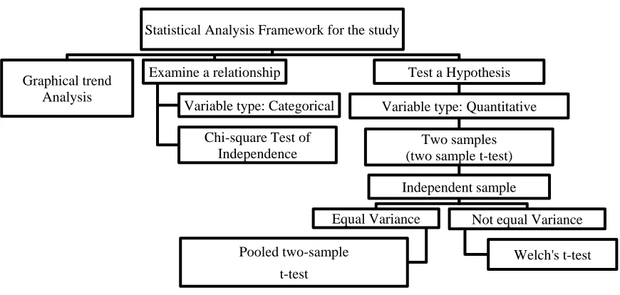
measure the difference in statistics from two samples. The overall framework of the

statistical analysis is shown in Figure 3.1

Figure 3.1 Statistical Analysis framework for the study

Statistical Analysis Framework for the study

Graphical trend Analysis

Examine a relationship

Variable type: Categorical

Chi-square Test of Independence

Test a Hypothesis

Variable type: Quantitative

Two samples (two sample t-test)

Independent sample

Equal Variance

Pooled two-sample t-test

Not equal Variance

(30)

3.3.1 Chi-square test of independence

Chi-square test of independence is used to examine the relationship between

categorical variables. Chi-square test (also known as Pearson Chi-square test) is one of the

most commonly used non-parametric test. The advantage of using a non-parametric test

lies in its assumptions. The assumptions for the Chi-square test are:

• Distribution of the sample data does not follow any specific distribution

(distribution free test).

• Sample data is collected from two categorical variables (i.e. sample data can

be distributed into distinct categories).

• The data in distinct categories should be in frequencies or counts.

• The categories of variables are mutually exclusive.

• The frequency of expected value in any cell of the contingency table of

categories should be 5 or more in at least eighty percent of the cells. In

addition to that, expected value in any cell should not be less that one.

A Chi-square test of independence is conducted by determining the distinct

category of variables for the test. The count or the frequency from the sample data are

divided into distinct categories of variables. Thus, a contingency table of observed values

is constructed from the sample data. The frequency or count on each cell of the contingency

table should follow the assumption of the Chi-square test state above. Then Chi-square test

is performed to determine if the categorical variables are related (i.e. associated) to each

other. The hypothesis tested in the Chi-square test of independence is as follows:

(31)

𝐻_𝑎: 𝐼𝑛 𝑡ℎ𝑒 𝑝𝑜𝑝𝑢𝑙𝑎𝑡𝑖𝑜𝑛, 𝑡ℎ𝑒𝑟𝑒 𝑖𝑠 𝑟𝑒𝑙𝑎𝑡𝑖𝑜𝑛𝑠ℎ𝑖𝑝 𝑏𝑒𝑡𝑤𝑒𝑒𝑛 𝑡ℎ𝑒 𝑐𝑎𝑡𝑒𝑔𝑜𝑟𝑖𝑐𝑎𝑙 𝑣𝑎𝑟𝑖𝑎𝑏𝑙𝑒𝑠.

To perform this test, first the two categorical variables are summarized in the form

of a contingency table as illustrated below

Second categorical variable First categorical

variable

1 . j Total

1 C11 . . R1

I . . . Ri

Total C1 . Cn n

The Chi-square test statistics is used to test the hypothesis. The formula to calculate

the chi-square test statistics is:

The 2 test statistic is calculated as follows (25).



    r i c j ij ij ij E ) E O ( 1 1 2 2  ₍₁₎ where,  2

 the test statistic



ij

O the observed count in cell (i, j)



ij

E the expected count in cell (i, j)

r = number of rows c = number of columns

The expected count in each cell is calculated as follows.

n C R

Eij  i j

(2)

where,

Rj and Ci are the row and column totals, respectively.

The degree of freedom is calculated using the following formula:

(32)

The chi-square test statistics finds the answer to the question whether the expected

value differs significantly from our observed value. For the decision making on the null

hypothesis a level of significance (α) is set and p-value is calculated from the chi-square

statistics by the formula P(𝜒2> 𝜒2∗) with degrees of freedom = (number of rows -

1)*(number of columns - 1). If the p-value is less than ‘α’ the null hypothesis is rejected.

The chi-square test is conducted to find if there is any association between the

depended variable (i.e. delay, cost overrun) and the use of CPM for schedules. Both the

variable is treated as binary variables. For example, the binary variable ‘delay’ is classified

as whether there is a delay (defined as ‘1’) or not (defined as ’0’). Again, for use of CPM

for schedules, whether CPM schedules used for the project or not. Two-way contingency

table is created using the two categorical variables. The null hypothesis tested is that there

is no relationship between dependent variable and the use of CPM for schedules. The test

is conducted for each independent variable (project type, project size, project location).

The results of Chi-square test of independence are presented in Appendix-B, Table 4.8.

3.3.2 t-test

The t-test is conducted to compare two means of independent variable to find out

whether these means are significantly different from each other. This test is also known as

two sample t-test. The assumptions of two sample t-test are:

• The data is continuous.

• The data follows normal probability distribution.

• The two samples are independent.

(33)

The assumption of variance in the two-sample t-test determines which t-test to use

for the comparison of the means of the samples. If the variance of the two populations are

equal (Homogeneous variances) pooled two-sample t-test is used. If the variances are not

equal (Heterogeneous variances) Welch’s two sample t-test is used.

The two independent samples are taken for each independent variable. To test the

homogeneity of variance the F-test for variance is used to test the homogeneity of variance

of the samples. The hypothesis for the F-test is:

𝐻₀: 𝑇ℎ𝑒 𝑣𝑎𝑟𝑖𝑎𝑛𝑐𝑒𝑠 𝑜𝑓 𝑡ℎ𝑒 𝑡𝑤𝑜 𝑝𝑜𝑝𝑢𝑙𝑎𝑡𝑖𝑜𝑛𝑠 𝑎𝑟𝑒 𝑒𝑞𝑢𝑎𝑙. ( 𝜎₁2 _{= 𝜎}

22)

𝐻_𝑎: 𝑇ℎ𝑒 𝑣𝑎𝑟𝑖𝑎𝑛𝑐𝑒𝑠 𝑜𝑓 𝑡ℎ𝑒 𝑡𝑤𝑜 𝑝𝑜𝑝𝑢𝑙𝑎𝑡𝑖𝑜𝑛𝑠 𝑎𝑟𝑒 𝑛𝑜𝑡 𝑒𝑞𝑢𝑎𝑙. ( 𝜎₁2 ≠ 𝜎₂2)

The result from the F-test for homogeneity indicates whether to conduct the pooled two

sample t-test or Welch’s t-test. The null hypothesis tested in both the cases is as follows:

𝐻₀: 𝑇ℎ𝑒𝑟𝑒 𝑖𝑠 𝑛𝑜 𝑑𝑖𝑓𝑓𝑒𝑟𝑒𝑛𝑐𝑒 𝑖𝑛 𝑚𝑒𝑎𝑛𝑠 𝑜𝑓𝑡ℎ𝑒 𝑡𝑤𝑜 𝑠𝑎𝑚𝑝𝑙𝑒𝑠 ( µ₁ = µ₂)

𝐻_𝑎: 𝑇ℎ𝑒𝑟𝑒 𝑖𝑠 𝑑𝑖𝑓𝑓𝑒𝑟𝑒𝑛𝑐𝑒 𝑖𝑛 𝑚𝑒𝑎𝑛𝑠 𝑜𝑓𝑡ℎ𝑒 𝑡𝑤𝑜 𝑠𝑎𝑚𝑝𝑙𝑒𝑠 ( µ₁ ≠ µ₂)

The equation of test statistics depends upon which t-test is conducted. The equation for test

statistic of the pooled sample t-test is:

𝑡∗ = 𝑥̅1− 𝑥̅2 𝑠_𝑝√1

𝑛₁+ 1 𝑛₂

Where, 𝑥̅₁ = mean of sample 1

𝑥̅₁ = mean of sample 2

𝑛₁ = sample size of sample 1

𝑛1 = sample size of sample 2

𝑠_𝑝 = Common standard deviation = √(𝑛1−1)𝑠1

2_+(𝑛 2−1)𝑠22

(34)

𝑠12= variance of sample 1

𝑠₂2= variance of sample 2

𝑑𝑓 = degrees of freedom = 𝑛₁+ 𝑛₂− 2

The equation for test statistics of Welch’s t-test and the degrees of freedom is

slightly different form the above method and is as follows:

𝑡∗ = 𝑥̅1− 𝑥̅2 √_𝑛1

1+

1 𝑛₂

With 𝑑𝑓 = degrees of freedom = _(𝑛 (𝑛1−1).(𝑛2−1)

2−1).𝐶2 +(1−𝐶)2(𝑛1−1) and 𝐶 =

𝑠₁2/𝑛₁

𝑛12 𝑛1+

𝑛22 𝑛2

The test statistics finds the answer to the question whether the means of sample 1

significantly differs from the mean of sample 2. For the decision making on the null

hypothesis a level of significance (α) is set and p-value is calculated from the test statistics

by the formula P (𝑡 >𝑡∗). The degrees of freedom to calculate the p-value is associated the

type of two sample t-test is conducted on the samples. If the p-value is less than ‘α’ the

null hypothesis is rejected. Generally, in engineering application the ‘α’ value is set to 0.05

for comparison of means of samples using two sample t-test.

The t-test is used to find out whether the depended variable (i.e. time delay, cost

overrun) significantly differed by the use of CPM schedules. The two samples were taken

from the unscheduled projects and projects scheduled by CPM method. Then the samples

were categorized by independent variable (i.e. project type, project size and project

location). The dependent variables were quantitative variables acquired from the

(35)

dependent variable when using CPM method for scheduling the projects. The results of

t-test presented in Appendix-A,Table 4.9, Table 4.11.

3.4 Survey of Use of CPM

The aim of the survey is to understand the methods used by the state agencies to

manage time delay of their projects. The survey was conducted in two steps. The first step

was to conduct online survey on the standard specifications for construction of each agency

to find out the current practices of their project management. The second step was a

questionnaire survey to acquire information on the effectiveness of Critical Path Method

(CPM) for scheduling. In addition to these steps, phone interviews of selected DOT

personnel managing projects were conducted to better understand the ins and outs of the

CPM use in practice.

3.4.1 Survey methodology

The online questionnaire survey was conducted to find the effectiveness of CPM

schedules for managing time delay of the projects. The purpose of the survey was to gather

information about selection criteria for CPM schedule for projects, contractual

requirements of CPM, preferred software, evaluation of contractor on CPM use, impact of

CPM schedules on project time extension, and different practices and approaches of project

management in transportation projects. The targeted participants of the survey were the

DOT personals, the Resident Engineers and contractors working on DOT projects. Online

questionnaire was created to conduct the survey for each category of participants.

Three separate online surveys were created for DOT personnel, Resident

(36)

information from the participants to meet the study and were distributed to other DOT

personnel, RCEs and contractors by SCDOT.

Table 3.1 Topic focused on the survey for DOT headquarter personnel, Resident Construction Engineer and Contractors

Topic focused on the survey DOT headquarter

personnel

Resident Construction

Engineer

Contractors

Scheduling technique employed/preferred

Q2, Q9 Q6

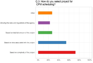
Selection of projects for CPM schedule Q3 Q2

Contract requirements / specifications of CPM scheduling

Q4, Q5 Q2

Scheduling software used/preferred Q6, Q11, Q12, Q13,

Decision making based on CPM schedules

Q3 Q4

Storage and Access of schedule database Q8, Q14, Q17

Effort made to follow CPM schedule Q4

Use of CPM schedule (planning, claim analysis, revisions of CPM etc.)

Q15, Q16 Q5, Q10 Q3, Q7, Q8

Project extension / Delay associated with CPM schedule

Q6, Q7, Q8, Q9

Schedulers requirements and tasks Q9, Q10,

Q11

Cost of CPM application Q5

Value of CPM for success of the company

Q12

The breakdown of the questions in the survey for DOT personnel, resident

engineers and contractors are shown in Table 3.1. There were seventeen questions for each

(37)

Contract specifications for CPM, (3) Scheduling techniques use, (4) Scheduling software

preference, (5) Scheduling database storage and access, and (6) Different usages of CPM

schedule.

For resident engineers, there were ten questions which focused on five areas: (1)

Selection of projects for CPM schedule, (2) Decision making using CPM schedule, (3)

Different usages of CPM schedule, (4). Delay associated with CPM schedule, and (5)

Assessment of contractors’ effort. The survey questionnaire for contractors includes

eleven questions to focus on (1) Contract specification for CPM, (2) Scheduling software

preference, (3) Decision making using CPM schedule, (4) Different usages of CPM

schedule, (5) Scheduler appointment and tasks, and (6) Cost and success of CPM use areas.

The first question of each survey is excluded in the survey matrix of Table 3.2 because it

contains information about respondent’s identity.

The participants of the survey responded to the online survey through web-based

survey tool, Google Forms. The survey is shown in Appendix-C And the results of analysis

are discussed in chapter 4 and 5.

3.4.2 Phone Interviews

Phone interviews were planned for other DOTs to verify information and

understand the schedule practices in other States. The results from the survey of DOTs of

their standard specifications and respond from the online questionnaire survey were

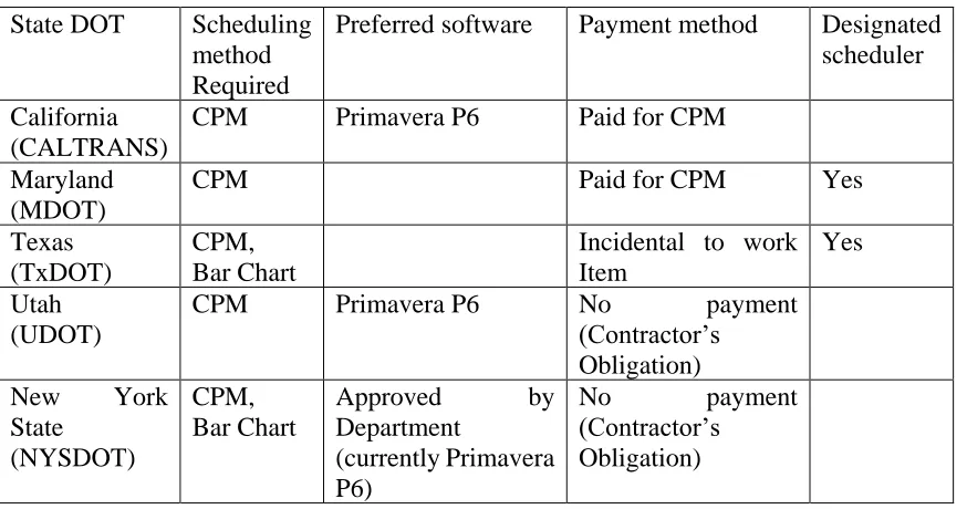
analyzed in order to select five state DOTs for phone interview. These selected DOTs for

(38)

indication of good and effective practices of CPM schedule for their projects. Table 3.3

shows the criteria used for selection from standard specifications.

Table 3.2: Lists of DOTs for phone interviews

State DOT Scheduling method Required

Preferred software Payment method Designated scheduler

California (CALTRANS)

CPM Primavera P6 Paid for CPM

Maryland (MDOT)

CPM Paid for CPM Yes

Texas (TxDOT)

CPM, Bar Chart

Incidental to work Item

Yes

Utah (UDOT)

CPM Primavera P6 No payment

(Contractor’s Obligation) New York

State (NYSDOT)

CPM, Bar Chart

Approved by

Department

(currently Primavera P6)

No payment

(Contractor’s Obligation)

Among the five state DOTs, three of them responded to our online survey. These

DOTs provided interesting response regarding selection of CPM schedule to use in their

projects and use of CPM schedule for different complexity and duration levels.

3.5 Data Description

All the data regarding projects for analysis of schedule impact on delay were

collected from the information provided by the SCDOT. The timeframe of the projects is

approximately eight years: projects let after February 2007 to June 2015. All the projects

reached substantial completion data within this timeframe. There were 2,097 projects in

(39)

SCDOT uses two types of software for the purpose of project management. The

AASHTOWARE Project SiteManager® computer application is used to manage

information regarding contracts. The dataset contains general information of SCDOT

projects, change order information, Daily Work Report (DWR) and item used in projects.

The data for time overrun analysis is recorded in the general information table of the

provided dataset. The SiteManager dataset provided by SCDOT is in Microsoft Access®

format. The codes used in the dataset are indicated in Table 3.3.

Table 3.3 Raw project data description in SiteManager provided by SCDOT

Variable Name Description

Information type

CONT_ID Unique code identifying each project Project

FED_ST_PRJ_NBR

Unique code for funding management purposes

Project

LEV3_OFFICE_NBR Engineering district that manages the project Project

LEV4_OFFICE_NBR

Resident Construction Engineer (RCE) office

Project

VEND_ID ID for prime contractor Project

TOT_BID_AMT Original bidding amount for the project Cost

NET_C_O_AMT Total change order amount Cost

Total_Paid Total amount paid Cost

TTBID TOT_BID_AMT plus NET_C_O_AMT Cost

NTP_Date Notice to proceed date Time/Dates

Adj_Comp_Date

Adjusted completion date

(original completion date plus time change order)

Time/Dates

CompDate Substantial completion date Time/Dates

Letting_Date Date the project was let Time/Dates

WRK_T

Type of project (i.e. Bridge, surfacing, painting etc.)

Project

ORGC_Date

Original completion date when the project was let

Time/Dates

DESC1 Brief description of the project Project

(40)

From Table 3.3 four types of information (e.g. project related, time related, cost

related, and project location related) for a project were separated from the database. The

information type and their related fields is also shown in Table 3.3.

Time related information includes letting date, notice to proceed date, original and

adjusted completion date and substantial completion date for each project. The total bid

amount and net change order amount data were retrieved from the dataset for cost related

analysis. For geographical information of the projects, SCDOT districts were extracted

from the database. There are seven SCDOT districts which are marked with the numbers

from 1 to 7 in Figure 3.2. These district numbers are provided in the location information

field (LEV3_OFFICE_NBR) to retrieve the geographical information of the projects.

Figure 3.2 SCDOT engineering districts

(Source:http://www.scdot.org/inside/engineering_directory.aspx accessed on 25 March, 2017)

There is a total of 2,097 projects in the SiteManager database, which are divided

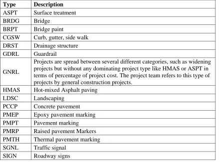
into 16 different project types defined in Table 3.4. The type of project information is

(41)

Table 3.4 Description of different types of projects in the SiteManager database

Type Description ASPT Surface treatment BRDG Bridge

BRPT Bridge paint

CGSW Curb, gutter, side walk DRST Drainage structure GDRL Guardrail

GNRL

Projects are spread between several different categories, such as widening projects but without any dominating project type like HMAS or ASPT in terms of percentage of project cost. The project team refers to this type of projects by general construction projects.

HMAS Hot-mixed Asphalt paving LDSC Landscaping

PCCP Concrete pavement PMEP Epoxy pavement marking PMPT Pavement marking

PMRP Raised pavement Markers PMTH Thermal pavement marking SGNL Traffic signal

SIGN Roadway signs

The primavera software is used by the SCDOT for planning, managing and

executing its projects. The primavera database contains information regarding Critical Path

Method (CPM) schedules of the project. The “OBSPROJ” table contains information

regarding the EPS structure and the schematic diagram of different levels of EPS is shown

in Figure 3.3. The Enterprise Project Structure (EPS) shows that all the projects in

Primavera are contained under Resident Construction Engineer (RCE) level.

The Primavera database was provided in a SQL format. The “PROJECT” table of

(42)

“PROJWBS” table contains each of the projects in “PROJECT” table with additional

information of update.

Figure 3.3 Enterprise Project Structure of Primavera database

3.5.1 Database Development

The extracted information from the SiteManager and Primavera database are

merged together to produce a completely new database for analysis. The SiteManager and

Primavera datasets were joined using the unique project identifier “CONT_ID” in

SiteManager and the “proj_short_name” field in the Primavera table “dbo_PROJECT”.

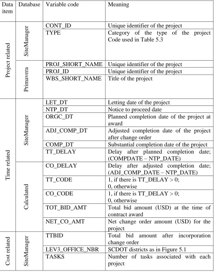
The data items in the database are listed in Table 3.5.

For the analysis of project delay following variables are used:

• CO_Delay - Time delay (in days) measured in terms of number days beyond adjusted completion date, only for projects with a CO_delay > 0

• TT_Delay - Time delay (in days) measured in terms of number of days beyond original completion date, only for projects with a TT_delay > 0

SCDOT Schedules

SCDOT Districts

Resident Construction Engineer (RCE)

(43)

Table 3.5 Database development and variables calculated

Data item

Database Variable code Meaning

Proj

ec

t r

elated Sit

eManager

CONT_ID Unique identifier of the project

TYPE Category of the type of the project Code used in Table 5.3

Prim

av

era

PROJ_SHORT_NAME Unique identifier of the project PROJ_ID Unique identifier of the project WBS_SHORT_NAME Title of the project

Time

rela

ted

Sit

eManager

LET_DT Letting date of the project NTP_DT Notice to proceed date

ORGC_DT Planned completion date of the project at award

ADJ_COMP_DT Adjusted completion date of the project after change order

COMP_DT Substantial completion date of the project TT_DELAY Delay after planned completion date;

(COMPDATE – NTP_DATE)

Calcul

ated

CO_DELAY Delay after adjusted completion date; (ADJ_COMP_DATE – NTP_DATE) TT_CODE 1, if there is TT_DELAY > 0;

0, otherwise

CO_CODE 1, if there is TT_DELAY > 0; 0, otherwise

TOT_BID_AMT Total bid amount (USD) at the time of contract award

NET_CO_AMT Net change order amount (USD) for the project

Cost r

elated

Sit

eManage

r TTBID Total bid amount after incorporation change order

LEV3_OFFICE_NBR SCDOT districts as in Figure 5.1

(44)

Locat

ion

rel

ated

Sit

eManager

SSP_CODE 1, if there is payment item for schedule; 0, otherwise

Schedule

rel

ate

d

Calcul

ated

SSPRIM_CODE 1, if the project has a real schedule in Primavera;

0, otherwise

Sit

eManager

SST_CODE 1, if there the has an entry in Primavera for schedule;

0, otherwise

The Primavera database contains projects that do not have a CPM schedule.

Observations from the “OBS” table in the Primavera database show that under each Resident Engineer (RE), there are some projects that are marked as “No CPM”. Also, some

of the project titles (WBS_SHORT_NAME) indicate that these projects do not have a CPM

schedule. These projects are identified by using the following criteria: -

i. The projects contained in the “No CPM” or “No CPM Reqd” level in the

Primavera database.

ii. Indication of a non-real CPM schedule activities: Projects that have only

“payout” or “cash flow only” or “estimate only” activities.

iii. Indication of a non CPM schedule: The title of the project (WBS_NAME

in “PROJWBS” table) contains phrases: “Non CPM” or “non cpm schedule” or “NO CPM Required”.

The above criteria are used to refine SST projects. Projects that fall into the above

criteria are excluded from the SST projects and then further categorized all the projects as

follows: -

(45)

• SSNULL - all the projects in SiteManager that are not SSPRIM.

To measure the effectiveness of the use of CPM on the delay of SCDOT projects

in terms of project size, the projects are categorized into three groups by total contract bid

amount (in USD in the corresponding year of the project in the analysis period):

• Small projects: Total contract bid amount between $0 to $ 360,000.

• Medium projects: Total contract bid amount between $360,000 to $1,000,000.

• Large projects: Total contract bid amount greater than $1,000,000.

Again, to measure the effectiveness of the use of CPM on the delay of SCDOT

projects in terms of project duration, the projects are categorized into three groups by

original duration of the projects (in months):

• Short projects: original duration of the project less than 6 months

• Medium projects: original duration of the project between 6 to 12 months • Long projects: original duration of the project more than 12 months (1 year)

3.6 Chapter Summary

This chapter discussed the framework, methods and underlying assumptions of

statistical analysis to understand the impact of use of CPM technique in projects for project

delay. The methodology used in statistical analysis included examining relationship of

categorical variables by Chi-square test of independence and hypothesis test by students’

t-test. In addition to that, the process of two-step surveys and phone interviews are also

discussed. First step of survey was conducted to gather information from standard

(46)

managing their projects. Second step was to conduct an online survey of DOT personnel,

Resident Construction Engineers and contractors about the use of CPM in their projects.

Phone interviews were also conducted for five state DOT personnel to gather information

(47)

CHAPTER 4: FINDINGS

4.1 Introduction

This chapter describes the findings obtained from online questionnaire surveys and

the statistical analysis on transportation projects from SCDOT. It provides the basic

information describing general characteristics of the project data obtained from

SiteManager and Primavera database. A detailed description of time delay classified by

various categories used in the statistical analysis gives an explicit overview of the variable.

The dependent variable, time delay, is expressed both in terms of original completion date

and adjusted completion date. The chapter also presents the survey results from the online

questionnaire surveys. Survey information reveals the viewpoint of the survey participants

on CPM method of scheduling in the transportation projects.

4.2 Descriptive Statistics

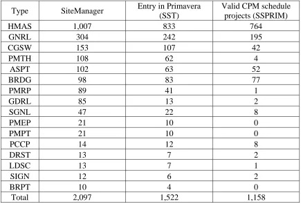
Table 4.1 shows the distribution of projects by project types. It shows that the

majority of the projects in the SiteManager database are either HMAS (48%) or GNRL

(14.5%). Table 4.1 also shows that in the Primavera database slightly more than half of

the projects have a CPM schedules (SSPRIM: 55.22%). The paint and marking projects

(BRPT, PMEP, PMPT, PMRP, and PMTH) and sign and signal projects (SGNL, SIGN)

do not generally use CPM. This is also true for other project types such as guardrail

(48)

Table 4.1, it can be concluded that certain types of projects are more likely to have a CPM

schedule.

Table 4.1: Distribution of SiteManager Projects, SST Projects and SSPRIM Projects by Project Types

Type SiteManager Entry in Primavera (SST)

Valid CPM schedule projects (SSPRIM)

HMAS 1,007 833 764

GNRL 304 242 195

CGSW 153 107 42

PMTH 108 62 4

ASPT 102 63 52

BRDG 98 83 77

PMRP 89 41 1

GDRL 85 13 2

SGNL 47 22 8

PMEP 21 10 0

PMPT 21 10 0

PCCP 14 12 8

DRST 13 7 2

LDSC 13 7 1

SIGN 12 6 2

BRPT 10 4 0

Total 2,097 1,522 1,158

Table 4.2 presents the distribution of projects by SCDOT districts (3 projects in the

data were not assigned a district). The average number of projects in each district is 299.

The district with most number of projects is district 5 with 352 projects. The number of

projects for each district range from 250 to 352. It can be concluded that the number of

projects is reasonably uniform across districts. All the districts use CPM schedules for more

than half of its projects except for District 7. The district that uses CPM schedules for

majority of their projects than other districts is District 2 (174 out of 287: 60.6%) followed

(49)

Table 4.2 Distribution of Projects by Project SCDOT districts

Districts Total number of Projects Total number of SSPRIM Projects

1 333 193

2 287 174

3 283 149

4 289 168

5 352 209

6 300 157

7 250 108

Total 2,094 1,158

Table 4.3 shows the distribution of the projects by project size (large, medium and

small). Each group contains about the same number of projects. The last column in Table

4.3 shows the number of scheduled projects in each category.

Table 4.3 Distribution of Projects by Project Size Groups

Project size Groups Total number of Projects Total number of SSPRIM Projects

Small Projects 702 206

Medium Projects 670 382

Large Projects 725 570

Total 2,097 1,158

Table 4.4 shows the distribution of projects by project duration. Long projects have

larger fraction (286 out of 439: 65.2%) of projects than other two types of projects (short:

43.41% and medium: 55.2%).

Table 4.4 Distribution of Projects by Project Duration Groups

Project duration Groups Total number of Projects

Total number of SSPRIM Projects

Short Projects 364 158

Medium Projects 1,294 714

Long Projects 439 286

(50)

4.3 Impact of CPM Schedule on Project Delay

Using the transportation project data described above, the relationship between

project delay and use of CPM schedules are evaluated. In addition to using the TT_Delay

and CO_Delay variables for delay analysis, the following variables are also used to

measure project delay:

• nCO_Delay – Number of projects with a CO_Delay delay greater than zero.

• nTT_Delay – Number of projects with a TT_Delay delay greater than zero.

Table 4.5 Impact of Using a Critical Path Method (CPM) Schedule on Project Delays by Project Type

Project Type

Total number of

projects

Number of projects delayed after original completion date

(nTT_Delay)

Number of projects delayed after adjusted completion date

(nCO_Delay) Delayed SSPRIM Delayed projects Delayed SSPRIM Delayed projects

ASPT 102 18 38 10 20

BRDG 98 48 58 11 13

BRPT 10 0 5 0 1

CGSW 153 19 64 6 23

DRST 13 1 6 0 3

GDRL 85 2 63 0 3

GNRL 304 108 161 27 39

HMAS 1,007 423 506 113 153

LDSC 13 1 10 0 0

PCCP 14 2 6 0 0

PMEP 21 0 11 0 9

PMPT 21 0 6 0 2

PMRP 89 0 35 0 14

PMTH 108 1 69 0 32

SGNL 47 5 29 1 5

SIGN 12 1 8 0 2

Total 2,097 629 1,075 168 319

(51)

Table 4.5 shows the total number of SSPRIM projects that were delayed versus the

total number of projects that were delayed in terms of nTT_Delay and nCO_delay,

respectively. The results indicate that more than half (nTT_Delay: 629 out of 1,075,

58.51% and nCO_Delay: 168 out of 319, 52.66%) of the delayed projects have a CPM

schedule. The results also indicate that fewer scheduled projects have delay after

considering the impact of change orders.

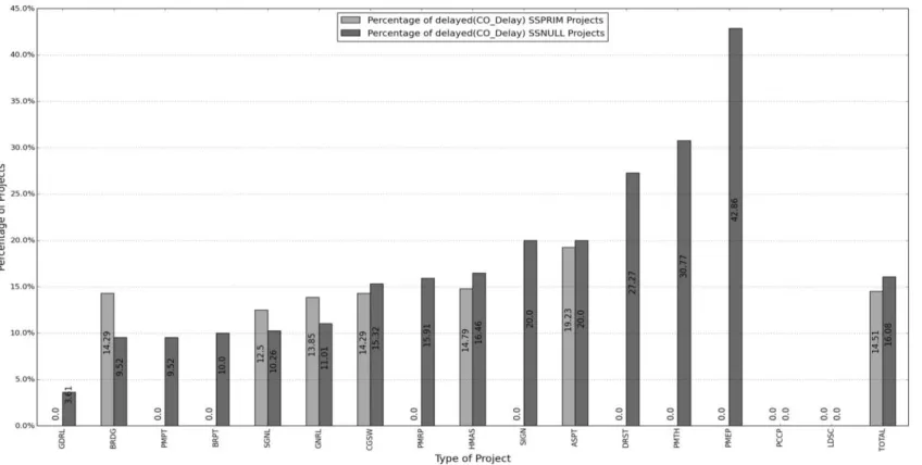
Figure 4.1 and Figure 4.2 show the impact of having a schedule on the risk of

project delay. Figure 4.1 shows that in the dataset, having a schedule was not effective in

reducing the fraction of delayed projects for most project types. In fact, the project types

that have a significant number of projects (i.e. HMAS, GNRL) show a marked increase in

the fraction of delayed projects when scheduled.

Nondestructive Evaluation Of Corrosion Damage In Reinforced Concrete Aged Slab Specimen

Scholar Commons

Impact Of Critical Path Method (CPM) Of

Scheduling On On-Time Completion Of

Transportation Projects

I

C

P

M

(CPM)

S

O

-T

C

T

P

DEDICATION

ACKNOWLEDGEMENTS

ABSTRACT

TABLE OF CONTENTS

LIST OF TABLES

LIST OF FIGURES

CHAPTER 1: INTRODUCTION

CHAPTER 2: LITERATURE REVIEW

`CHAPTER 3: METHODOLOGY



CHAPTER 4: FINDINGS