Clearance gap flow: simulations by discontinuous Galerkin method
and experiments
Helena Prausov´a1,a, Ondˇrej Bubl´ık1, Jan Vimmr1, Martin Luxa2, and Jindˇrich H´ala2
1 New Technologies for the Information Society, Faculty of Applied Sciences, University of West Bohemia, Pilsen, Czech Republic
2 Institute of Thermomechanics AS CR, v.v.i., Academy of Sciences of the Czech Republic, Prague, Czech Republic
Abstract. Compressible viscous fluid flow in a narrow gap formed by two parallel plates in distance of 2 mm is investigated numerically and experimentally. Pneumatic and optical methods were used to obtain distribution of static to stagnation pressure ratio along the channel axis and interferograms including the free outflow behind the channel. Modern developing discontinuous Galerkin finite element method is implemented for numerical simu-lation of the fluid flow. The goal to make progress in knowledge of compressible viscous fluid flow characteristic phenomena in minichannels is satisfied by finding a suitable approach to this problem. Laminar, turbulent and transitional flow regime is examined and a good agreement of experimental and numerical results is achieved usingγ−Reθttransition model.
1 Introduction
Fluid flow in narrow channels and gaps of various cross-sections is a phenomenon occuring in many technical ap-plications, such as clearance gap flow in control valves of steam turbines, tip leakage flow in gas and steam tur-bines, clearance gaps in screw compressors etc. There is a need to understand fluid flow characteristic phenomena in these types of channels and be able to simulate it pro-perly. A simple straight narrow gap formed by two parallel plates is chosen as a basic simplification of these applica-tions. The distance of the plates, and hence the character-istic dimension of the channel, is varied from 1 mm to 5 mm, length of the channel is 100 mm and width also 100 mm, so that side walls don’t influnce flow in the centre of the channel. A few classifications of small channels ac-cording to their size can be considered. Following Mehen-daleet al.(2000), [1], we can classify the considered gap as a compact passage, which is a category between meso-and microchannels on one side meso-and conventional channels on the other side. Probably more used classification has been set by Kandlikar and Grande (2003), [2]. They define microchannels up to 200μm, minichannels from 200μm to 3 mm and conventional channels from 3 mm, while the characteristic dimension is diameter in case of circular tubes and the smaller dimension of cross-section in case of rectangular channels. With respect to this classification and the emphasis on the gap of 2 mm we will call the channels under investigation minichannels, with only partial overlap into conventional channels category.
The objective of this study is to examine properties of air flow in minichannels, especially turbulent/laminar regime of the flow, and simulate it properly. It is supposed to assist in future research of more complicated cases of curved or narrowing minichannels and microchannels, in which the authors are engaged for a time, [3]. The flow
a e-mail:[email protected]
regime is influenced by many aspects as properties of the fluid, velocity of the flow, roughness of the walls, outer turbulence intensity and of course dimensions of the re-gion. Computation of Reynolds number with respect to height of the channel gives values of the order of 104, which suggests turbulent regime of the flow. However, while in macrochannels the flow passes from laminar to turbulent regime for Reynolds numbers of the order of 103, in microchannels viscous effects are predominant and the flow remains laminar even for relatively high values of Reynolds number, [4]. Situation in minichannels, which stand between these two categories, needs to be further studied.
Another subject of interest in the presented work is the free jet flow behind the minichannel, where the air leaves the channel and continues into a free space. First set of experiments and numerical simulations carried out on the minichannel showed that in spite of relatively high Reynolds number the flow in the minichannel is rather la-minar, but it is obvious that the flow behind the outflow is turbulent and the unsteady phenomenons present here are influencing also the flow in the end part of the minichannel. Transition from laminar to turbulent flow regime occurs.
Experimental and numerical research of the outlined issue is done to make progress in knowledge of the com-pressible viscous fluid flow characteristic phenomena in minichannels.
2 Numerical simulation
2.1 Governing equations
To simulate the flow numerically, the problem is simpli-fied into two dimensions. Such a simplification is enabled thanks to the width of the measured channel. The fol-lowing mathematical model in dimensionless form is con-C
Owned by the authors, published by EDP Sciences, 2015
sidered. Favre-averaged system of compressible Navier-Stokes equations is written as
∂¯ ∂t +
∂( ¯u˜j) ∂xj =
0, ∂
∂t( ¯u˜i)+
∂ ∂xj
( ¯u˜iu˜j+p¯δi j)= 1
Re
∂ ∂xj
(˜ti j+τi j), ∂
∂t( ¯e˜)+
∂ ∂xj
( ¯e˜u˜j+p¯u˜j)= 1
Re
∂ ∂xj
(˜ti j+τi j)˜ui+
+κ−κ 1 μ Pr+ μt Prt ∂ ∂xj
¯ p ¯ ,
where ¯, ˜ui, ¯p, ˜eare dimensionless mass- or time-averaged values of density, velocity, pressure and energy. Mass-averaged stress tensor and Reynolds stress tensor are given by ˜ti j = 2μS¯i j, τi j = 2μtS¯i j − 23δi jk¯, where ¯Si j =
1 2
∂˜ui ∂xj +
∂uj˜ ∂xi
−1 3δi j
∂uk˜ ∂xk.
This system is completed by two-equation k-ωmodel of turbulence with cross-diffusion term according to Wilcox (2006), [5], composed by two transport equations for turbulence kinetic energykand specific dissipation rate ω, in dimensionless form written as
∂( ¯k) ∂t +
∂( ¯u˜jk) ∂xj = τi j
∂u˜i ∂xj −β
∗¯kω+
+ 1
Re
∂ ∂xj
μ+σ∗¯k ω
∂k
∂xj
,
∂( ¯ω) ∂t +
∂( ¯u˜jω) ∂xj
=αω
kτi j
∂u˜i ∂xj
−βω¯ 2+
+ 1
Re
∂ ∂xj
μ+σ¯k ω
∂ω ∂xj
+ 1
Reσd
¯ ω
∂k
∂xj ∂ω ∂xj,
wherei,j=1,2 and closure coefficients are set as
α= 13 25, β
∗=0.09, β=0.0708, σ=0.5,
σ∗= 3
5, Prt= 8 9, σd=
⎧⎪⎪ ⎨ ⎪⎪⎩0 for
∂k
∂xj∂∂ωxj ≤0, 1
8 for∂ k ∂xj∂∂ωxj >0
and turbulent viscosity is given by
μt=¯
k
˜
ω, , ω˜ =max
⎧⎪⎪ ⎪⎨ ⎪⎪⎪⎩ω,7
8
2 ¯Si jS¯i j β∗
⎫⎪⎪ ⎪⎬ ⎪⎪⎪⎭.
Joining the transport equations of the turbulence model to the system of Favre averaged compressible Navier-Stokes equations, the following system of equations is ob-tained
∂w ∂t +
2
s=1 ∂
∂xsfs(w)=
= 1
Re
2
s=1 ∂ ∂xsf
v
s(w,∇w)+ p(w,∇w), (1)
wherewis a vector of conservative variables,fs(w) are the inviscid numerical fluxes, fvs(w,∇w) are the viscid numer-ical fluxes andp(w,∇w) is a production term. The vectors
are written as
w= ⎡ ⎢⎢⎢⎢⎢ ⎢⎢⎢⎢⎢ ⎢⎢⎢⎢⎢ ⎢⎢⎢⎢⎢ ⎢⎣ ¯ ¯ u˜1 ¯ u˜2
¯ e˜ ¯ k ¯ ω ⎤ ⎥⎥⎥⎥⎥ ⎥⎥⎥⎥⎥ ⎥⎥⎥⎥⎥ ⎥⎥⎥⎥⎥ ⎥⎦
,f1(w)=
⎡ ⎢⎢⎢⎢⎢ ⎢⎢⎢⎢⎢ ⎢⎢⎢⎢⎢ ⎢⎢⎢⎢⎢ ⎢⎣ ¯ u˜1 ¯ u˜2
1+p¯ ¯ u˜1u˜2 ˜
u1( ¯e˜+p¯) ¯ u˜1k ¯ u˜1ω
⎤ ⎥⎥⎥⎥⎥ ⎥⎥⎥⎥⎥ ⎥⎥⎥⎥⎥ ⎥⎥⎥⎥⎥ ⎥⎦
,f2(w)=
⎡ ⎢⎢⎢⎢⎢ ⎢⎢⎢⎢⎢ ⎢⎢⎢⎢⎢ ⎢⎢⎢⎢⎢ ⎢⎣ ¯ u˜2 ¯ u˜1u˜2 ¯ u˜2
2+p¯ ˜
u2( ¯e˜+p¯) ¯ u˜2k ¯ u˜2ω
⎤ ⎥⎥⎥⎥⎥ ⎥⎥⎥⎥⎥ ⎥⎥⎥⎥⎥ ⎥⎥⎥⎥⎥ ⎥⎦ , fv
1(w,∇w)=
⎡ ⎢⎢⎢⎢⎢ ⎢⎢⎢⎢⎢ ⎢⎢⎢⎢⎢ ⎢⎢⎢⎢⎢ ⎢⎢⎢⎢⎢ ⎣ 0 ˜
t11+τ11 ˜
t12+τ12
2
i=1u˜i(˜ti1+τi1)+κ−κ1
μ
Pr + μt Prt
∂
∂x1 p¯
¯
μ+σ∗¯k ω
∂
k ∂x1
μ+σ¯ωk∂∂ωx
1 ⎤ ⎥⎥⎥⎥⎥ ⎥⎥⎥⎥⎥ ⎥⎥⎥⎥⎥ ⎥⎥⎥⎥⎥ ⎥⎥⎥⎥⎥ ⎦ , fv
2(w,∇w)=
⎡ ⎢⎢⎢⎢⎢ ⎢⎢⎢⎢⎢ ⎢⎢⎢⎢⎢ ⎢⎢⎢⎢⎢ ⎢⎢⎢⎢⎢ ⎣ 0 ˜
t12+τ12 ˜
t22+τ22
2
i=1u˜i(˜ti2+τi2)+κ−κ1
μ Pr + μt Prt ∂ ∂x2
p¯
¯
μ+σ∗¯k ω
∂k ∂x2
μ+σ¯ωk∂∂ωx
2 ⎤ ⎥⎥⎥⎥⎥ ⎥⎥⎥⎥⎥ ⎥⎥⎥⎥⎥ ⎥⎥⎥⎥⎥ ⎥⎥⎥⎥⎥ ⎦ ,
p(w,∇w)=
⎡ ⎢⎢⎢⎢⎢ ⎢⎢⎢⎢⎢ ⎢⎢⎢⎢⎢ ⎢⎢⎢⎢⎢ ⎢⎢⎢⎢⎣ 0 0 0 0 τi j∂∂˜uixj −β∗¯kω αω
kτi j∂∂˜uixj −βω¯ 2+Re1 ¯
ωσd
∂k
∂xs∂∂ωxs
⎤ ⎥⎥⎥⎥⎥ ⎥⎥⎥⎥⎥ ⎥⎥⎥⎥⎥ ⎥⎥⎥⎥⎥ ⎥⎥⎥⎥⎦ .
In case of modeling transition from laminar to turbu-lent flow, the Langtry and Menter’sγ−Reθtmodel, [6], [7], is used to complete the above mentioned equations. The model uses local variables and is based on two transport equations, one for intermittencyγand one for momentum thickness Reynolds number ˜Reθt, which sets the transition onset. The transport equation for intermittency in dimen-sionless form is given as
∂( ¯γ) ∂t +
∂( ¯u˜jγ) ∂xj =
Pγ−Eγ+ 1 Re
∂ ∂xj
(μ+μt)∂∂γ
xj
,
where the production and destruction terms are
Pγ =2Flength¯S¯(γFonset)1/2(1−γ),
Eγ=0.06 ¯Ωγ¯ Fturb(50γ−1), ¯
S is the strain rate magnitude and ¯Ωis the vorticity mag-nitude. Empirical correlation for the transition onsetFonset is based on vorticity Reynolds numberReνand viscosity ratioRT and is given by following relations
Reν= y¯
2S¯
μ , RT = μt μ,
Fonset1=
Reν
2.193Reθc,
Fonset2=min(max(Fonset1,F4onset1),2),
Fonset3=max
1−
R
T 2.5
3 ,0
,
whereyis the distance from the nearest wall and
Fturb=e− RT
4
4
.
The empirical transport equation for momentum thickness Reynolds number ˜Reθtcan be written as
∂( ¯Re˜θt) ∂t +
∂( ¯u˜jRe˜θt) ∂xj =
RePθt+ 1
Re
∂ ∂xj
2 (μ+μt)∂Re˜θt ∂xj
,
where the source term is defined
Pθt=0.03 ¯
t(Reθt−Re˜θt)(1−Fθt), t= 500¯U¯μ2 is the time scale and functionFθtis
Fθt=min
⎛ ⎜⎜⎜⎜⎜ ⎝max
⎛ ⎜⎜⎜⎜⎜
⎝Fwakee(− y
δ)
4
,1−
γ−1/50 1−1/50
2⎞
⎟⎟⎟⎟⎟ ⎠,1
⎞ ⎟⎟⎟⎟⎟ ⎠,
Fwake=e−(Reω/10
5)2
, Reω= ωy¯
2 μ .
The boundary layer thicknessδis computed using
δ= 500 ¯¯Ωy
U δBL, δBL =
1
Re
15 2
˜
Reθtμ ¯ U¯ ,
where ¯U is absolute value of velocity. The empirical de-pendence of parameter Reθc, the length of the transition
Flength and the transition onset Reθt on Re˜θt are used as given by Langtry and Menter (2009), [6].
The first two terms on the right-hand side in the trans-port equation for turbulence kinetic energyk(production and dissipation terms) are multiplied by intermittencyγ. While multiplying the dissipation term, the value of inter-mittency should be within 0.1 and 1. Transport equations forγandReθtare added to the system of equations given above.
2.2 Discretization
The spatial discretization of equations (1) is performed using the discontinuous Galerkin finite element method (DGFEM), [8], [9], [10].
LetTh={Ωk:Ωk∈Ω,k=1, . . . ,K}be a triangulation of the computational domainΩ∈ R2andΓ=Γint∪Γbbe the set of innerΓintand boundaryΓbedges. The solution of equations (1) is considered in the space of vector functions
Sh=Sh×Sh×Sh×Sh, where
Sh={v(x) :v(x)∈ Pq(Ωk) ifx∈Ωk, v(x)=0 ifxΩk,∀Ωk∈ Th}
andPq(Ω
k) is the space of polynomials ofq-th order at the most.
To discretize the second order derivatives using DGFEM, the auxiliary variableθr = ∂∂Wxr for the gradient is used. The system of equations (1) can be rewritten into the system of first order equations
∂w ∂t +
2
s=1 ∂
∂xsfs(w)= 1
Re
2
s=1 ∂ ∂xsf
v
s(w,θ)+p(w,θ),
θr− ∂∂w
xr =
0, r=1,2.
Multiplying this system by a test functionv∈Sh, integrat-ing it over the elementΩkand using the Green’s theorem, the following integral identity is obtained
!
Ωk ∂w
∂t ·udΩ−
!
Ωk 2
s=1 fs(w)·
∂u ∂xs
dΩ+
+
"
∂Ωk 2
s=1
fs(w)ns·udl= 1 Re " ∂Ωk 2
s=1 fv
s(w,θ)ns·udl−
1 Re ! Ωk 2
s=1 fv
s(w,θ)· ∂u ∂xs
dΩ+
!
Ωk
p(w,θ)·udΩ,
!
Ωk
θr·udΩ+
!
Ωk w· ∂u
∂xr dΩ−
"
∂Ωk
wnr·udl=0.
The key part of the method is an approximation of curve integrals. They are evaluated in the same way as it is done in the case of finite volume method. The inviscid flux is evaluated as
2
s=1
fs(w)ns≈ H(w+,w−), on Γint∈∂Ω,
2
s=1
fs(w)ns≈ H(wb,w−), on Γb∈∂Ω,
whereHis Lax-Friedrichs flux, [11],n=[n1,n2] is vector of outer normal, valuesw−resp.w+are the left resp. right limits of the vectorwon the edgeΓandwb is a boundary value ofwcomputed from boundary conditions.
Similarly, the value of viscous flux and the value of won the edge for gradient equation are evaluated using the appropriate numerical fluxes. In present paper, the ap-proximation known as local discontinuous Galerkin (LDG) method was chosen, [12].
Let wk be a part of solutionwcorresponding to con-trol elementΩkandϕk,ibei-th basis function of the space
Pq(Ωk). Themcomponentswm
k,m=1,2, ...4, of vectorwk can be expressed as a linear combination
wm k =
q
i=1 wm
k,i(t)ϕk,i(x). (2)
Inserting it into the integral identity and evaluating the vol-ume and curve integrals using the Gauss integration rules of appropriate order, the following system of ordinary dif-ferential equations is obtained
dW
dt =R(W), (3)
where vectorWconsist of coefficients of linear combina-tion (2). Taylor polynomials are chosen as the basis func-tions of the spacePq(Ωk)
ϕ0(x)=1, ϕ1(x)= x−xs, ϕ2(x)=y−ys,
wherexsandysare coordinates of element center. Time integration of equation (3) is performed using the third order Runge-Kutta method in the form
W1 =Wn+ΔtR(Wn),
W2 =3/4Wn+1/4(W1+ΔtR(W1)),
Fig. 1.The measurement facility depicted in isometric projection (without the right wall).
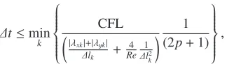
Computational efficiency of explicit schemes is directly af-fected by the maximal size of the global time step, which is limited by the CFL condition of stability
Δt≤min k
⎧⎪⎪ ⎪⎪⎪⎨ ⎪⎪⎪⎪⎪ ⎩
CFL
|λxk|+|λyk|
Δlk +
4 Re
1 Δl2
k
1
(2p+1)
⎫⎪⎪ ⎪⎪⎪⎬ ⎪⎪⎪⎪⎪ ⎭,
whereλxk,λyk is maximum wave speed in x,ydirection,
Reis Reynolds number,Δlkis diameter of control element Ωkandpis the order of polynomial approximation. A local time-stepping improvement of explicit method was imple-mented to enhance computational efficiency, [13].
Numerical simulations are performed using compu-tational environment Matlab and programming language Java. After ensuring independence of the results on the mesh resolution, the computational mesh consisting of ap-proximately 65000 nodes was used. The use of Galerkin method increases the number of degrees of freedom up to almost 200000. Capturing of effects occuring in boundary layer is accomplished by sufficient refining of the mesh near the channel walls and in the free jet.
3 Experiment
3.1 Experimental Facility
The experiments were carried out in the Aerodynamics Laboratory of the Institute of Thermomechanics AS CR, v.v.i. in Nov´y Kn´ın. The laboratory is equipped with the wind tunnel of the indraft type and intermittent operation.
For the purposes of minichannel flow examination, a special measurement facility was designed and manufac-tured. The model of the facility can be seen in Figure 1. The facility allows to perform both optical and pneumatic measurements of the flow through channels of lengthlup to 200 mm and allows smooth adjustment of the slit height
hin range from 0 to 5 mm. The proper height was set up using feeler gauge. Since sensitivity of optical methods de-pends on the width of the minichannel and also the as-sumption of the two dimensional flow needs to be satisfied reasonably, the widthwwas chosen 100 mm.
w l
h
flow
Fig. 2.Schematic view on the minichannel formed by two steel
plates with marked main dimensionsl,wandh(windows serving as a side walls are not depicted).
experimental facility
settling
chamber pipe
sliding valve
vacuum storage
flow
Fig. 3.Scheme of the set up of the experiment.
The air enters the test section directly from the labo-ratory and flows through the minichannel formed by two parallel steel plates with polished surface (upper and lower walls) and by the side walls with glass windows (Figure 2). Then the air continues to the settling chamber, where the back pressure pB is maintained during the measure-ment using the regulating slide valve downstream the set-tling chamber. The setset-tling chamber is connected to the vacuum storage by the pipe with the spherical fast-acting gate. Scheme of the set up of the experiment is depicted in Figure 3.
3.2 Methods of Measurements
The dimensions of minichannels are considerably limiting for any experimental investigation. Application of classi-cal pressure probes as well as thermoanemometric probes is problematic since the dimension of the probes might be comparable to the height of the minichannel. Use of these techniques could cause significant disturbances in exam-ined flow field, resulting in unreliability of the measured data. For the optical measurements, special care must be devoted to setting the parallelism between channel walls and the beam of the light. This is important particularly for identification of the interference fringes near the wall. Used measurement methods will be briefly described in further paragraphs.
8
8
1
,
2
÷
1
,
5
detail of the pressure tap 2,1
0,6
1,07 10×2,14
10 4×15
R8
100
flow direction
Fig. 4.Scheme of the upper wall of the minichannel of the length
100 mm with plotted positions of pressure taps and a detailed view of the pressure tap.
not influenced by those which are positioned upstream and allows denser spacing. Also the pressure in the settling chamber and the barometric pressure was measured.
For the pressure data acquisition two 16 channel pres-sure scannersPSI 9116were used. The scanner integrates 16 silicon piezoresistive pressure sensors and microproces-sor that performs a correction for senmicroproces-sor zero, span, linear-ity and thermal errors. The manufacturer guarantees sys-tem accuracy of up to±0.05% of the full scale. The con-nection between the pressure scanners and pressure taps was realised using the plastic tubes of diameter 0.5 mm and length up to 0.5 m.
Total pressure measurements were not carried out, due to the small dimensions of the channel that does not allow to use Pitot probe inside the channel for most of the inves-tigated dimensions.
The optical methods are very useful for minichannel measurements since it allows to perform the measurements without the intrusion of any probe in to the flow. It is very important because the probe dimensions might be of the same order as a characteristic dimension (height) of the minichannel, and thus an intrusion of the probe can affect the flow and bias the measurements.
Aerodynamic Laboratory in Nov´y Kn´ın is equipped with the Mach-Zehnder type interferometer. The scheme of the optical path is given in Figure 5. During the ex-position, the light from the light source goes through the monochromatic filter and field lens to make a collimated
mercury lamp
mono-chromatic filter
beam splitter
casing of the interfer-ometer
compen-sating glasses
flap spark light source
screen (camera)
test section windows mirror
beam splitter
field lens
iluminant transposi-tion elements
mirror
mirrors field
lens
Fig. 5.Schematic depiction of the light beam passing through the
Mach-Zehnder interferometer.
beam of monochromatic light. Lasers, spark light gener-ators or LED diodes can be used as a light source. In this case the spark light source was used providing suffi-cient light intensity and sufficiently short exposition time (2·10−6s) which allows to take a picture even when the flow is unsteady. The beam is then split by the beam split-ter forming a reference and a sample beam. The sample beam further goes through test section, where the mea-sured model is placed, meanwhile, the reference beam is reflected by the mirror to the upper branch of interferome-ter, where the compensating glasses are placed in order to retain the same optical path as for the sample beam. Then both sample and reference beams meet again and are re-flected to the CCD camera through some other optical ele-ments.
When there is no flow in the test section and the mirrors are adjusted exactly in line and parallel, then both beams have the same phase shift and no interference patterns can be observed on the screen (camera). This set-up is known as anInfinite-Fringe technique. During the measurement there are significant density gradients and thus gradients of index of refraction in the test section, causing the phase shift of the sample beam. If there is a phase shift between sample and reference beams, the interference patterns are formed and it is possible to take the interferogram using the digital camera.
The interference fringes visible in the interferograms represent the lines of the constant refraction index. Eval-uation of the flow parameters from the interferograms is based upon Lorentz-Lorenz equation, which relates the densityρand the absolute index of refractionnof the trans-parent medium as follows
n2−1
n2+2· 1
ρ=r, (4)
Fig. 6.Interferogram of the flow inside a minichannel of the height 2 mm and pressure ratioπ = 0.188 (the image is out-stretched in the vertical direction).
to rewrite the relation (4) into equation
r= n
2+1
n2+2·
n−1 ρ =.
2 3·
n−1
ρ , (5)
which can be simplified to Gladston-Dale relation
n−1
ρ =K, (6)
whereKis the Gladston-Dale constant.
From geometrical optics and considering assumption of negligible influence of beam curvature on the optical path length, the following relation can be derived
ρ=ρS −Ci. (7) ρS is a known reference density,i is a number of inter-ference fringe from the reinter-ference one andCis a constant involving wavelength of the used light, Gladston-Dale con-stant and width of the test sectionLt
C= λ LtK
. (8)
Knowing the density at some point of the flow field, the distribution of the density can be evaluated from interfer-ograms using equation (7). As a reference densityρS the stagnation density of the air was assumed in the entrance plane of the minichannel, i.e. the first interference fringe has a numberi=1. The example of an interferogram can be seen in Figure 6.
4 Results and discussion
4.1 Results of the experiment
At first, the experimental investigation was carried out for a minichannel of the heighth = 2 mm. Both optical and pneumatic measurements were performed for various pres-sure ratiosπ(ratio of the back pressure to stagnation pres-sure).
In Figure 7 the comparison of pressure ratio ppi
01 (ratio
of the static pressure to stagnation pressure p01) for pres-sure ratioπ=0.188 obtained using pneumatic and optical methods can be seen. It is necessary to be aware of the fact that these two methods should not provide exactly same re-sults, because for the computation of the pressure from op-tical measurements the isoentropic relation between pres-sure and density
p=p01
ρ ρ01
κ
was used, and thus the value of static pressure is lower than the one obtained using pneumatic method.
The pressure ratioπ=0.188 was chosen as a represen-tative for an illustration. For all the cases when the flow is choked the plots of pressure are very similar.
0 20 40 60 80 100
0.4 0.6 0.8 1
x(mm) pi p01
(
−
)
π=0.188 optical measurement
π=0.188 pneumatic measurement
Fig. 7.Ratio of the static pressure to stagnation pressurep01along
the minichannel axis for pressure ratioπ=0.188, obtained using pneumatic and optical methods.
0 20 40 60 80 100
0.4 0.6 0.8
x(mm) pi p01
(
−
)
h=0.5 mm
h=1 mm
h=2 mm
h=4 mm
h=5 mm
Fig. 8.Distribution of the pressure ratio pi
p01 along the minichan-nel axis for various minichanminichan-nel heights obtained from pneumatic measurements.
4.2 Numerical results in comparison with experiment
The gap of heighth=2 mm and pressure ratioπ=0.188 was chosen as a representative. First laminar and fully tur-bulent simulations were performed. Results are presented in Figure 9 in form of the pressure ratiopi/p01(static pres-sure to stagnation prespres-sure) along the minichannel axis. As can be seen from the graph, neither laminar nor fully turbulent aproach to this case is suitable and as stated in the introduction, transition from laminar to turbulent flow regime has to be simulated. In this case Figure 9 shows very good agreement of the experimental and nu-merical results, which was achieved by use of theγ−Reθt model of transition. Distribution of Mach number along the minichannel axis is displayed in Figure 10.
Fig. 9.Distribution of static to stagnation pressure ratio along the
minichannel axis for pressure ratioπ=0.188.
Fig. 10.Distribution of Mach number along the minichannel axis
for pressure ratioπ=0.188; speed of sound is achieved at about 85% of the channel length.
The air flow behind the minichannel is also a subject of interest in this study. Good agreement of the numeri-cal results with the experimental ones confirmes suitability of the used mathematical model and the chosen numerical method for the simulation. Since interference fringes are directly related to the density isolines (through relations (6), (7) and (8)), comparison of the interferograms and
computed density contour lines in Figures 11 and 12 is pos-sible. They show corresponding sequence of shock waves, which is formed in the outflow behind the minichannel.
Fig. 11.Interferogram of the flow at the end of the minichannel
and in the free outflow, for minichannel of height of 2 mm and pressure ratioπ=0.188.
Fig. 12.Density isolines obtained using the γ−Reθt model of
transition.
5 Summary
Flow conditions in the narrow gaps classified as minichan-nels have been studied both experimentally and numeri-cally. Modern developing discontinuous Galerkin finite el-ement method was implel-emented for spatial discretization of both the system of Favre averaged compressible Navier-Stokes equations and the transport equations of turbulence and transitional model. Presented results for minichannel of height 2 mm and pressure ratioπ = 0.188 show good agreement between experimental measurement and numer-ical simulation using theγ−Reθttransitional model. Pre-liminary simulations have been run for another pressure ratios and minichannel widths and will be the aim of the subsequent study, together with giving more precision to the measurements.
investigation. The most serious one is very laborious set-ting of the minichannel height and the parallelism of the walls. Even though the smallest feeler gauge used for the adjustment of the height had a thickness of 0.05 mm, the actual inaccuracies might be higher due to compliance of the whole structure. It turned out that the flow is very sen-sitive on the accuracy of the minichannel walls adjustment and its parallelism.
Acknowledgement:This work was supported by the Euro-pean Regional Development Fund (ERDF), project ”NTIS - New Technologies for the Information Society”, Euro-pean Centre of Excellence, CZ.1.05/1.1.00/02.0090, and by student project SGS-2013-036. Consultations with Prof. Jarom´ır Pˇr´ıhoda are also gratefully acknowledged.
References
1. Mehendale S. S., Jacobi A. M., Shah R. K.: Applied Mechanics Reviews53(7), (2000) 175-193.
2. Kandlikar S. G., Grande W. J.: Heat Transfer Engineer-ing24(1), (2003) 3-17.
3. Vimmr J., Kl´aˇsterka H., Hajˇzman M., Luxa M., Dvoˇr´ak R.: Journal of Thermal Science,19(4), (2010) 289 -294. 4. Kandlikar S. G., Garimella S., Li D., Colin S., King M.
R.: Heat Transfer and Fluid Flow in Minichannels and Microchannels, (Elsevier, Oxford, 2006) p. 450. 5. Wilcox D. C.: Turbulence Modeling for CFD, (DCW
Industries, La Ca˜nada, 2006), 3rdedition, p. 522. 6. Langtry R. B., Menter F. R.: AIAA Journal 47(12),
(2009) 2894-2906.
7. F¨urst J., Straka P., Pˇr´ıhoda J., ˇSimurda D.: EPJ Web of Conferences45, 01032 (2013).
8. Reed W. H., Hill T. R.: Los Alamos Scientific Labora-tory Report LA-UR-73-479, (1973).
9. Cockburn B., Shu C.-W.: Journal of Scientific Comput-ing16, (2001) 173 - 261.
10. Dolejˇs´ı V., Hol´ık M., Hozman J.: Journal of Computa-tional Physics230(11), (2011) 4176-4200.
11. Toro E. F.: Riemann Solvers and Numerical Meth-ods for Fluid Dynamics, (Springer, Heidelberg, 1999), p. 325.
12. Cockburn B., Shu C.-W.: SIAM Journal of Numerical Analysis35, (1998) 2440 - 2463.
13. Birken P., Gassner G., Haas M., Munz C.-D.: Euro-pean Congress on Computational Methods in Applied Sciences and Engineering (ECCOMAS 2012), (2012) 4334-4353.