Disentangling stellar activity from exoplanetary signals with
interferometry
Roxanne Ligi1,a, Denis Mourard1, Anne-Marie Lagrange2, Karine Perraut2, and Andrea Chiavassa1
1 Laboratoire Lagrange, UMR 7293 UNS-CNRS-OCA, Boulevard de l’Observatoire, CS 34229, 06304
NICE Cedex 4, France
2 UJF-Grenoble1/CNRS-INSU, Institut de Plan´etologie et d’Astrophysique de Grenoble, UMR 5274, Grenoble, F-38041, France
Abstract. Stellar activity can express as many forms at stellar surfaces: dark spots, convective cells, bright plages. Particularly, dark spots and bright plages add noise on photometric data or radial velocity measurements used to detect exoplanets, and thus lead to false detection or disrupt their derived parameters. Since interferometry provides a very high angular resolution, it may constitute an interesting solution to distinguish the signal of a transiting exoplanet and that of stellar activity. It has also been shown that granulation adds bias in visibility and closure phase measurements, affecting in turn the derived stellar parameters. We analyze the noises generated by dark spots on interferometric observables and compare them to exoplanet signals. We investigate the current interferometric instru-ments able to measure and disentangle these signals, and show that there is a lack in spatial resolution. We thus give a prospective of the improvements to be brought on future interferometers, which would also significantly extend the number of available targets.
1 Introduction
The discovery of the first exoplanet around a solar-type star [1] has opened up the wide field of ex-oplanet detection and characterization. The two most prolific methods used to detect exex-oplanets are the radial velocity (RV) measurements and the transit method. While the first one provides the ratio of the minimum mass of the exoplanet and the stellar mass,Mpsin(i)/M, the second one gives the ratio of their radii,Rp/R. These ratios are much amore accurate than the stellar parameters,MandR, which constitutes a limitation for exoplanet characterization. The determination of exoplanet density, composition, and habitability is only possible if exoplanet parameters are known with a sufficient ac-curacy (for example, we can estimate that 2% acac-curacy onRpis needed because it is required in some models; see, e.g., [2]). It is therefore essential to improve stellar parameters accuracy to achieve this goal. Meanwhile, stellar activity, that expresses under different forms (magnetic spots, granulation, bright plages), constitutes another limitation in exoplanet detection and characterization. It adds noise in RV measurements (see, e.g., [3]; [4]; [5]; [6]) and transit light-curves, and also on interferometric observables [7], and should thus be analyzed and quantified for a better estimate of exoplanet param-eters. We first give, in Sect. 2, a few solutions to obtain accurate stellar parameters, particularly with interferometry, and the limitations of this method. In Sect. 3, we show how interferometry could be a good solution to characterize exoplanets and distinguish it from stellar activity signals.
a e-mail:[email protected]
DOI: 10.1051/ C
Owned by the authors, published by EDP Sciences, 2015
/201
epjconf 51010 05 0
7KLVLVDQ2SHQ$FFHVVDUWLFOHGLVWULEXWHGXQGHUWKHWHUPVRIWKH&UHDWLYH&RPPRQV$WWULEXWLRQ/LFHQVHZKLFKSHUPLWV XQUHVWULFWHGXVHGLVWULEXWLRQDQGUHSURGXFWLRQLQDQ\PHGLXPSURYLGHGWKHRULJLQDOZRUNLVSURSHUO\FLWHG
2 Stellar parameters : determination and limitations
Several methods are used to estimate stellar parameters. For instance, asteroseismology allows mea-suring stellar oscillation frequencies, which gives access to stellar gravity, radius, and density through models. In particular, the stellar radius is very important both for stellar and planetary characterization, as shown in the Introduction. A more direct method to derive the stellar radius is to use interferometry, that allows measuring complex visibilities. The visibility function represents the Fourier transform of the brightness distribution of the source; this complex function is sampled by interferometric observ-ables and can be used either for recovering images of the source or to adjust model parameters to the measurements. It is decomposed into two parts: usually, we use the squared of the amplitude called the squared visibility, and its argument, called the phaseφ, described asφ=tan−1(V)
(V)
, whereand define the real and imaginary part of the complex numberV.
In the case of stars, measuring the squared visibility allows estimating their angular diameter with almost model-independent method (see, e.g., [8]). It is then used in stellar models to derive the other parameters: effective temperature, radius, mass, age.
However, current interferometers are limited to the observation of bright objects, which generally do not include transiting exoplanet host stars (see Fig. 7 in [9]). This is mainly due to insturmental bias: CoRoT andKepler were the two most important providers of exoplanets but only focused on faint stars. In general, interferometers measure visibilities in the first lobe only, or are not able to measure closure phase (CP), making the measurement of limb darkening and smaller effects, such as stellar activity effects and transiting exoplanet signals, impossible. However, due to its high angular resolution, this method could constitute a good solution to characterize exoplanets.
3 The charactarization of exoplanets and stellar activity
The codeCOMETS(code for modeling exoplanets and spots, [9]) allows measuring the complex visi-bility of a star with a transiting exoplanet, a dark magnetic spot, or both, and thus characterizing their signals on interferometric observables. The detailed methodology and calculations are presented in [9].
3.1 Minimum Baseline Length
We first estimate the Minimum Baseline Length (MBL) needed to detect a given signal caused by a transiting exoplanet or a spot in the visible wavelength (720 nm) considering several parameters and a host star of 1 mas. To that purpose, we either consider the absolute signal, that is|V2
p+−V2|>S, whereV andVp+ are the visibility modulus of the star alone and of the star with the transiting exoplanet. We calculate the MBL for signals S of 0.5%,1.0%, and 2.0% in squared visibilities, and 2◦ and 20◦in phases. This methods implies that the signal is limited by a fixed noise, which is very conservative. Another way of calculating the MBL is to consider that the signal-to-noise ratio (S/N) is photon-noise limited. This means that we calculate the MBL for a signal such as |V
2 p−V2|
V2 >
1
S/N. A
S/N of 5 corresponds to bad observing conditions and a S/N of 20 to good ones. The most important results are given in Table 1.
The longest baselines in the world currently reach 330 m and are located on the CHARA array [10]. According to this model, this is sufficient to detect a large transiting exoplanet (θp=0.09 mas) or a dark spot (that is with a low temperature,Ts=4875 K) considering absolute variations. Considering the S/N leads to the detection of smaller exoplanets and brighter spots. However, these signals are weak, and detecting an exoplanet or a spot by measuring the phases would be more realistic and feasible as the signals they cause are detectable.
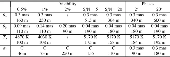
Visibility Phases
0.5% 1% 2% S/N=5 S/N=20 2◦ 20◦
θ 0.3 mas 0.3 mas / 0.3 mas 0.3 mas 0.3 mas 0.3 mas
160 m 250 m 515 m 364 m 340 m 600 m
θp 0.09 mas 0.14 mas 0.20 mas 0.04 mas 0.04 mas 0.04 mas 0.04 mas
110 m 110 m 90 m 190 m 180 m 180 m 190 m
Ts 4870 K 4030 K / 5170 K 5170 K 5170 K 5170 K
100 m 108 m 175 m 158 m 184 m 192 m
αp C C C C C 0.3 mas 0.3 mas
46m 73 m 250 m 155 110 m 90 m 180 m
Table 1: Summary of the results obtained for the MBL tests. For each tested parameter (stellar diameter θ, exoplanet diameterθp, spot temperatureTs, and exoplanet position on the stellar discαp) we list the lowest or highest value of our test for which a MBL is found and the value of the corresponding MBL (see text). C stands for constant.
MBL=(17×S0.1)×
⎛ ⎜⎜⎜⎜⎜ ⎝θθp
−
S 2
⎞ ⎟⎟⎟⎟⎟ ⎠
−1.7×S0.2
× θ 1mas
−1
× λ
720.10−9 m, (1)
whereS represents the signal to be detected ansλthe observing wavelength.
3.2 Detectability
Having long enough baselines to detect a signal does not mean that an intrument can actually do it: it depends on its sensitivity. Therefore, we have to consider the spatial frequency at which the signal caused by the exoplanet or the spot can be detected. UsingCOMETS, we computed the signal caused by an exoplanet as a function of its diameter for several spatial frequencies; in the first visibility lobe, close to the first null, and in the second lobe.
In the first visibility lobe, the signal caused by the exoplanet is weak. A 0.10 mas exoplanet causes the highest signal of 0.05%, while only a large exoplanet (∼0.20 mas) can be detected with a S/N of 20. These results are similar considering the phase: under a diameter of 0.20 mas, the signal caused by an exoplanet is below 2◦.
Small exoplanets start to be detectable close to the first null and in the second lobe. The phase seems to be more adapted to detect them: the phase signal reaches 2◦ for a∼ 0.09 mas exoplanet in the first visibility null, and for a ∼ 0.06 mas exoplanet in the second lobe. It seems possible to detect similar exoplanets in visibility measurements; for example, under good observing conditions (S/N=20), an exoplanet of∼0.06 mas could be detectable. However, condidering the absolute signal, only exoplanets larger than∼0.13 mas cause a signal of at least 0.05%.
Detecting an Earth-sized or a Neptune-sized planet is thus very difficult because instruments do not reach the needed accuracy on measurements. It should not be forgotten that phase and CP ments depend at first on the ability to measure the visibility because they are higher order measure-ments; having a phase measurement means that the visibility measurement is not too weak. Most of instruments able to measure CP can only do it in the first lobe, which is not enough to detect transiting exoplanets.
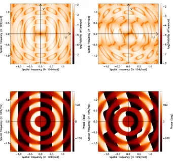
3.3 Distinguishing exoplanet and spot
Fig. 1: Map of the signal induced by an exoplanet at (0.2,0.0) mas and a spot at (0.2,0.2) mas on the stellar disc in the visibility modulus (log scale, upper panels) and the phases (bottom panels), for a 1 mas star.Left: exoplanet alone withθp =0.10 mas.Middle: exoplanet of diameterθp = 0.10 mas with a spot of diameterθs=0.10 mas.
(left), and the corresponding phases (bottom panels). The right panels show this same system with an additional dark spot of diameter 0.01 mas.
4 Conclusion
COMETSallows computing the signal caused by a transiting exoplanet and/or a spot on interferometric observables. It has been used to calculate the baseline lengths needed to detect an exoplanet or a spot, the ability of interferometers to detect such signals in terms of accuracy, and the noise generated by darks spots on exoplanet signals. We have shown that the main limitation to detect exoplanets lies in the accuracy of instruments, and that spot can mimic exoplanet signals. Distinguishing between both signals requires several observations and a significant improvement in accuracy. This is also valid to characterise Earth-sized and Neptune-sized exoplanets. Finally, the visible domain provides a better angular resolution than the infrared domain at similar baseline, and therefore appear more suitable. However, no current interferometer is able to characterize exoplanets: the visible instruments on the CHARA array, VEGA ([11]; [12]) and PAVO [13], are not accurate enough, and baselines at the VLTI are too short. Most of exoplanets detected until now are too faint to be observable with current interferometers. In the next years, new spatial missions, such as PLATO [14], TESS [16], or CHEOPS [15], will allow detecting exoplanets around bright stars, and complementary observations from the ground, especially by interferometers, will become possible.
References
1. Mayor, M. & Queloz, D. 1995, Nature, 378, 355 2. Valencia, D., et al. 2013, ApJ, 775, 10
3. Lagrange, A.M., et al. 2010, A&A, 512, A38 4. Meunier, N., et al. 2010, A&A, 512, A39 5. Boisse, I., et al. 2011, A&A, 528, A4 6. Dumusque, X., et al. 2011, A&A, 527, A82 7. Chiavassa, A., et al. 2014, A&A, 567, A115 8. Ligi, R., et al. 2012, A&A, 545, A5
9. Ligi, R., et al. 2014, A&A, in press, 2014arXiv1410.5333L
10. McAlister, H. A., et al. 2012, in Society of Photo-Optical Instrumentation Engineers (SPIE) Con-ference Series, Vol. 8445
11. Mourard, D., et al. 2009, A&A, 508, 1073
12. Ligi, R., et al. 2013, Journal of Astronomical Instrumentation, 02, 1340003
13. Ireland, M. J., et al. 2008, in Society of Photo-Optical Instrumentation Engineers (SPIE) Confer-ence Series, Vol. 7013
14. Rauer, H. & Catala, C. 2012, in EGU General Assembly Conference Abstracts, Vol. 14, 7033 15. Broeg, A., et al. 2013, in European Physical Journal Web of Conferences, Vol. 47, 3005