Power System Transient Stability Analysis Based On Interval Type-2 Fuzzy Logic Controller And Genetic Algorithms

Power System Transient Stability Analysis based on Interval

Type-2 Fuzzy Logic Controller and Genetic Algorithms

D.N. DewanganP

1

P

,PPManoj Kumar JhaP

2

P

, M. F. QureshiP

3

P

1

P

Department of Mechanical Engg., Ph.D. Scholar, Dr. C.V. Raman University,Bilaspur, India.

P

2

P

Department of Applied Mathematics, RSR Rungta College of Engg. & Tech., Raipur, India

P

3

P

Department of Electrical Engg., Govt. Polytechnic, Janjgir-Chapa, India

Abstract:

This work aims to develop a controller based on interval type-2 fuzzy logic to simulate an

automatic voltage regulator (AVR) in transient stability power system analysis. It was simulated a

one machine control to check if the interval type-2 fuzzy logic controller (IT2FLC) implementation

was possible. After which results were compared to the results obtained with the AVR itself. The

traditional type-1 Fuzzy Logic Controller (FLC) using precise type-1 fuzzy sets cannot fully handle

such uncertainties. A type-2 FLC using type-2 fuzzy sets can handle such uncertainties to produce a

better performance. However, manually designing the type-2 Membership Functions (MFs) for an

interval type-2 FLC is a difficult task. This paper will present a Genetic Algorithm (GA) based

architecture to evolve the type-2 MFs of interval type-2 FLCs used for transient stability power

system analysis.

Keywords:

Algorithms, Automatic Voltage Regulator.

1. Introduction

From the power system point of view, the excitation system must contribute for the effective

voltage control and enhancement of the system stability. It must be able to respond quickly to a

disturbance enhancing the transient stability and the small signal stability. Three principal control

systems directly affect a synchronous generator: the boiler, governor, and exciter controls.

Assuming that the generating unit has no losses. It is a reasonable assumption when total losses of

turbine and generator are compared to total output. Under this assumption all power received, as

steam must leave the generator terminals as electric power. The governor controls the steam power

amount admitted to the turbine. The excitation system controls the generated EMF of the generator

and therefore controls not only the output voltage but the power factor and current magnitude as

well. In many present-day systems the exciter is a dc generator driven by either the steam turbine

(on the same shaft as the generator) or an induction motor. An increasing number are solid-state

systems consisting of some form of rectifier or thyristor system supplied from the ac bus from an

alternator exciter. The voltage regulator is the intelligence of the system and controls the output of

modern systems the automatic voltage regulator (AVR) is a controller that senses the generator

output voltage (and sometimes the current) then initiates corrective action by changing the exciter

control in the desired direction. The speed of the AVR is of great interest in studying stability.

Because of the high inductance in the generator field winding, it is difficult to make rapid changes

in field current. This introduces a considerable lag in the control function and is one of the major

obstacles to be overcome in designing a regulating system. The purpose of this work is the

development of a interval type-2 fuzzy logic controller software (IT2FLC software) to simulate the

automatic voltage regulator (AVR) behavior.

The use of convectional automatic voltage Regulator (CAVR) in synchronous generators to

control the terminal voltage and reactive power has been the common phenomena in power systems

control. Synchronous generators are nonlinear systems which are continuously subjected to load

variations and the AVR design must cope with both normal load and fault condition of operation.

Evidently, these conditions of operation result to considerable changes in the system dynamics.

When the CAVR with fixed gain are used, the performance worsens and in some cases, introduces

negative damping and degraded system stability. So far, a lot of work has been done in synchronous

machine excitation stabilization using CAVR and controllers, all geared toward overcoming the

problems enumerated above. The short comings here is that the parameters of the controllers are

fixed and so if the system dynamics changes as a result of faults, the controller will be tuned

manually to adjust. Modern control techniques are used extensively to achieve self-tuning (ST)

control in synchronous generators. These include minimum variance (MV), generalized minimum

variance (GMV), optimal predictor and pole placement (PP). In all these ST-AVR work, additional

signals are used to improve robustness and are generally nonlinear. The MV generally gives very

lively control and can be highly sensitive to non minimum phase plant. GMV, which is more robust

and generalized, is vulnerable to unknown or varying plant dead time and can have difficulty with

d.c offsets. PP aims to locate the closed-loop poles of the system at pre-specified locations leading

to smooth controllers, but the algorithm shows numerical sensitivity when the plant model is over

parameterized. Of recent, a lot of research is going on in areas of application of soft computing

(fuzzy and neural approach) in synchronous generator controls. This work is based on interval

type-2 fuzzy logic controller (ITtype-2FLC). (ITtype-2FLC) in synchronous generator (SG) terminal voltage and

reactive power control is designed so that it has the ability to improve the performance of interval

type-2 fuzzy logic controller. The interval type-2 fuzzy logic controller is superior to conventional

AVR controllers which continue to tune the controller parameters because it will tune and to some

extent remember the values that it had tuned in the past.

The interval type-2 fuzzy logic is credited with being an adequate methodology for

designing interval type-2 fuzzy logic controller (IT2FLC) that are able to deliver a satisfactory

performance in applications where the inherent uncertainty makes it difficult to achieve good results

using traditional methods. As a result the interval type-2 fuzzy logic controller (IT2FLC) has

become a popular approach to power system transient stability control in recent years. There are

many sources of uncertainty facing the interval type-2 fuzzy logic controller (IT2FLC) for a power

system transient stability in changing and dynamic unstructured environments; we list some of them

as follows:

a. Uncertainties in inputs to the IT2FLC which translate to uncertainties in the antecedent

Membership Functions (MFs) as the sensor measurements are typically noisy and are affected by

the conditions of observation (i.e. their characteristics are changed by the environmental conditions

such as wind, sunshine, humidity, rain, etc.).

b. Uncertainties in control outputs which translate to uncertainties in the consequent MFs of

the IT2FLC. Such uncertainties can result from the change of the actuators characteristics which

can be due to wear, tear, environmental changes, etc.

d. Uncertainties associated with the use of noisy training data that could be used to learn,

tune or optimize the IT2FLC.

Recent work had proposed the use of neural based systems to learn the type-2 FLC

parameters. However, these approaches require existing data to optimize the type-2 FLC. Thus, they

are not suitable for applications where there is no or not sufficient data available to represent the

various situations faced by the IT2FLC controller. Genetic Algorithms (GAs) do not require a priori

knowledge such as a model or data but perform a search through the solution space based on natural

selection, using a specified fitness function. We did not evolve the interval type-2 FLC rule base as

it will remain the same as the interval type-1 FLC rule base. However, the FLC antecedents and

consequents will be represented by interval type-2 MFs rather than type-1 MFs.

2. Transient Stability Analysis

The first demand of electrical system reliability is to keep the synchronous generators

working in parallel and with adequate capacity to satisfy the load demand. If at any time, a

generator looses synchronism with the rest of the system, significant voltage and current fluctuation

can occur and transmission lines can be automatically removed from the system by their relays

deeply affecting the system configuration. The second demand is maintaining power system

integrity. The high voltage transmission system connects the generation sources to the load centers.

Interruption of these nets can obstruct the power flow to the load. This usually requires the power

system topology study, once almost all electrical systems are connected to each other. When a

power system under normal load condition suffers a disturbance there is synchronous machine

voltage angles rearrangement. If at each disturbance occurrence an unbalance is created between the

system generation and load, a new operation point will be established and consequently there will

be voltage angles adjustments. The system adjustment to its new operation condition is called

"transient period" and the system behavior during this period is called “dynamic performance”.

As a primitive definition, it can be said that the system oscillatory response during the

transient period, short after a disturbance, is damped and the system goes in a definite time to a new

operating condition, so the system is stable. This means that the oscillations are damped, that the

system has inherent forces which tend to reduce the oscillations. The instability in a power system

can be shown in different ways, according to its configuration and its mode of operation, but it can

also be observed without synchronism loss.

3. Automatic Voltage Regulator (AVR)

Automatic devices control generators voltages output and frequency, in order to keep them

constant according to pre-established values. These automatic devices are:

1. Automatic Voltage Regulator (AVR)

2. Governor

However any governor due to its action loop, is slower than the AVR This is associated

mainly to its final action in the turbine. The main objective of the automatic voltage regulator AVR

is to control the terminal voltage by adjusting the generators exciter voltage. The AVR must keep

track of the generator terminal voltage all the time and under any load condition, working in order

to keep the voltage within pre-established limits. Based on this, it can be said that the AVR also

controls the reactive power generated and the power factor of the machine once these variables are

related to the generator excitation level. The AVR quality influences the voltage level during steady

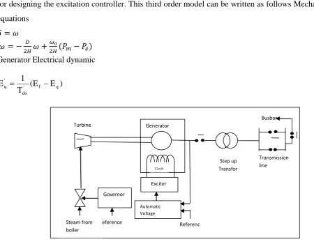
state operation, and also reduces the voltage oscillations during transient periods, affecting the

overall system stability. Fig.1 illustrates the AVR model used in the program developed.

Fig.1 AVR Model

The Synchronous Generator Model (Plant)

Fig.2 below shows a functional block diagram of synchronous generator connected to bus

bar through a step-up transformer. It also indicates the terminal voltage/reactive power control loop

using automatic voltage regulator (AVR) and the load frequency and real power control (LFC) loop

using the governor. During faulted condition, a single machine infinite bus power system shown in

Fig. 4 is used.

Fig.3 above is used to study the oscillation of the synchronous generator terminal voltage

under faulted condition. It has been shown that the dynamic response of (SG) in a practical power

system when a fault occurs is very complicated including much nonlinearity such as the magnetic

saturation. However, the classical third order dynamic generator model has been commonly used

for designing the excitation controller. This third order model can be written as follows Mechanical

equations

𝛿= 𝜔

𝜔= −_2𝐻𝐷 𝜔+𝜔0

2𝐻(𝑃𝑚− 𝑃𝑒) (1)

Generator Electrical dynamic

) E E ( T 1

E ' f q

do '

q = −

Fig. 2:Power system network showing AVR and LFC loops

Fig.3A single machine infinite bus power system

𝑋𝑆 𝑋𝑆 Generator Transformer G Fault 𝑉𝐿

Electrical equations

𝐸𝑞 =_𝑥𝑥𝑑𝑠

𝑑𝑜′ 𝐸 −

𝑥_{𝑑−𝑥𝑑′}

𝑥_𝑑𝑜′ 𝑉𝑠𝐶𝑜𝑠𝛿 (2)

𝑃𝑒 =_𝑥𝑉_𝑑𝑠𝑠 𝐸𝑞𝑆𝑖𝑛𝛿 (3)

𝐼𝑞 =_𝑥𝑉_𝑑𝑠𝑠 𝑆𝑖𝑛𝛿 = _𝑥𝑑𝑠𝑃𝑒_𝐼𝑓 (4)

𝑄𝑒 =_𝑥𝑉𝑠

𝑑𝑠𝐸𝑞𝐶𝑜𝑠𝛿 −

𝑉𝑠2

𝑥𝑑𝑠 (5)

R𝐸𝑞 =𝑥𝑎𝑑𝐼𝑓 R(6)

𝐸𝑓 =𝑘𝑐𝑈𝑓 (7)

𝑉𝑡= _𝑥1 𝑑𝑠�𝑥𝑠

2_𝐸

𝑞2+𝑉𝑠2𝑥𝑑2+ 2𝑥𝑐𝑥𝑑𝑥𝑑𝑠𝑃𝑒𝐶𝑜𝑠𝛿� 1_�2

𝑥𝑑𝑠 =𝑥𝑑+𝑥𝑇+𝑥𝐿 𝑥𝑑𝑠′ =𝑥𝑑′ +𝑥𝑇+𝑥𝐿 (8)

𝑋𝑠 =𝑋𝑇+𝑋𝐿 (9)

The definition of the parameters are given below

δ (t) power angle of the generator (in radian)

ω(t) relative speed (in rad/s)

PRmRmechanical input power (in p.u.)

PReRactive power delivered to bus (in p.u.)

ERq′R transient EMF in the quadrature axis (in p.u.)

VRt Rterminal voltage of the generator (in p.u.)

By linearizing the above equations about the operating point, we have the state equation as 𝑥̇= 𝐴𝑥+𝐵𝑢

A Fuzzy Model Reference Learning Controller for Synchronous Generator Terminal Voltage Control

y = cx (10) Where state variables x is defined as

x = (Δδ , Δω, ΔEq′) (11) and the control input and the output.

The matrices A, B, and C are given by

𝐴=�

0 1 0

𝑤𝑜𝑣𝑠

2𝐻𝑥′𝑑𝑠𝐼𝑞𝑐𝑜𝑠𝛿

−𝐷 2𝐻

−𝑤𝑜𝑣𝑠

2𝐻𝑥′𝑑𝑠 −𝐸′𝑞−𝑥′𝑑I𝑑

𝑉𝑡 �

−𝑥′𝑑

𝑥′𝑑𝑠� 𝑣𝑠𝑠𝑖𝑛𝛿 0

𝐵=�

0 0 𝑘𝑐 𝑇_𝑑𝑜′

� 𝐶=�𝐸𝑞−𝑥′𝑑𝐼𝑑

𝑉𝑡 �

−𝑥𝑑′

𝑥_𝑑𝑠′ � 𝑉𝑠sin𝛿+ 𝑥′𝑑𝐼𝑞

𝑉𝑡 �

𝑉𝑠

𝑥_𝑑𝑠′ �cos𝛿 0

𝐸𝑞′−𝑥𝑑′𝐼𝑑

𝑉𝑡 �1−

𝑥𝑑′

𝑥_𝑑𝑠′ ��

4. Interval Type-2 Fuzzy Logic Controllers

The interval type-2 FLC uses interval type-2 fuzzy sets (such as those shown in Fig. 4(a) to

represent the inputs and/or outputs of the FLC. In the interval type-2 fuzzy sets all the third

dimension values equal to one. The use of interval type-2 FLC helps to simplify the computation (as

opposed to the general type-2 FLC which is computationally intensive) which will enable the design

of an interval type-2 fuzzy logic controller (IT2FLC)that operates in real time. The structure of an

interval type-2 FLC is depicted in Fig.4(b), it consists of a Fuzzifier, Inference Engine, Rule Base,

Type-Reducer and a Defuzzifier.

Fig.4 (a) An interval type-2 fuzzy set. (b) Structure of the interval type-2 FLC.

The interval type-2 FLC works as follows: the crisp inputs from the input sensors are first

fuzzified into input type-2 fuzzy sets; singleton fuzzification is usually used in interval type-2 FLC

applications due to its simplicity and suitability for embedded processors and real time applications.

The input type-2 fuzzy sets then activate the inference engine and the rule base to produce output

type-2 fuzzy sets. The type-2 FLC rules will remain the same as in a type-1 FLC but the antecedents

and/or the consequents will be represented by interval type-2 fuzzy sets. The inference engine

combines the fired rules and gives a mapping from input type-2 fuzzy sets to output type-2 fuzzy

sets. The type-2 fuzzy outputs of the inference engine are then processed by the type-reducer which

combines the output sets and performs a centroid calculation which leads to type-1 fuzzy sets called

the type-reduced sets. There are different types of type-reduction methods. In this paper we will be

using the Center of Sets type-reduction as it has reasonable computational complexity that lies

between the computationally expensive centroid type-reduction and the simple height and modified

height type-reductions which have problems when only one rule fires. After the type-reduction

process, the type-reduced sets are defuzzified (by taking the average of the type-reduced set) to

obtain crisp outputs that are sent to the actuators.

The synchronous generator which represents the plant has an input u(kT) from the fuzzy

controller and terminal voltage output y(kT). The input to the fuzzy controller is the error e

(

)

r

(

)

(

)

𝑇 where r

(

)

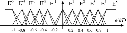
Membership functions for Interval type-2 Fuzzy logic controller inputs e

(

)

Fig.5 a,b & c.

A fuzzy rules were employed as indicated below in table 1 with triangular membership

functions.

Table 1:Decision table

In the table above, NV, NL, NB, NM, NS, ZR, PS, PM, PB, Pl, PV stands for negative very

large, negative large, negative big, negative medium, negative small, zero, positive small, positive

medium, positive big, positive large, and positive very large

E-5 E-4 E-3 E-2 E-1 E1 E2 E3 E4 E5

0.2 0.4 0.6 0.8 1 -1 -0.8 -0.6 -0.4 -0.2

e(kT)

Fig. 5a: Membership functions for input error e(kT)

C-5 C-4 C-3 C-2 C-1 C1 C2 C3 C4 C5

0.2 0.4 0.6 0.8 1 -1 -0.8 -0.6 -0.4 -0.2

c(kT)

Fig. 5b: Membership functions for input change in error c(kT)

5. The GA based System

The GA chromosome includes the interval type-2 MFs parameters for both the inputs and

outputs of the interval type-2 FLC. We have used the interval type-2 fuzzy set which is described by

a triangular MF. The GA based system uses real value encoding to encode each gene in the

chromosome. Each GA population consists of 30 chromosomes. The GA uses an elitist selection

strategy. The GA based system procedure can be summarized as follows:

Step 1: 30 chromosomes are generated randomly while taking into account the grammatical

correctness of the chromosome). The “Chromosome Counter” is set to 1– the first chromosome.

The “Generation Counter” is set to 1– the first generation.

Step 2: Interval Type-2 FLC is constructed using the chromosome “Chromosome Counter” and is

executed on the transient stability control for 400 iterations to provide a fitness for the

chromosome. After a controller has been executed for 400 iterations, a fixed controller takes

over control and returns to a correct position.

Step 3: If “Chromosome Counter” < 30, increment “Chromosome Counter” by 1 and go to Step 2,

otherwise proceed to Step 4.

Step 4: The best individual-so-far chromosome is preserved separately.

Step 5: If “Generation Counter” = 1 then store current population, copy it to a new population P and

proceed to Step 6. Else, select 30 best chromosomes from population “Generation Counter”

and population “Generation Counter”-1 and create a new population P.

Step 6: Use roulette wheel selection on population P to populate the breeding pool.

Step 7: Crossover is applied to chromosomes in the breeding pool and “chromosome consistency”

is checked. (*)

Step 8: “Generation Counter” is incremented. If “Generation Counter” < the number of maximum

generations or if the desired performance is not achieved, reset “Chromosome Counter” to 1

and go to Step 2, else go to Step 9.

Step 9: Chromosome with best fitness is kept and solution has been achieved; END.

(*)The crossover operator employed computes the arithmetic average between two genes. It

is used with a probability of 100% to force the GA to explore the solution space in between the

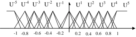
previously discovered, parental solutions. With chromosome consistency we refer to the correctness U-5 U-4 U-3 U-2 U-1 U1 U2 U3 U4 U5

0.2 0.4 0.6 0.8 1 -1 -0.8 -0.6 -0.4 -0.2

Fig. 5c: Membership functions for output u(kT)

of the chromosome’s genes in relation to their function in the IT2FLC. While the chromosome’s

genes are rearranged to achieve this, we eliminate a chromosome from the population if it violates

these criteria. The violating chromosome is replaced by a new, randomized but consistent

chromosome thus introducing new genetic material into the population at the same time.

In these experiments, the interval type-2 FLC has two sonar sensors as inputs which are

represented by two Triangular interval type-2 MFs (error e(kT) & change in error c(kT)). Therefore

each input interval type-2 MF is represented by three parameters (one singleton apex and two

extremities). Thus, 12 genes are used to represent the interval type-2 FLC inputs (The IT2FLC has 2

input sensors, each represented by two interval type-2 MFs and each MF is represented by 3

parameters). The interval type-2 FLC has 1 output u(kT). The IT2FLC output is represented by a

triangular interval type-2 MFs. Hence as shown in Fig. 6(a), the GA chromosome for this type-2

FLC comprises 12(inputs) + 4(outputs) = 16 genes.

Fig.6. (a) Chromosome Structure, (b) Progress of best individual.

Through various experiments, it was found that the GA based system evolves to good

interval type-2 MFs after about only 14 generations. An example of the evolutionary progress is

shown in Fig. 6(b) which shows the performance of the best individual found so far against the

number of generations.

Genetic algorithm-based parameter Learning

GAs is optimization stochastic techniquemimicking the natural selection, whichconsists of

three operations, namely,reproduction, crossover, and mutation.The most general considerations

about GA canbe stated as follows:

i) The searching procedure of the GA starts from multiple initial states simultaneously and proceeds

in all of the parameter subspaces simultaneously.

ii) GA requires almost no prior knowledge of the concerned system, which enables it to deal with

the completely unknown systems that other optimization methods may fail.

iii) GA cannot evaluate the performance of a system properly at one step. For this reason, it can

generally not be used as an on-line optimization strategy and is more suitable for fuzzy

modeling.

In practice, training data can be obtained by experimentation or by the establishment of an

ideal model. Fig.7 shows the training process for interval type-2 fuzzy controller (IT2FLC)

involved in the self-tuning system.

The following two closed-loop performance indices have been examined; the Integrated

Absolute Error (IAE) and the integrated time multiplied by the absolute error (ITAE). They are

defined as follows:

𝐽𝐼𝐴𝐸=IAE=∫₀𝑇|𝑒(𝑡)|𝑑𝑡=∑𝑘=0𝑀 |𝑟(𝑘)− 𝑦(𝑘)|Δt

𝐽𝐼𝐴𝑇𝐸=IATE=∫ 𝑡₀𝑇 |𝑒(𝑡)|𝑑𝑡=∑𝑀𝑘=0𝑘|𝑟(𝑘)− 𝑦(𝑘)|Δ𝑡2

Where e=𝑟(𝑘𝑇)− 𝑦(𝑘𝑇) is the closed loop error, r(kT) is the reference input, y(kT) terminal

voltage output and Δt is the time step. M is the number of training samples. Because GA endeavors

to maximize the fitness function, the fitness function of each gene is calculated as follows:

F= 1

1+𝐽 (12)

Where J is the performance index and 1 is introduced at the denominator to prevent the

fitness function from becoming infinitely large.

Coding of the parameters to be adjusted can be stated as follows:

c RN1R,c RN 2R,... σRN1R,σ RN 2R… uR11R,uR12R,… (13)

If identical input membership is chosen, the total number of parameters is reduced to 121

i.e. parameters of the input membership functions c RN1R, σ RN1R,c RZ1R, σRZ1Rc RP1R, σRP1R for e(kT), c RN2R, σ RN2R,c RZ2R, σRZ2R,c RP2R, σRP2R for c(kT) ,

Where a certain number of each binary bits stand for each element.

Fig.7 Genetic learning of the data-base of each module.

6. Simulation Results

The graphs shown in the subsection below will provide the comparative performance results

between the conventional control and the evolutionary interval type-2 fuzzy one. Two different

situations were analyzed; the first analysis is a one synchronous machine excitation control done

with the Matlab Software, the second one was done using a transient stability program called

"Transufu" applied to 18 bus bar IEEE system.

Interval type-2 Fuzzy Logic Controller Results applied to a One Synchronous Machine System

The block diagram shown in Fig.8 shows a synchronous machine for which output the

voltage is controlled by an AVR applied to its excitation system, in the MATLAB simulation. All

data were taken from reference.

Fig.8 Interval type-2 Fuzzy logic Controller basic configuration

Fuzzy Output constrain Knowledge

Base Rule

Data Base

Inference Relations

Decision centre

Inference Machine

Defuzzificati Fuzzification

Fuzzy input constraints

Output Inputs

Next step is to replace the AVR device by an interval type-2 fuzzy logic controller in order

to check its efficiency in the synchronous machine excitation voltage control. The rule-base used by

IT2FLC controller to simulate an AVR in the MATLAB program is shown in Table 2. The fuzzy

controller ran with the input and output normalized universe [-1,1]. The seven linguistic variables

used were generator voltage error e(kT) and generator voltage error variation c(kT), which are: LN -

large negative, MN - medium negative, SN - small negative, Z – zero, SP - small positive, MP -

medium positive, LP - large positive

Table 2: The output rule base used by IT2FLC in MATLAB program simulation.

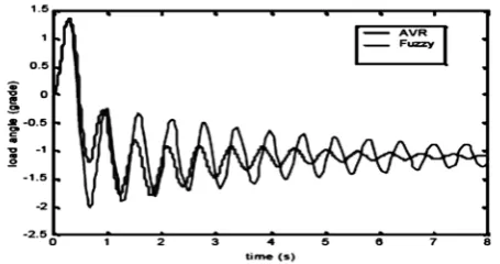
Fig.9,10 & 11 show the terminal voltage, load angle and electrical torque of a synchronous machine

connected to an infinite bus bar by a transmission line.

Fig.9 One machine analysis (terminal voltage Vt.) using IT2FLC

Fig.10 One machine analysis (load angle) using IT2FLC

Fig.11 One machine analysis (electrical torque) using IT2FLC

Following test cases are simulated below for Conventional Automatic Voltage Regulator (CAVR),

A step input is applied to a normal CAVR with amplifier transfer function given by

𝐾𝐴

1+𝜏𝐴𝑆 (14) KA =10, τG = 0.1, KE =1, 𝜏E = 0.4

KG =1,𝜏G =1, KR =1, 𝜏R = 0.05 Below is the step response in Fig.12.

A stabilizer is connected between the exciter output and the input summer with a step input

signal. The parameters above remained the same but the stabilizer has transfer function given by 𝑠

0.04𝑠+ 1

Fig.12Terminal voltage step response for CAVR The terminal voltage step response of CAVR with stabilizer is shown in Fig.13.

t, sec

1.8 1.6 1.4 1.2 1 0.8 0.6 0.4 0.2

18 16 14 12 10 8 6 4 2 0

Fig.13 Terminal voltage step response of CAVR with stabilizer

4. IT2FLC-AVR is used and the response for a step input is shown in Fig. 14 (a) and (b). A three

phase fault is applied to the line and cleared after two seconds. Fig15 (a) and (b) shows the

Response

Fig.14 Step response of IT2FLC-AVR

Fig.15Step response of IT2FLC -AVR to a three phase fault.

7. Conclusion

This paper reviewed the various techniques employed in synchronous generator terminal

voltage control. Such techniques are the CAVR, MV, GMV, PP and ordinary fuzzy controller. It

identified some of the limitation of each of them, such as the steady state error presented by

ordinary fuzzy controller. The application of IT2FLC controller is the main focus of this paper. The

simulation results for disturbed terminal voltage values and transmission lines faults shows a very

sharp reduction in settling time, over shoot, rise time and zero steady state error. It could be

observed in study using MATLAB simulation, an excellent response of the IT2FLC controller and

with no oscillation, while the AVR response presented a ripple in both studies and some oscillations

before reaching the steady state operation point. It is shown that an excellent performance of the

IT2FLC control over the conventional AVR one for the excitation control of synchronous machines

could be achieved. It has been shown that the genetically evolved interval type-2 FLCs can lead to

superior performance in comparison to interval type-1 FLCs and the manually designed interval

type-2 FLCs. The results indicate that the genetic evolution of interval type-2 MFs can provide

valid and high-performance interval type-2 FLCs without relying on any a priori knowledge such as

logged data or a previously existing model, making it suitable for control problems where no such a

priori data is available such as in transient stability control in power system. This work will be a

step towards overcoming the problem of manually specifying pseudo-optimal MFs for interval

type-2 FLCs, which to date is one of the main obstacles when designing interval type-type-2 FLCs.

References

1. Anderson P.M. and Fouad A.A.; (1977) “Power System Control and Stability”- The Iowa

State University Press, Ames, Iowa, USA,

2. Mamdani E.H. and Assilian S.; (1975) “An experiment in linguistic synthesis with a fuzzy

logic controller”, Int. J. Man Mach. Studies, Vol. 7, No. 1, pp. 1-13.

3. Alba E., Cotta C. and Troya J. M. (1999) “Evolutionary Design of Fuzzy Logic Controllers

Using Strongly-Typed GP”; Mathware & Soft Computing, Vol. 6, Issue 1, pp. 109-124.

4. Cordon O., Herrera F., Hoffmann F, and Magdalena L (2001) “Genetic Fuzzy System:

Evolutionary Tuning and Learning of Fuzzy Knowledge Bases”; Singapore: World

Scientific.

5. Figueroa J., Posada J., Soriano J., Melgarejo M and Roj S. (2005) “A type-2 fuzzy logic

controller for tracking mobile objects in the context of robotic soccer games”; Proceeding

of the 2005 IEEE International Conference on Fuzzy Systems, pp. 359-364, 25-25 May

2005, Reno, USA.

6. Hagras H. (2004) "A Hierarchical type-2 Fuzzy Logic Control Architecture for

Autonomous Mobile Robots”; IEEE Transactions on Fuzzy Systems, Vol. 12 No. 4, pp.

524-539.

7. Hagras H., Colley M. and Callaghan V. (2004) “Learning and Adaptation of an Intelligent

Mobile Robot Navigator Operating in Unstructured Environment Based on a Novel Online

Fuzzy-Genetic System”; Journal of Fuzzy Sets and Systems, Vol. 141, No. 1, pp. 107-160.

8. Hoffmann F. and Pfister G.; (1997) “ Evolutionary Design of a fuzzy knowledge base for a

mobile robot”; International Journal of Approximate Reasoning, Vol. 17, No. 4,

pp.447-469.

9. Liang Q. and Mendel J.; (2000) “Interval type-2 Fuzzy Logic Systems: Theory and Design;

IEEE Transactions on Fuzzy Systems, Vol. 8, No.5, pp. 535 - 550.

10.Lynch C., Hagras H. and Callaghan V.; (July 2006) “Using Uncertainty Bounds in the

Design of an Embedded Real-Time type-2 Neuro-Fuzzy Speed Controller for Marine Diesel

Engines”; Proceedings of the 2006 IEEE International Conference of Fuzzy Systems, pp.

1446 – 1453, Vancouver, Canada.

11.Lynch C., Hagras H. and Callaghan V.; (July 2006) “ Embedded Interval type-2

Neuro-Fuzzy Speed Controller for Marine Diesel Engines”; Proceedings of the 2006 Information

Processing and Management of Uncertainty in Knowledge-based Systems conference, pp.

1340-1347, Paris, France.

12.Mendel J. (2001) “Uncertain Rule-Based Fuzzy Logic Systems”; Prentice Hall.

13.Mendel J. and John R.; (April 2002) “Type-2 Fuzzy Sets Made Simple”; IEEE Transactions

on Fuzzy Systems, Vol. 10, Issue 2, pp.117-127, April 2002.

14.Mendel J. and Wu H.; (2002) “Uncertainty versus choice in rule-based fuzzy logic

systems”; Proceedings of IEEE International Conference of Fuzzy Systems, pp.1336-1341,

12 May 2002-17 May 2002, Honolulu.

15.Wan T.W. and Kamal D.H. (July 2006) “On-line Learning Rules For type-2 Fuzzy

Controller”; Proceedings of the 2006 IEEE International Conference of Fuzzy Systems, pp.

513-520,Vancouver, Canada.

16.Wu H. and Mendel J. (October 2002) “Uncertainty Bounds and Their Use in the Design of

Interval type-2 Fuzzy Logic Systems”; IEEE Transactions on Fuzzy Systems, Vol. 10, No.

5, pp.622-639.

17.Wu .D and Tan W.W; 2004 “A type-2 Fuzzy logic Controller for the Liquid-level Process”;

Fuzz-IEEE 2004, IEEE International Conference on Fuzzy Systems, Budapest; pp. 953 –

958, Vol.20T , 0T25-29 July 2004

18.Wu D. and Tan W.W.; (May 2005) “Type-2 FLS modeling capability analysis”;

Proceedings of the 2005 IEEE International Conference on Fuzzy Systems, pp. 242-247;

Reno, USA.

19.Wen J.Y, Cheng S.G, Malik.O.P; (August 1998) “A synchronous generator fuzzy excitation

controller optimally designed with a genetic algorithm”, IEEE Transactions on power

systems Vol.13, No.3, pp. 884–889.

20.Ruhua You., Hassan J., Eghbali M., Hashem N., (February 2003) “An online Adaptive

Neuro- Fuzzy power system stabilizer for multi-machine systems”, IEEE Transactions on

power system. Vol. 18, No. 1, pp 128–135.

21.Guo Yi., David J. H. and Youyi W.; (Nov 2001) “Global Transient stability and voltage

regulation for power systems”, IEEE Transactions on power systems, Vol. 16, No. 4, pp.

678-688.

---