Bayesian Policy Gradient and Actor-Critic Algorithms

(1)

Bayesian Policy Gradient and Actor-Critic Algorithms

Mohammad Ghavamzadeh∗ [email protected]

Adobe Research & INRIA

Yaakov Engel [email protected]

Rafael Advanced Defence System, Israel

Michal Valko [email protected]

INRIA Lille — SequeL team, France

Editor:Jan Peters

Abstract

Policy gradient methods are reinforcement learning algorithms that adapt a param-eterized policy by following a performance gradient estimate. Many conventional policy gradient methods use Monte-Carlo techniques to estimate this gradient. The policy is improved by adjusting the parameters in the direction of the gradient estimate. Since Monte-Carlo methods tend to have high variance, a large number of samples is required to attain accurate estimates, resulting in slow convergence. In this paper, we first pro-pose a Bayesian framework for policy gradient, based on modeling the policy gradient as a Gaussian process. This reduces the number of samples needed to obtain accurate gra-dient estimates. Moreover, estimates of the natural gragra-dient as well as a measure of the uncertainty in the gradient estimates, namely, the gradient covariance, are provided at little extra cost. Since the proposed Bayesian framework considers system trajectories as its basic observable unit, it does not require the dynamics within trajectories to be of any particular form, and thus, can be easily extended to partially observable problems. On the downside, it cannot take advantage of the Markov property when the system is Markovian.

To address this issue, we proceed to supplement our Bayesian policy gradient framework with a new actor-critic learning model in which a Bayesian class of non-parametric critics, based on Gaussian process temporal difference learning, is used. Such critics model the action-value function as a Gaussian process, allowing Bayes’ rule to be used in computing the posterior distribution over action-value functions, conditioned on the observed data. Appropriate choices of the policy parameterization and of the prior covariance (kernel) between action-values allow us to obtain closed-form expressions for the posterior distri-bution of the gradient of the expected return with respect to the policy parameters. We perform detailed experimental comparisons of the proposed Bayesian policy gradient and actor-critic algorithms with classic Monte-Carlo based policy gradient methods, as well as with each other, on a number of reinforcement learning problems.

Keywords: reinforcement learning, policy gradient methods, actor-critic algorithms, Bayesian inference, Gaussian processes

(2)

1. Introduction

Policy gradient (PG) methods1 are reinforcement learning (RL) algorithms that maintain a parameterized action-selection policy and update the policy parameters by moving them in the direction of an estimate of the gradient of a performance measure. Early examples of PG algorithms are the class of REINFORCE algorithms (Williams, 1992),2 which are suitable for solving problems in which the goal is to optimize the average reward. Subse-quent work (e.g., Kimura et al., 1995, Marbach, 1998, Baxter and Bartlett, 2001) extended these algorithms to the cases of infinite-horizon Markov decision processes (MDPs) and partially observable MDPs (POMDPs), while also providing much needed theoretical anal-ysis.3 _{However, both the theoretical results and empirical evaluations have highlighted a}

major shortcoming of these algorithms, namely, the high variance of the gradient estimates. This problem may be traced to the fact that in most interesting cases, the time-average of the observed rewards is a high-variance (although unbiased) estimator of the true average reward, resulting in the sample-inefficiency of these algorithms.

One solution proposed for this problem was to use an artificial discount factorin these algorithms (Marbach, 1998, Baxter and Bartlett, 2001), however, this creates another prob-lem by introducing bias into the gradient estimates. Another solution, which does not involve biasing the gradient estimate, is to subtract areinforcement baselinefrom the aver-age reward estimate in the updates of PG algorithms (e.g., Williams, 1992, Marbach, 1998, Sutton et al., 2000). In Williams (1992) an average reward baseline was used, and in Sut-ton et al. (2000) it was conjectured that an approximate value function would be a good choice for a state-dependent baseline. However, it was shown in Weaver and Tao (2001) and Greensmith et al. (2004), perhaps surprisingly, that the mean reward is in generalnot

the optimal constant baseline, and that the true value function is generallynotthe optimal state-dependent baseline.

A different approach for speeding-up PG algorithms was proposed by Kakade (2002) and refined and extended by Bagnell and Schneider (2003) and Peters et al. (2003). The idea is to replace the policy gradient estimate with an estimate of the so-called natural policy gradient. This is motivated by the requirement that the policy updates should be invariant to bijective transformations of the parametrization. Put more simply, a change in the way the policy is parametrized should not influence the result of the policy update. In terms of the policy update rule, the move to natural-gradient amounts to linearly transforming the gradient using the inverse Fisher information matrix of the policy. In empirical evaluations, natural PG has been shown to significantly outperform conventional PG (e.g., Kakade 2002, Bagnell and Schneider 2003, Peters et al. 2003, Peters and Schaal 2008).

1. The term has been coined in Sutton et al. (2000), but here we use it more liberally to refer to a whole class of reinforcement learning algorithms.

2. Note that policy gradient methods have been studied in the control community (see e.g., Dyer and McReynolds 1970, Jacobson and Mayne 1970, Hasdorff 1976) before REINFORCE. However, unlike REINFORCE that is model-free, they were all based on the exact model of the system (model-based). 3. It is important to note that the pioneering work of Gullapali and colleagues in the early 1990s (Gullapalli,

(3)

Another approach for reducing the variance of policy gradient estimates, and as a result making the search in the policy-space more efficient and reliable, is to use an explicit representation for the value function of the policy. This class of PG algorithms are called actor-critic algorithms. Actor-critic (AC) algorithms comprise a family of RL methods that maintain two distinct algorithmic components: An actor, whose role is to maintain and update an action-selection policy; and a critic, whose role is to estimate the value function associated with the actor’s policy. Thus, the critic addresses the problem of prediction, whereas the actor is concerned withcontrol. Actor-critic methods were among the earliest to be investigated in RL (Barto et al., 1983, Sutton, 1984). They were largely supplanted in the 1990’s by methods, such as SARSA (Rummery and Niranjan, 1994), that estimate action-value functions and use them directly to select actions without maintaining an explicit representation of the policy. This approach was appealing because of its simplicity, but when combined with function approximation was found to be unreliable, often failing to converge. These problems led to renewed interest in PG methods.

Actor-critic algorithms (e.g., Sutton et al. 2000, Konda and Tsitsiklis 2000, Peters et al. 2005, Bhatnagar et al. 2007) borrow elements from these two families of RL algorithms. Like value-function based methods, a critic maintains a value function estimate, while an actor maintains a separately parameterized stochastic action-selection policy, as in policy based methods. While the role of the actor is to select actions, the role of the critic is to evaluate the performance of the actor. This evaluation is used to provide the actor with a feedback signal that allows it to improve its performance. The actor typically updates its policy along an estimate of the gradient (or natural gradient) of some measure of performance with respect to the policy parameters. When the representations used for the actor and the critic are compatible, in the sense explained in Sutton et al. (2000) and Konda and Tsitsiklis (2000), the resulting AC algorithm is simple, elegant, and provably convergent (under appropriate conditions) to a local maximum of the performance measure used by the critic, plus a measure of the temporal difference (TD) error inherent in the function approximation scheme (Konda and Tsitsiklis, 2000, Bhatnagar et al., 2009).

Existing AC algorithms are based on parametric critics that are updated to optimize frequentist fitness criteria. By “frequentist” we mean algorithms that return a point esti-mate of the value function, rather than a complete posterior distribution computed using Bayes’ rule. A Bayesian class of critics based on Gaussian processes (GPs) has been pro-posed by Engel et al. (2003, 2005), called Gaussian process temporal difference (GPTD). By their Bayesian nature, these algorithms return a full posterior distribution over value functions. Moreover, while these algorithms may be used to learn a parametric represen-tation for the posterior, they are generally capable of searching for value functions in an infinite-dimensional Hilbert space of functions, resulting in a non-parametric posterior.

Both conventional and natural policy gradient and actor-critic methods rely on Monte-Carlo (MC) techniques in estimating the gradient of the performance measure. MC es-timation is a frequentist procedure, and as such violates the likelihood principle (Berger and Wolpert, 1984).4 _{Moreover, although MC estimates are unbiased, they tend to suffer}

from high variance, or alternatively, require excessive sample sizes (see O’Hagan, 1987 for

(4)

a discussion). In the case of policy gradient estimation this is exacerbated by the fact that consistent policy improvement requires multiple gradient estimation steps.

In O’Hagan (1991) a Bayesian alternative to MC estimation is proposed.5 The idea is to model integrals of the formR

f(x)g(x)dxas GPs. This is done by treating the first term f in the integrand as a random function, the randomness of which reflects our subjective uncertainty concerning its true identity. This allows us to incorporate our prior knowledge of f into its prior distribution. Observing (possibly noisy) samples of f at a set of points

{x1, . . . , xM} allows us to employ Bayes’ rule to compute a posterior distribution of f

conditioned on these samples. This, in turn, induces a posterior distribution over the value of the integral.

In this paper, we first propose a Bayesian framework for policy gradient estimation by modeling the gradient as a GP. Our Bayesian policy gradient (BPG) algorithms use GPs to define a prior distribution over the gradient of the expected return, and compute its posterior conditioned on the observed data. This reduces the number of samples needed to obtain accurate gradient estimates. Moreover, estimates of the natural gradient as well as a measure of the uncertainty in the gradient estimates, namely the gradient covariance, are provided at little extra cost. Additional gains may be attained by learning a transition model of the environment, allowing knowledge transfer between policies. Since our BPG models and algorithms consider complete system trajectories as their basic observable unit, they do not require the dynamics within each trajectory to be of any special form. In particular, it is not necessary for the dynamics to have the Markov property, allowing the resulting algorithms to handle partially observable MDPs, Markov games, and other non-Markovian systems. On the downside, BPG algorithms cannot take advantage of the Markov property when this property is satisfied. To address this issue, we supplement our BPG framework with actor-critic methods and propose an AC algorithm that incorporates GPTD as its critic. However, rather than merely plugging-in our critic into an existing AC algorithm, we show how the posterior moments returned by the GPTD critic allow us to obtain closed-form expressions for the posterior moments of the policy gradient. This is made possible by utilizing the Fisher kernel (Shawe-Taylor and Cristianini, 2004) as our prior covariance kernel for the GPTD state-action advantage values. Unlike the BPG methods, the Bayesian actor-critic (BAC) algorithm takes advantage of the Markov property of the system trajectories and uses individual state-action-reward transitions as its basic observable unit. This helps reduce variance in the gradient estimates, resulting in steeper learning curves when compared to BPG and the classic MC approach.

It is important to note that a short version of the two main parts of this paper,Bayesian policy gradient and Bayesian actor-critic, appeared in Ghavamzadeh and Engel (2006) and Ghavamzadeh and Engel (2007), respectively. This paper extends these conference papers in the following ways:

• We have included a discussion on using Bayesian Quadrature (BQ) for estimating vector-valued integrals to the paper. This is totally relevant to this work because the gradient of a policy (the quantity that we are interested in estimating using BQ) is a vector-valued integral when the size of the policy parameter vector is more than 1, which is usually the case. This also helps to better see the difference between

(5)

the two models we propose for BPG. In Model 1, we place a vector-valued Gaussian process (GP) over a component of the gradient integrant, while in Model 2, we put a scalar-valued GP over a different component of the gradient integrant.

• We describe the BPG and BAC algorithms in more details and show the details of using online sparsification in these algorithms. Moreover, we show how BPG can be extended to partially observable Markov decision processes (POMDPs) along the same lines that the standard PG algorithms can be used in such problems.

• In comparison to Ghavamzadeh and Engel (2006), we report more details of the ex-periments and more experimental results, especially in using the posterior variance (covariance) of the gradient to select the step size for updating the policy parameters.

• We include all the proofs in this paper (almost none was reported in the two conference papers), in particular, the proofs of Propositions 3, 4, 5, and 6. These proofs are important and the proof techniques are novel and definitely useful for the community. The importance of these proofs come from the fact that they show how with the right choice of GP prior (the one that uses the family of Fisher information kernels), we are able to use BQ and have a Bayesian estimate of the gradient integral, while initially everything indicates that BQ cannot be used for the estimation of this integral.

• We apply the BAC algorithm to two new domains: “Mountain Car”, a 2-dimensional continuous state and 1-dimensional discrete action problem, and “Ship Steering”, a 4-dimensional continuous state and 1-dimensional continuous action problem.

2. Reinforcement Learning, Policy Gradient, and Actor-Critic Methods

Reinforcement learning (RL) (Bertsekas and Tsitsiklis, 1996, Sutton and Barto, 1998) is term describing a class of learning problems in which an agent (or controller) interacts with a dynamic, stochastic, and incompletely known environment (or plant), with the goal of finding an action-selection strategy, or policy, to optimize some measure of its long-term performance. This interaction is conventionally modeled as a Markov decision process (MDP) (Puterman, 1994), or if the environmental state is not completely observable, as a partially observable MDP (POMDP) (Astrom, 1965, Smallwood and Sondik, 1973, Kael-bling et al., 1998). In this work we restrict our attention to the discrete-time MDP setting. LetP(X),P(A), andP(R) denote the set of probability distributions on (Borel) subsets

of the sets X, A, and R, respectively. A MDP is a tuple (X,A, q, P, P0) where X and A

are the state and action spaces; q(·|x, a) ∈ P(R) andP(·|x, a) ∈ P(X) are the probability

distributions over rewards and next states when action a is taken at state x (we assume thatq and P are stationary); andP0(·)∈ P(X) is the probability distribution according to

which the initial state is selected. We denote the random variable distributed according to q(·|x, a) as r(x, a) and its mean as ¯r(x, a).

(6)

Markov chain over state-action pairs zt= (xt, at) ∈ Z =X × A, with a transition proba-bility densityPµ(zt|zt−1) =P(xt|xt−1, at−1)µ(at|xt), and an initial state densityP0µ(z0) =

P0(x0)µ(a0|x0). We generically denote by ξ = (z0,z1, . . . ,zT) ∈ Ξ, T ∈ {0,1, . . . ,∞} a path generated by this Markov chain. Note that Ξ is the set of all possible trajectories that can be generated by the Markov chain induced by the current policy µ. The probability (density) of such a path is given by

Pr(ξ;µ) =P₀µ(z0)

T

Y

t=1

Pµ(zt|zt−1) =P0(x0)

T−1

Y

t=0

µ(at|xt)P(xt+1|xt, at). (1)

We denote by R(ξ) = PT−1

t=0 γtr(xt, at) the (possibly discounted, γ ∈ [0,1]) cumulative

returnof the pathξ. R(ξ) is a random variable both because the pathξ itself is a random variable, and because, even for a given path, each of the rewards sampled in it may be stochastic. The expected value of R(ξ) for a given path ξ is denoted by ¯R(ξ). Finally, we define theexpected return of policy µas

η(µ) =ER(ξ)=

Z

Ξ

¯

R(ξ) Pr(ξ;µ)dξ. (2)

The t-step state-action occupancy density of policyµis given by

P_tµ(zt) =

Z

Zt

dz0. . . dzt−1P₀µ(z0)

t

Y

i=1

Pµ(zi|zi−1).

It can be shown that under certain regularity conditions (Sutton et al., 2000), the expected return of policy µ may be written in terms of state-action pairs (rather than in terms of trajectories as in Equation 2) as

η(µ) =

Z

dzπµ(z)¯r(z), (3)

where πµ(z) = P∞

t=0γtP

µ

t (z) is a discounted weighting of state-action pairs encountered while following policyµ. Integratingaout ofπµ(z) =πµ(x, a) results in the corresponding discounted weighting of states encountered by following policy µ: νµ(x) = R_Adaπµ(x, a). Unlike νµ and πµ, (1−γ)νµ and (1−γ)πµ are distributions. They are analogous to the stationary distributions over states and state-action pairs of policy µ in the undiscounted setting, respectively, since as γ →1, they tend to these distributions, if they exist.

Our aim is to find a policyµ∗that maximizes the expected return, i.e.,µ∗= arg max_µη(µ). A policyµ is assessed according to the expected cumulative rewards associated with states x or state-action pairsz. For all statesx∈ X and actionsa∈ A, the action-value function and the value function of policyµare defined as

Qµ(z) =E

" _∞ X

t=0

γtr(zt)|z0 =z #

and Vµ(x) =

Z

A

daµ(a|x)Qµ(x, a).

(7)

by Equation 2 (or Equation 3), with respect to the policy parametersθ, from the observed system trajectories. We then improve the policy by adjusting the parameters in the direction of the gradient (e.g., Williams 1992, Marbach 1998, Baxter and Bartlett 2001). Since in this setting a policy µ is represented by its parameters θ, policy dependent functions such as η(µ), Pr ξ;µ), πµ(z), νµ(x), Vµ(x), and Qµ(z) may be written as η(θ), Pr(ξ;θ), π(z;θ), ν(x;θ),V(x;θ), andQ(z;θ), respectively. We assume

Assumption 1 (Differentiability) For any state-action pair (x, a) and any policy pa-rameter θ∈Θ, the policy µ(a|x;θ) is continuously differentiable in the parameters θ.

Thescore functionorlikelihood ratiomethod has become the most prominent technique for gradient estimation from simulation. It has been first proposed in the 1960’s (Aleksandrov et al., 1968, Rubinstein, 1969) for computing performance gradients in i.i.d. (independently and identically distributed) processes, and was then extended to regenerative processes in-cluding MDPs by Glynn (1986, 1990), Reiman and Weiss (1986, 1989), Glynn and L’Ecuyer (1995), and to episodic MDPs by Williams (1992). This method estimates the gradient of the expected return with respect to the policy parametersθ, defined by Equation 2, using the following equation:6

∇η(θ) =

Z

¯

R(ξ)∇Pr(ξ;θ)

Pr(ξ;θ) Pr(ξ;θ)dξ. (4)

In Equation 4, the quantity ∇_Pr(Pr(_ξ_;ξ_θ;θ₎) =∇log Pr(ξ;θ) is called the (Fisher) score function or likelihood ratio. Since the initial-state distributionP0 and the state-transition distribution

P are independent of the policy parameters θ, we may write the score function for a path ξ using Equation 1 as7

u(ξ;θ) =∇log Pr(ξ;θ) = ∇Pr(ξ;θ) Pr(ξ;θ) =

T−1

X

t=0

∇µ(at|xt;θ) µ(at|xt;θ) =

T−1

X

t=0

∇logµ(at|xt;θ). (5)

Previous work on policy gradient used classical MC to estimate the gradient in Equa-tion 4. These methods generate i.i.d. sample paths ξ1, . . . , ξM according to Pr(ξ;θ), and

estimate the gradient ∇η(θ) using the MC estimator

c

∇η(θ) = 1 M

M

X

i=1

R(ξi)∇log Pr(ξi;θ) = 1 M

M

X

i=1

R(ξi)

Ti−1

X

t=0

∇logµ(at,i|xt,i;θ). (6)

This is an unbiased estimate, and therefore, by the law of large numbers,∇cη(θ)→ ∇η(θ)

asM goes to infinity, with probability one.

The policy gradient theorem (Marbach, 1998, Proposition 1; Sutton et al., 2000, The-orem 1; Konda and Tsitsiklis, 2000, TheThe-orem 1) states that the gradient of the expected return, defined by Equation 3, for parameterized policies satisfying Assumption 1 is given by

∇η(θ) =

Z

dxda ν(x;θ)∇µ(a|x;θ)Q(x, a;θ). (7)

6. Throughout the paper, we use the notation∇to denote∇θ – the gradient w.r.t. the policy parameters.

(8)

Observe that ifb:X →_Ris an arbitrary function ofx (also called abaseline), then

Z

dxda ν(x;θ)∇µ(a|x;θ)b(x) =

Z

X

dx ν(x;θ)b(x)∇ Z

A

daµ(a|x;θ)=

Z

X

dx ν(x;θ)b(x)∇(1) = 0,

and thus, for any baselineb(x), the gradient of the expected return can be written as

∇η(θ) =

Z

dxda ν(x;θ)∇µ(a|x;θ) Q(x, a;θ) +b(x)=

Z

dzπ(z;θ)∇logµ(a|x;θ) Q(z;θ) +b(x).

(8)

The baseline may be chosen in such a way so as to minimize the variance of the gradient estimates (Greensmith et al., 2004).

Now consider the actor-critic (AC) framework in which the action-value function for a fixed policyµ,Qµ, is approximated by a learned function approximator. If the approxima-tion is sufficiently good, we may hope to use it in place of Qµ in Equations 7 and 8, and still point roughly in the direction of the true gradient. Sutton et al. (2000) and Konda and Tsitsiklis (2000) showed that if the approximation ˆQµ(·;w) with parameterwiscompatible, i.e., ∇_wQˆµ(x, a;w) =∇logµ(a|x;θ), and if it minimizes the mean squared error

Eµ(w) =

Z

dzπµ(z)Qµ(z)−Qˆµ(z;w)2 (9)

for parameter valuew∗, then we may replaceQµ with ˆQµ(·;w∗) in Equations 7 and 8. The second condition means that ˆQµ(·;w∗) is the projection ofQµonto the space{Qˆµ(·;w)|w∈

Rn}, with respect to a `2-norm weighted byπµ.

An approximation for the action-value function, in terms of a linear combination of basis functions, may be written as ˆQµ(z;w) =w>ψ(z). This approximation is compatible if the ψ’s are compatible with the policy, i.e., ψ(z;θ) =∇logµ(a|x;θ). Note that compatibility is well defined under Assumption 1. LetEµ₍_w_{) denote the mean squared error}

Eµ(w) =

Z

dzπµ(z)Qµ(z)−w>ψ(z)−b(x)2 (10)

of our compatible linear approximation w>ψ(z) and an arbitrary baseline b(x). Letw∗ = arg min_wEµ₍_w_{) denote the optimal parameter.} _{It can be shown that the value of} _w∗

does not depend on the baseline b(x). As a result, the mean squared-error problems of Equations 9 and 10 have the same solutions (see e.g., Bhatnagar et al. 2007, 2009). It can also be shown that if the parameter w is set to be equal to w∗, then the resulting mean squared errorEµ₍_w∗_{), now treated as a function of the baseline} _b₍_x_{), is further minimized}

by setting b(x) = Vµ(x) (Bhatnagar et al., 2007, 2009). In other words, the variance in the action-value function estimator is minimized if the baseline is chosen to be the value function itself.

A convenient and rather flexible choice for a space of policies that ensures compatibility between the policy and the action-value representation is a parametric exponential family

µ(a|x;θ) = 1 Zθ(x)

exp

θ>φ(x, a)

(9)

where Zθ(x) =

R

Adaexp θ

>_φ₍_{x, a}₎

is a normalizing factor, referred to as the partition function. It is easy to show thatψ(z) =φ(z)−Ea|x[φ(z)], whereEa|x[·] =

R

Adaµ(a|x;θ)[·],

and as a result, ˆQµ(z;w∗) =w∗> φ(z)−Ea|x[φ(z)]

+b(x) is a compatible action-value function for this family of policies. Note that E_a|x[ ˆQ(z;w∗)] = b(x), since Ea|x

φ(z)− Ea|x[φ(z)]

= 0. This means that if ˆQµ(z;w∗) approximates Qµ(z), then b(x) must ap-proximate the value functionVµ(x). The term ˆAµ(z;w∗) = ˆQµ(z;w∗)−b(x) =w∗> φ(z)− E_a|x[φ(z)]

approximates theadvantage functionAµ(z) =Qµ(z)−Vµ(x) (Baird, 1993).

3. Bayesian Quadrature

Bayesian quadrature (BQ) (O’Hagan, 1991) is, as its name suggests, a Bayesian method for evaluating an integral using samples of its integrand. We consider the problem of evaluating the integral

ρ=

Z

f(x)g(x)dx. (11)

If g(x) is a probability density function, i.e., g(x) = p(x), this becomes the problem of evaluating the expected value off(x). A well known frequentist approach to evaluating such expectations is the Monte-Carlo (MC) method. For MC estimation of such expectations, it is typically required that samples x1, x2, . . . , xM are drawn fromp(x).8 The integral in

Equation 11 is then estimated as

ˆ

ρM C = 1

M M

X

i=1

f(xi). (12)

It is easy to show that ˆρM C is an unbiased estimate of ρ, with variance that diminishes to zero asM → ∞. However, as O’Hagan (1987) points out, MC estimation is fundamentally unsound, as it violates the likelihood principle, and moreover, does not make full use of the data at hand. The alternative proposed in O’Hagan (1991) is based on the following reasoning: In the Bayesian approach,f(·) is random simply because it is unknown. We are therefore uncertain about the value off(x) until we actually evaluate it. In fact, even then, our uncertainty is not always completely removed, since measured samples off(x) may be corrupted by noise. Modeling f as a Gaussian process (GP) means that our uncertainty is completely accounted for by specifying a Normal prior distribution over functions. This prior distribution is specified by its mean and covariance, and is denoted byf(·)∼ N f¯(·), k(·,·). This is shorthand for the statement that f is a GP with prior mean and covariance

E

f(x)

= ¯f(x) and Cov

f(x), f(x0)

=k(x, x0), ∀x, x0 ∈ X, (13) respectively. The choice of kernel function k allows us to incorporate prior knowledge on the smoothness properties of the integrand into the estimation procedure. When we are provided with a set of samples DM =

xi, y(xi) M_i₌₁, where y(xi) is a (possibly noisy)

sample off(xi), we apply Bayes’ rule to condition the prior on these sampled values. If the measurement noise is normally distributed, the result is a Normal posterior distribution of

(10)

f|D_M. The expressions for the posterior mean and covariance are standard:

E

f(x)|D_M

= ¯f(x) +k(x)>C(y−f¯),

Covf(x), f(x0)|DM

=k(x, x0)−k(x)>Ck(x0). (14) Here and in the sequel, we make use of the definitions:

¯

f = f¯(x1), . . . ,f¯(xM)

>

, k(x) = k(x1, x), . . . , k(xM, x)

>

, y= y(x1), . . . , y(xM)

>

, [K]i,j=k(xi, xj), C = (K+Σ)−1,

where K is the kernel (or Gram) matrix, and [Σ]i,j is the measurement noise covariance between the ith and jth samples. It is typically assumed that the measurement noise is i.i.d., in which case Σ = σ2I, where σ2 is the noise variance and I is the (appropriately sized - hereM ×M) identity matrix.

Since integration is a linear operation, the posterior distribution of the integral in Equa-tion 11 is also Gaussian, and the posterior moments are given by (O’Hagan, 1991)

E[ρ|D_M] =

Z

E

f(x)|D_M

g(x)dx,

Var[ρ|DM] =

Z Z

Covf(x), f(x0)|DM

g(x)g(x0)dxdx0. (15)

Substituting Equation 14 into Equation 15, we obtain

E[ρ|D_M] =ρ0+b>C(y−f¯) and Var[ρ|DM] =b0−b>Cb,

where we made use of the definitions:

ρ0 =

Z

¯

f(x)g(x)dx , b=

Z

k(x)g(x)dx , b0= Z Z

k(x, x0)g(x)g(x0)dxdx0. (16) Note thatρ0 and b0 are the prior mean and variance of ρ, respectively.

Rasmussen and Ghahramani (2003) experimentally demonstrated how this approach, when applied to the evaluation of an expectation, can outperform MC estimation by orders of magnitude in terms of the mean-squared error.

In order to prevent the problem from “degenerating into infinite regress”, as phrased by O’Hagan (1991),9we should choose the functionsg,k, and ¯f so as to allow us to solve the integrals in Equation 16 analytically. For example, O’Hagan provides the analysis required for the case where the integrands in Equation 16 are products of multivariate Gaussians and polynomials, referred to as Bayes-Hermite quadrature. One of the contributions of our work is in providing analogous analysis for kernel functions that are based on the Fisher kernel(Jaakkola and Haussler, 1999, Shawe-Taylor and Cristianini, 2004).

It is important to note that in MC estimation, samples must be drawn from the distribu-tionp(x) =g(x), whereas in the Bayesian approach, samples may be drawn from arbitrary distributions. This affords us with flexibility in the choice of sample points, allowing us, for instance, to actively design the samplesx1, . . . , xM so as to maximize information gain.

(11)

3.1 Vector-Valued Integrals

O’Hagan (1991) treated the case where the integral to be estimated is a scalar-valued in-tegral. However, in the context of our PG method, it is useful to consider vector-valued integrals, such as the gradient of the expected return with respect to the policy parameters, which we shall study in Section 4. In the BQ framework, an integral of the form in Equa-tion 11 may be vector-valued for one of two possible reasons: either f is a vector-valued GP and g is a scalar-valued function, or f is a scalar-valued GP and g is a vector-valued function. These two possibilities correspond to two very different data-generation models. In the first of these, ann-valued functionf(·) = f1(·), . . . , fn(·)

>

is sampled from the GP distribution of f. This distribution may include correlations between different components of f. Hence, in general, to specify the GP prior distribution, one needs to specify not only the covariance kernel of each component j of f, kj,j(x, x0) = Cov

fj(x), fj(x0)

, but also cross-covariance kernels for pairs of different components, kj,`(x, x0) = Cov

fj(x), f`(x0)

. Thus, instead of a single kernel function, we now need to specify a matrix of kernel func-tions.10 Similarly, we also need to specify a vector of prior means, consisting of a function for each component: ¯fj(x) =E

fj(x)

. The distribution of the measurement noise added to f(x) to produce y(x) may also include correlations, requiring us to specify an array of noise covariance matrices Σj,`. As we show below, the GP posterior distribution is also specified in similar terms.

In the second model, a scalar-valued function is sampled from the GP prior distribu-tion, which is specified by a single prior mean function and a single prior covariance-kernel function. Gaussian noise may be added, and the result is then multiplied by each of the components of then-valued functiongto produce the integrand. This model is significantly simpler, both conceptually and in terms of the number of parameters required to specify it. To see how a model of the first kind may arise, consider the following example.

Example 1 Let ρ(θ) =Rf(x;θ)g(x)dx, wheref is a scalar GP, parameterized by a vector of parameters θ. Its prior mean and covariance functions must therefore depend on θ. We denote these dependencies by writing:

E

f(x;θ)

= ¯f(x;θ), Cov

f(x;θ), f(x0;θ)

=k(x, x0;θ), ∀x, x0 ∈ X.

We choosef¯(x;θ)andk(x, x0;θ)so as to be once and twice differentiable inθ, respectively. Suppose now that we are not interested in estimating ρ(θ), but rather in its gradient with respect to the parametersθ: ∇_θρ(θ) =R

∇_θf(x;θ)g(x)dx. It may be easily verified that the mean functions and covariance kernels of the vector-valued GP∇θf(x;θ) are given by

E∇θf(x;θ)=∇θf¯(x;θ) and Cov

∂θjf(x;θ), ∂θ`f(x 0

;θ)=∂θj∂θ`k(x, x 0

;θ),

where ∂θj denotes the jth component of ∇θ.

Propositions 1 and 2 specify the form taken by the mean and covariance functions of the integral GP under the two models discussed above.

(12)

Proposition 1 (Vector-valued GP) Letf be ann-valued GP with mean functionsf¯j(x) =

Efj(x) and covariance functions kj,`(x, x0) =Covfj(x), f`(x0), ∀j, `∈ {1, . . . , n}, and letgbe a scalar-valued function. Then, the mean and covariance ofρdefined by Equation 11 are of the following form:

E ρj = Z ¯

fj(x)g(x)dx, Cov

ρj, ρ`

=

Z Z

kj,`(x, x0)g(x)g(x0)dxdx0, ∀j, `∈ {1, . . . , n}.

Proposition 2 (Scalar-valued GP) Let f be a scalar-valued GP with mean function

¯

f(x) = Ef(x) and covariance function k(x, x0) = Covf(x), f(x0), and let g be an

n-valued function. Then, the mean and covariance of ρ defined by Equation 11 are of the following form: E ρj = Z ¯

f(x)gj(x)dx, Cov

ρj, ρ`

=

Z Z

k(x, x0)gj(x)g`(x0)dxdx0, ∀j, `∈ {1, . . . , n}.

The proofs of these two propositions follow straightforwardly from the definition of the covariance operator in terms of expectations, and the order-exchangeability of GP expec-tations and integration with respect tox.

To wrap things up, we need to describe the form taken by the posterior moments of f in the vector-valued GP case. Using the standard Gaussian conditioning formulas, it is straightforward to show that

Efj(x)|D_M

= ¯fj(x) + X

m,m0

kj,m(x)>Cm,m0(y_m0 −f¯_m0),

Cov

fj(x), f`(x0)|DM

=kj,`(x, x0)−

X

m,m0

kj,m(x)>Cm,m0k_m0_,`(x0), (17)

where

¯

f_j = f¯j(x1), . . . ,f¯j(xM)

>

, kj,`(x) = kj,`(x1, x), . . . , kj,`(xM, x)

>

,

y_`= y`(x1), . . . , y`(xM)

>

, [Kj,`]i,i0 =k_j,`(xi, x_i0),

K =



 

K1,1 . . . K1,n

..

. ...

Kn,1 . . . Kn,n





, Σ= 

 

Σ1,1 . . . Σ1,n ..

. ...

Σn,1 . . . Σn,n





, C = (K+Σ)

−1_,

andCj,`is the (j, `)thM×Mblock ofC. The posterior moments off, given in Equation 17, may now be substituted into the expressions for the moments of the integral ρ, given in Proposition 1, to produce the posterior moments of ρ in the vector-valued GP case.

(13)

Σj,` = δj,`Σ, ∀j, ` ∈ {1, . . . , n}, where δ denotes the Kronecker delta function. Applying these simplifying assumptions to the expressions for the posterior moments (Equation 17) results in a complete decoupling between the posterior moments for the different compo-nents off, and consequently a decoupling between the components of the integralρas well, since Equation 17 becomes

E

fj(x)|DM

= ¯fj(x) +kj,j(x)>Cj,j(yj−f¯j),

Cov

fj(x), f`(x0)|DM

=δj,`

kj,j(x, x0)−kj,j(x)>Cj,`k`,`(x0)

, (18)

where Cj,` = δj,`(Kj,`+Σj,`)−1. Note that all the terms in Equation 18, except yj, do not depend on the indices j and `. In other words, these simplifying assumptions amount to assuming that ρ is a vector ofn independent integrals, each of which may be estimated individually as

Efj(x)|DM

= ¯f(x) +k(x)>C(y_j−f¯),

Covfj(x), f`(x0)|DM

=δj,`

k(x, x0)−k(x)>Ck(x0)

,

where C = (K +Σ)−1. It should, however, be kept in mind that ignoring correlations between the components of f, when such correlations exist, may result in suboptimal use of the available data (see Rasmussen and Williams, 2006, Chapter 9 for references on GP regression with multiple outputs).

4. Bayesian Policy Gradient

In this section, we use vector-valued Bayesian quadrature to estimate the gradient of the expected return with respect to the policy parameters, allowing us to propose newBayesian policy gradient (BPG) algorithms. In the frequentist approach to policy gradient, the per-formance measure used is η(θ) = R R¯(ξ) Pr(ξ;θ)dξ (Equation 2). In order to serve as a useful performance measure, it has to be a deterministic function of the policy parameters θ. This is achieved by averaging the cumulative returnR(ξ) over all possible pathsξand all possible returns accumulated in each path. In the Bayesian approach we have an additional source of randomness, namely, our subjective Bayesian uncertainty concerning the process generating the cumulative return. Let us denote

ηB(θ) =

Z

¯

R(ξ) Pr(ξ;θ)dξ, (19)

whereηB(θ) is a random variable because of the Bayesian uncertainty. Under the quadratic loss, the optimal Bayesian performance measure is the posterior expected value of ηB(θ), E

ηB(θ)|DM

. However, since we are interested in optimizing the performance rather than evaluating it,11_{we would rather evaluate the posterior distribution of the}_gradient_of _η

B(θ)

with respect to the policy parametersθ. The posterior mean of the gradient is12

∇E

ηB(θ)|DM

=E

∇ηB(θ)|DM

=E

Z

R(ξ)∇Pr(ξ;θ)

Pr(ξ;θ) Pr(ξ;θ)dξ

DM

. (20)

11. Although evaluating the posterior distribution of performance is an interesting question in its own right. 12. We may interchange the order of the gradient and the expectation operators for the mean,∇E

ηB(θ)

=

E ∇ηB(θ)

, but the same is not true for the variance, namely,∇Var ηB(θ)

6

=Cov ∇ηB(θ)

(14)

Consequently, in BPG we cast the problem of estimating the gradient of the expected return (Equation 20) in the form of Equation 11. As described in Section 3, we need to partition the integrand into two parts,f(ξ;θ) andg(ξ;θ). We will modelf as a GP and assume that g is a function known to us. We will then proceed by calculating the posterior moments of the gradient∇ηB(θ) conditioned on the observed data. Because in general,R(ξ) cannot be known exactly, even for a given ξ (due to the stochasticity of the rewards),R(ξ) should always belong to the GP part of the model, i.e., f(ξ;θ). Interestingly, in certain cases it is sufficient to know the Fisher information matrix corresponding to Pr(ξ;θ), rather than having exact knowledge of Pr(ξ;θ) itself. We make use of this fact in the sequel. In the next two sections, we investigate two different ways of partitioning the integrand in Equation 20, resulting in two distinct Bayesian policy gradient models.

4.1 Model 1 – Vector-Valued GP

In our first model, we define g and f as follows:

g(ξ;θ) = Pr(ξ;θ) , f(ξ;θ) = ¯R(ξ)∇Pr(ξ;θ)

Pr(ξ;θ) = ¯R(ξ)∇log Pr(ξ;θ).

We place a vector-valued GP prior over f(ξ;θ) which induces a GP prior over the cor-responding noisy measurement y(ξ;θ) = R(ξ)∇log Pr(ξ;θ). We adopt the simplifying assumptions discussed at the end of Section 3.1: We assume that each component off(ξ;θ) may be evaluated independently of all other components, and use the same kernel function and noise covariance for all components off(ξ;θ). We therefore omit the component index j fromKj,j,Σj,j andCj,j, denoting them simply as K,Σand C, respectively. Hence, for thejth component off and y we have, a priori

f_j = fj(ξ1;θ), . . . , fj(ξM;θ)

>

∼ N(0,K),

y_j = yj(ξ1;θ), . . . , yj(ξM;θ)

>

∼ N(0,K+Σ).

In this vector-valued GP model, the posterior mean and covariance of ∇ηB(θ) are

E∇ηB(θ)|DM

=Y Cb and Cov∇ηB(θ)|DM

=

b0−b>Cb

I, (21)

respectively, where

Y =



 

y>₁ .. . y>_n





, b= Z

k(ξ) Pr(ξ;θ)dξ , and b0 = Z Z

k(ξ, ξ0) Pr(ξ;θ) Pr(ξ0;θ)dξdξ0.

(22) Our choice of kernel, which allows us to derive closed-form expressions for bandb0, and

as a result for the posterior moments of the gradient, is the quadratic Fisher kernel (Jaakkola and Haussler, 1999, Shawe-Taylor and Cristianini, 2004)

k(ξi, ξj) =

1 +u(ξi)>G(θ)−1u(ξj)

2

(15)

whereu(ξ) =∇log Pr(ξ;θ) is the Fisher score function of the pathξ defined by Equation 5, and G(θ) is the corresponding Fisher information matrix defined as13

G(θ) =Eu(ξ)u(ξ)>=

Z

u(ξ)u(ξ)>Pr(ξ;θ)dξ. (24)

Proposition 3 Using the quadratic Fisher kernel from Equation 23, the integralsband b0 in Equation 22 have the following closed form expressions

(b)i= 1 +u(ξi)>G−1u(ξi) and b0 = 1 +n.

Proof See Appendix A.

4.2 Model 2 – Scalar-Valued GP

In our second model, we defineg and f as follows:

g(ξ;θ) =∇Pr(ξ;θ) , f(ξ) = ¯R(ξ).

Nowg is a vector-valued function, while f is a scalar valued GP representing the expected return of the path given as its argument. The noisy measurement corresponding tof(ξi) is y(ξi) =R(ξi), namely, theactualreturn accrued while following the path ξi. In this model, the posterior mean and covariance of the gradient ∇ηB(θ) are

E

∇ηB(θ)|DM

=BCy and Cov

∇ηB(θ)|DM

=B0−BCB>, (25)

respectively, where

y= R(ξ1), . . . , R(ξM)

>

, B =

Z

∇Pr(ξ;θ)k(ξ)>dξ ,

B0 = Z Z

k(ξ, ξ0)∇Pr(ξ;θ)∇Pr(ξ0;θ)>dξdξ0. (26)

Here, our choice of kernel function, which again allows us to derive closed-form expres-sions for B and B0, is the Fisher kernel (Jaakkola and Haussler, 1999, Shawe-Taylor and

Cristianini, 2004)

k(ξ, ξ0) =u(ξ)>G−1u(ξ0). (27)

Proposition 4 Using the Fisher kernel from Equation 27, the integralsB andB0in Equa-tion 26 have the following closed-form expressions

B =U and B0=G,

where U =u(ξ1), . . . ,u(ξM)

.

(16)

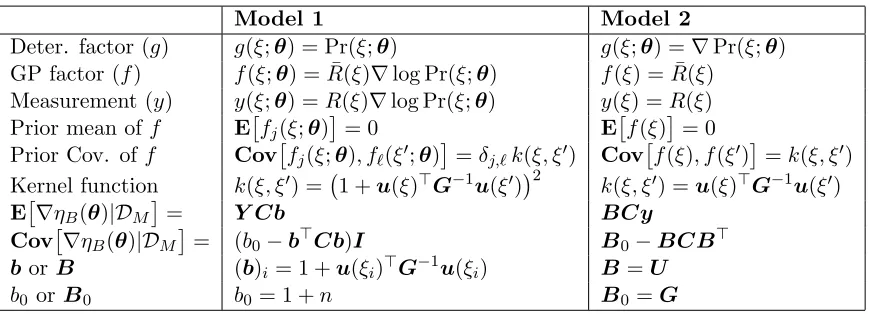
Model 1 Model 2

Deter. factor (g) g(ξ;θ) = Pr(ξ;θ) g(ξ;θ) =∇Pr(ξ;θ) GP factor (f) f(ξ;θ) = ¯R(ξ)∇log Pr(ξ;θ) f(ξ) = ¯R(ξ)

Measurement (y) y(ξ;θ) =R(ξ)∇log Pr(ξ;θ) y(ξ) =R(ξ)

Prior mean off E

fj(ξ;θ)

= 0 E

f(ξ)

= 0

Prior Cov. of f Cov

fj(ξ;θ), f`(ξ0;θ)

=δj,`k(ξ, ξ0) Cov

f(ξ), f(ξ0)

=k(ξ, ξ0) Kernel function k(ξ, ξ0) = 1 +u(ξ)>G−1u(ξ0)2

k(ξ, ξ0) =u(ξ)>G−1u(ξ0) E∇ηB(θ)|DM

= Y Cb BCy

Cov∇ηB(θ)|DM

= (b0−b>Cb)I B0−BCB>

borB (b)i = 1 +u(ξi)>G−1u(ξi) B=U

b0 orB0 b0 = 1 +n B0 =G

Table 1: Summary of the Bayesian policy gradient Models 1 and 2.

Proof See Appendix B.

Table 1 summarizes the two BPG models presented in Sections 4.1 and 4.2. Our choice of Fisher-type kernels was motivated by the notion that a good representation should depend on the process generating the data (see Jaakkola and Haussler, 1999, Shawe-Taylor and Cristianini, 2004, for a thorough discussion). Our particular selection of linear and quadratic Fisher kernels were guided by the desideratum that the posterior moments of the gradient be analytically tractable as discussed in Section 3.

As described above, in either model, we are restricted in the choice of kernel (quadratic Fisher kernel in Model 1 and Fisher kernel in Model 2) in order to be able to derive closed-form expressions for the posterior mean and covariance of the gradient integral. The loss due to this restriction depends on the problem at hand and is hard to quantify. This loss is exactly the loss of selecting an inappropriate prior in any Bayesian algorithm or, more generally, of choosing a wrong representation (function space) in a machine learning algorithm (referred to as approximation error in approximation theory). However, the experimental results of Section 6 indicate that this restriction did not cause a significant error (especially for Model 1) in our gradient estimates, as those estimated by BPG were more accurate than the ones estimated by the MC-based method, given the same number of samples.

4.3 A Bayesian Policy Gradient Evaluation Algorithm

(17)

B. The algorithm then computes the returnRand the measurementy(ξi) for the observed pathξi (Lines 7 and 9), and updates the kernel matrixK (Line 8) using

K :=

K k(ξi) k>(ξi) k(ξi, ξi)

. (28)

Finally, the algorithm adds the measurement errorΣto the covariance matrixK (Line 12) and computes the posterior moments of the policy gradient (Line 14). B(:, i) on Line 10 denotes theith column of the matrixB.

Algorithm 1 A Bayesian Policy Gradient Evaluation Algorithm

1: BPG Eval(θ, M)

• sample size M >0

• a vector of policy parametersθ ∈_Rn

2: SetG=G(θ) , D=∅ 3: fori= 1 to M do

4: Sample a pathξi using the policyµ(θ)

5: D:=DS

{ξi}

6: u(ξi) =PtT=0i−1∇logµ(at,i|xt,i;θ)

7: R(ξi) =PTt=0i−1r(xt,i, at,i)

8: UpdateK using Equation 28

9: y(ξi) =R(ξi)u(ξi) (Model 1) or y(ξi) =R(ξi) (Model 2)

10: (b)i = 1 +u(ξi)>G−1u(ξi) (Model 1) or B(:, i) =u(ξi) (Model 2)

11: end for

12: C = (K+Σ)−1

13: b0= 1 +n (Model 1) or B0=G (Model 2)

14: Compute the posterior mean and covariance of the policy gradient E ∇ηB(θ)|D

=Y Cb , Cov ∇ηB(θ)|D

= (b0−b>Cb)I (Model 1)

or

E ∇ηB(θ)|D

=BCy , Cov ∇ηB(θ)|D

=B0−BCB> (Model 2) 15: return E ∇ηB(θ)|D

and Cov ∇ηB(θ)|D

The kernel functions used in Models 1 and 2 (Equations 23 and 27) are both based on the Fisher kernel. Computing the Fisher kernel requires calculating the Fisher information matrix G(θ) (Equation 24). Consequently, every time we update the policy parameters, we need to recomputeG. In Algorithm 1 we assume that the Fisher information matrix is known. However, in most practical situations this will not be the case, and consequently the Fisher information matrix must be estimated. Let us briefly outline two possible approaches for estimating the Fisher information matrix in an online manner.

1) Monte-Carlo Estimation: The BPG algorithm generates a number of sample paths using the current policy parameterized byθ in order to estimate the gradient∇ηB(θ). We can use these generated sample paths to estimate the Fisher information matrix G(θ) in an online manner, by replacing the expectation inGwith empirical averaging as ˆGM(θ) =

1

M

PM

(18)

(1−ζi) ˆGi+ζiu(ξi)u(ξi)>, whereζiis a step-size withPiζi=∞andPiζi2<∞. Using the Sherman-Morrison matrix inversion lemma, it is possible to directly estimate the inverse of the Fisher information matrix as

ˆ

G−_i₊₁1 = 1 1−ζi

"

ˆ

G−_i 1−ζi ˆ

G_i−1u(ξi) ˆG_i−1u(ξi)> 1−ζi+ζiu(ξi)>Gˆ−_i 1u(ξi)

#

.

2) Maximum Likelihood Estimation: The Fisher information matrix defined by Equa-tion 24 depends on the probability distribuEqua-tion over paths. This distribuEqua-tion is a product of two factors, one corresponding to the current policy and the other corresponding to the MDP’s state-transition probabilityP (see Equation 1). Thus ifP is known, the Fisher infor-mation matrix may be evaluated offline. We can modelP using a parameterized model and then estimate the maximum likelihood (ML) model parameters. This approach may lead to a model-based treatment of policy gradients, which could allow us to transfer information between different policies. Current policy gradient algorithms, including the algorithms described in this paper, are extremely wasteful of training data, since they do not have any

disciplined way to use data collected for previous policy updates in computing the update of the current policy. Model-based policy gradient may help solve this problem.

4.4 BPG Online Sparsification

Algorithm 1 can be made more efficient, both in time and memory, by sparsifying the solution. Such sparsification may be performed incrementally and helps to numerically stabilize the algorithm when the kernel matrix is singular, or nearly so. Sparsification may, in some cases, reduce the accuracy of the solution (the posterior moments of the policy gradient), but it often makes the algorithms significantly faster, especially for large sample sizes. Here we use an online sparsification method proposed by Engel et al. (2002) (see also Csat´o and Opper, 2002) to selectively add a new observed path to a set of dictionary

paths ˜D used as a basis for representing or approximating the full solution. We only add a new path ξi to ˜D, if k(ξi, ξi)−k˜(ξi)>K˜−1k˜(ξi) > τ, where ˜k and ˜K are the dictionary kernel vector and kernel matrix before observingξi, respectively, andτ is a positive threshold parameter that determines the level of accuracy in the approximation as well as the level of sparsity attained. If the new path is added to ˜Dthe dictionary kernel matrix ˜Kis expanded as shown in Equation 28.

Proposition 5 Let K˜ be them×m sparse kernel matrix, where m≤M is the cardinality ofD˜_M. LetAbe theM×mmatrix, whoseith row is [A]_i,_|D˜i|= 1and[A]i,j = 0 ; ∀j6=|

˜

D_i|,

if we add the sample pathξi to the set of sample paths, and bek˜(ξi)>K˜

−1

(19)

are given by

E∇ηB(θ)|DM

=YΣ−1A KA˜ >Σ−1A+I−1˜b

for Model 1

Cov∇ηB(θ)|DM

=

h

(1 +n)−˜b>A>Σ−1A KA˜ >Σ−1A+I−1˜b

i

I

and

E

∇ηB(θ)|DM

= ˜B A>Σ−1AK˜ +I−1

A>Σ−1y

for Model 2

Cov∇ηB(θ)|DM

=G−B A˜ >Σ−1AK˜ +I−1A>Σ−1AB˜>.

Proof See Appendix C.

4.5 A Bayesian Policy Gradient Algorithm

So far we were concerned with estimating the gradient of the expected return with respect to the policy parameters. In this section, we present a Bayesian policy gradient (BPG) al-gorithm that employs the Bayesian gradient estimation methods proposed in Section 4.3 to update the policy parameters. The pseudo-code of this algorithm is shown in Algorithm 2. The algorithm starts with an initial vector of policy parametersθ0, and updates the

param-eters in the direction of the posterior mean of the gradient of the expected return estimated by Algorithm 1. This is repeated N times, or alternatively, until the gradient estimate is sufficiently close to zero.

Algorithm 2 A Bayesian Policy Gradient Algorithm

1: BPG(θ0,β, N, M)

• initial policy parametersθ0 ∈Rn

• learning rates βj , j= 0, . . . , N−1

• number of policy updates N >0

• sample size M >0 for the gradient evaluation algorithm (BPG Eval)

2: forj= 0 to N −1 do

3: ∆θj =E ∇ηB(θj)|DM

from BPG Eval(θj, M)

4: θj+1=θj+βj∆θj (Conventional Gradient)

or

θj+1=θj+βjG(θj)−1∆θj (Natural Gradient)

5: end for

6: return θN

5. Extension to Partially Observable Markov Decision Processes

(20)

of Baxter and Bartlett (2001). In the partially observable case, the stochastic parameterized policyµ(·|·;θ) controls a POMDP, i.e., the policy has access to an observation process that depends on the state, but it may not observe the state itself directly.

Specifically, for each state x∈ X, an observation o∈ O is generated independently ac-cording to a probability distributionPoover observations inO. We denote the probability of observation o at state x by Po(o|x). A stationary stochastic parameterized policy µ(·|·;θ) is a function mapping observations o ∈ O into probability distributions over the actions µ(·|o;θ)∈ P(A). In this case, the probability of a pathξ= (x0, a0, x1, a1, . . . , xT−1, aT−1, xT),

T ∈ {0,1, . . . ,∞}generated by the Markov chain induced by policyµ(·|·;θ) is given by

Pr(ξ;µ) = Pr(ξ;θ) =P0(x0) Z T−1

Y

t=0

Po(ot|xt)µ(at|ot;θ)P(xt+1|xt, at)do0da0. . . doT−1daT−1.

The Fisher score of this path may be written as

u(ξ;θ) =∇log Pr(ξ;θ) = ∇Pr(ξ;θ) Pr(ξ;θ) =

Z T−1 X

t=0

∇logµ(at|ot;θ)

!

do0da0. . . doT−1daT−1,

which is the same as in the observable case (Equation 5), except here the policy is defined over observations instead of states. As a result, the models and algorithms of Section 4 may be used in the partially observable case with no change, substituting observations for states.

Moreover, similarly to the gradient estimated by the GPOMDP algorithm in Baxter and Bartlett (2001), the gradient estimated by Algorithm 1, ∇ηB(θ), may be employed with the conjugate-gradients and line-search methods of Baxter et al. (2001) for making better use of gradient information. This allows us to exploit the information contained in the gradient estimate more aggressively than by simply adjusting the parameters by a small amount in the direction of∇ηB(θ). Conjugate-gradients and line-search are two widely used techniques in non-stochastic optimization that allow us to find better gradient directions than the pure gradient direction, and to obtain better step sizes, respectively.

Note that in this section, we followed Baxter and Bartlett (2001) (the GPOMDP al-gorithm) and considered stochastic policies that map observations to actions. However, as mentioned by Baxter and Bartlett (2001), it is immediate that the same algorithm works for any finite history of observations. Moreover, along the same way that Aberdeen and Baxter (2001) showed that GPOMDP can be extended to apply to policies with internal state, our BPG POMDP algorithm can also be extended to handle such policies.

6. BPG Experimental Results

(21)

Exact MC (10) BQ (10) MC (100) BQ (100)

r(a) =a

1 0

0.995±0.438

−0.001±0.977

0.986±0.050 0.001±0.060

1.000±0.140 0.004±0.317

1.000±0.000001 0.000±0.000004

r(a) =a2

0 2

0.014±1.246 2.034±2.831

0.001±0.082 1.925±0.226

0.005±0.390 1.987±0.857

0.000±0.000003 2.000±0.000011

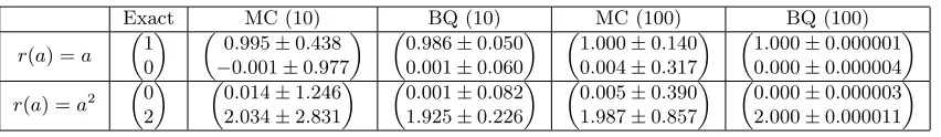
Table 2: The true gradient of the expected return and its MC and BQ estimates for two instances of the bandit problem corresponding to two different reward functions.

System: Policy:

Initial State: x0 ∼ N(0.3,0.001) Actions: at∼µ(·|xt;θ) =N(λxt, σ2)

Reward: rt=x2t + 0.1a2t Parameters: θ= (λ , σ)> Transition: xt+1 =xt+at+nx ; nx ∼ N(0,0.01)

6.1 A Simple Bandit Problem

The goal of this example is to compare the BQ and MC estimates of the gradient (for some fixed set of policy parameters) using the same sample. Our bandit problem has a single state and a continuous action spaceA=R, thus, each pathξi consists of a single actionai. The

policy, and therefore also the distribution over the paths is given bya∼ N(θ1 = 0, θ22 = 1).

The parameters θ1 and θ2 are the mean and the standard deviation of this distribution.

The score function of the path ξ=a and the Fisher information matrix for the policy are u(ξ) = [a, a2−1]> andG= diag(1,2), respectively.

Table 2 shows the exact gradient of the expected return and its MC and BQ estimates using 10 and 100 samples for two instances of the bandit problem corresponding to two different deterministic reward functions r(a) =aandr(a) =a2_{. The average over 10}4 _runs

of the MC and BQ estimates and their standard deviations are reported in Table 2. The true gradient is analytically tractable and is reported as “Exact” in Table 2 for reference.

As shown in Table 2, the variance of the BQ estimates are lower than the variance of the MC estimates by an order of magnitude for the small sample size (M = 10), and by 6 orders of magnitude for the large sample size (M = 100). The BQ estimate is also more accurate than the MC estimate for the large sample size, and is roughly the same for the small sample size.

6.2 Linear Quadratic Regulator

In this section, we consider the following linear system in which the goal is to minimize the expected return over 20 steps.14 Thus, it is an episodic problem with paths of length 20.

We run two sets of experiments on this system. We first fix the set of policy parameters and compare the BQ and MC estimates of the gradient of the expected return using the same sample. We then proceed to solving the complete policy gradient problem and compare the performance of the BPG algorithm (with both conventional and natural gradients) with a Monte-Carlo based policy gradient (MCPG) algorithm.

(22)

0 20 40 60 80 100 102

103 104 105

Number of Paths (M)

Mean Squared Error

MC BQ

0 20 40 60 80 100

0 10 20 30 40 50 60 70

Mean Absolute Angular Error (deg)

MC BQ

0 20 40 60 80 100

102

103

104

105

MC BQ

0 20 40 60 80 100

0 10 20 30 40 50 60 70

MC BQ

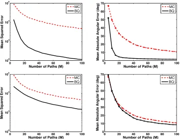
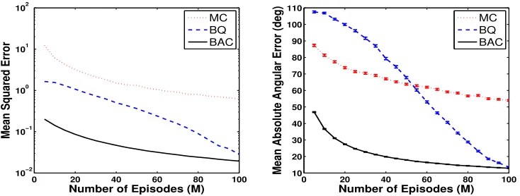
Figure 1: Results for the LQR problem using Model 1 (top row) and Model 2 (bottom row) with sparsification. Shown are the MSE (left column) and the mean absolute angular error (right column) of the MC and BQ estimates as a function of the number of sample pathsM. All results are averaged over 104 runs.

6.2.1 Gradient Estimation

In this section, we compare the BQ and MC estimates of the gradient of the expected return for the policy induced by parameters λ=−0.2 andσ = 1. We use several different sample sizes (number of paths used for gradient estimation) M = 5j , j = 1, . . . ,20 for the BQ and MC estimates. For each sample size, we compute the MC and BQ estimators using the same sample, repeat this process 104 times, and then compute the average. The true gradient is analytically tractable and is used for comparison purposes.

Figure 1 shows the mean squared error (MSE) (left column) and the mean absolute angular error (right column) of the MC and BQ estimates of the gradient for several different sample sizes. The absolute angular error is the absolute value of the angle between the true and estimated gradients. In this figure, the BQ gradient estimates were calculated using Model 1 (top row) and Model 2 (bottom row) with sparsification. The error bars in the figures on the right column are the standard errors of the mean absolute angular errors.

We ran another set of experiments in which we added i.i.d. Gaussian noise to the rewards:

(23)

of f(ξ), is of the form R(ξ)∇log Pr(ξ;θ) and R(ξ), respectively (see Sections 4.1 and 4.2). Moreover, since each rewardrtis a Gaussian random variable with variance σ2_r, the return R(ξ) =PT−1

t=0 rt is also a Gaussian random variable with variance T σr2. Therefore in this case, the measurement noise covariance matrices for Models 1 and 2 may be written asΣ=

T σ2

rdiag

∂

∂θilogp(ξ1;θ)

2

, . . . , _∂θ∂

ilogp(ξM;θ)

2

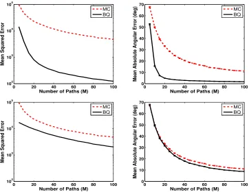
andΣ=T σ2_rI, respectively, whereT = 20 is the path length.15 We tried two different Gaussian reward noise standard deviations: σr = 0.1 and 1 in our experiments. Adding noise to the rewards slightly increased the error of the BQ and MC estimates of the gradient. However, the graphs comparing these estimates remained quite similar to those shown in Figure 1. Hence in Figure 2, we compare the MSE (left column) and the mean absolute angular error (right column) of the BQ estimates with and without noise in the rewards as a function of the number of sample paths M. In this figure, the noise in the rewards has variance σ_r2 = 1, and the BQ gradient estimates were calculated using Model 1 (top row) and Model 2 (bottom row) with sparsification.

6.2.2 Policy Optimization

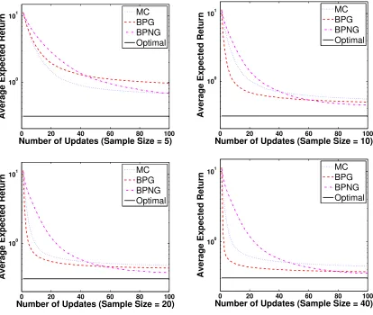
In this section, we use Bayesian policy gradient (BPG) to optimize the policy parameters in the LQR problem. Figure 3 shows the performance of the BPG algorithm with the conventional (BPG) and natural (BPNG) gradient estimates, versus a MC-based policy gradient (MCPG) algorithm, for sample sizes (number of sample paths used to estimate the gradient of each policy) M = 5, 10, 20, and 40. We use Algorithm 2 with the number of updates set toN = 100, and Model 1 with sparsification for the BPG and BPNG methods. Since Algorithm 2 computes the Fisher information matrix for each set of policy parameters, the estimate of the natural gradient is provided at little extra cost at each step. The returns obtained by these methods are averaged over 104runs. The policy parameters are initialized randomly at each run. In order to ensure that the learned parameters do not exceed an acceptable range, the policy parameters are defined as λ= −1.999 + 1.998/(1 +eκ1) and σ = 0.001 + 1/(1 +eκ2). The optimal solution is λ∗ ≈ −0.92, σ∗ = 0.001, ηB(λ∗, σ∗) = 0.3067, corresponding to κ∗₁ ≈ −0.16 and κ∗₂→ ∞.

Figure 3 shows that the MCPG algorithm performs better than BPG and BPNG only for the smallest sample size (M = 5), whereas for larger samples BPG and BPNG dominate MCPG. The better performance of MCPG for very small sample size is due to the fact that in this case, the Bayesian estimators, BPG and BPNG, like any other Bayesian estimator or posterior in such case, rely more on the prior, and thus, are not accurate if the prior is not very informative. A similar phenomenon was also reported by Rasmussen and Ghahramani (2003). We used two different learning rates for the two components of the gradient. For a fixed sample size, BPG and MCPG methods start with an initial learning rate and decrease it according to the schedule βj = β0 20/(20 +j)

. The BPNG algorithm uses a fixed learning rate multiplied by the determinant of the Fisher information matrix. We tried many values for the initial learning rates used by these algorithms and those in Table 3 yielded the best performance of those we tried.

So far we have assumed that the Fisher information matrix is known. In the next experiment, we estimate it using both MC and a model-based maximum likelihood (ML)

15. In Model 1,Σis the measurement noise covariance matrix for theith component of the gradient ∂

∂θiηB(θ).

Note that ∂

(24)

0 20 40 60 80 100

102

103

104

105

MC BQ

0 20 40 60 80 100

0 10 20 30 40 50 60 70

MC BQ

0 20 40 60 80 100

102

103

104

105

MC BQ

0 20 40 60 80 100

0 10 20 30 40 50 60 70

MC BQ

Figure 2: Results for the LQR problem in which the rewards are corrupted by i.i.d. Gaus-sian noise withσ2_r = 1. Shown are the MSE (left column) and the mean absolute angular error (right column) of the BQ estimates with and without noise in the rewards as a function of the number of sample paths M. The BQ gradient esti-mates were calculated using Model 1 (top row) and Model 2 (bottom row) with sparsification. All results are averaged over 104 runs.

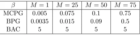
β0 M = 5 M = 10 M = 20 M = 40

MCPG 0.01,0.05 0.05,0.05 0.05,0.10 0.05,0.10 BPG 0.01,0.05 0.07,0.10 0.15,0.15 0.10,0.30 BPNG 0.010,0.005 0.010,0.005 0.015,0.005 0.015,0.005 BPG-var 0.05,0.05 0.10,0.10 0.10,0.15 0.15,0.30

Table 3: Initial learning rates β0 used by the policy gradient algorithms for the two

com-ponents of the gradient.

method, as discussed in Section 4.3. In the ML approach, we model the transition proba-bility function asP(xt+1|xt, at) =N(c1xt+c2at+c3, c24), and then estimate its parameters

(c1, c2, c3, c4) using observing state transitions. Figure 4 shows that the BPG algorithm,

(25)

bet-0 20 40 60 80 100 100

101

Number of Updates (Sample Size = 5)

Average Expected Return

MC BPG BPNG Optimal

0 20 40 60 80 100

100 101

MC BPG BPNG Optimal

0 20 40 60 80 100

100 101

MC BPG BPNG Optimal

0 20 40 60 80 100

100 101

MC BPG BPNG Optimal

Figure 3: A comparison of the average expected returns of the Bayesian policy gradient al-gorithm using conventional (BPG) and natural (BPNG) gradient estimates, with the average expected return of a MC-based policy gradient algorithm (MCPG) for sample sizesM = 5, 10, 20, and 40. All results are averaged over 104 runs.

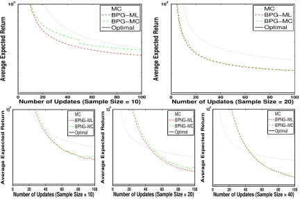
ter than MCPG. Top and bottom rows contain the results for the BPG algorithm with conventional (BPG-ML and BPG-MC) and natural (BPNG-ML and BPNG-MC) gradi-ent estimates, respectively. Although the BPG-ML (BPNG-ML) outperforms BPG-MC (BPNG-MC) for small sample sizes, the difference in their performance disappears as we increase the sample size. One reason for the good performance of BPG-ML is that the form of the state transition functionP(xt+1|xt, at) has been selected correctly. Here we used the same initial learning rates and learning rate schedules as in the experiments of Figure 3 (see Table 3).

(26)

0 20 40 60 80 100 100

MC BPG−ML BPG−MC Optimal

0 20 40 60 80 100

100

MC BPG−ML BPG−MC Optimal

0 20 40 60 80 100 100

MC BPNG−ML BPNG−MC Optimal

0 20 40 60 80 100 100

Figure 4: A comparison of the average expected returns of the BPG algorithm, when the Fisher information matrix is estimated using ML and MC, with the average ex-pected return of a MC-based policy gradient algorithm (MCPG). The top and bottom rows contain the results for the BPG algorithm with conventional (BPG-ML and BPG-MC) and natural (BPNG-(BPG-ML and BPNG-MC) gradient estimates, respectively. All results are averaged over 104 runs.

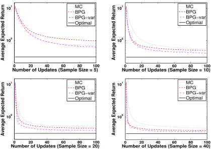
second moment information provided by the Bayesian policy gradient estimation algorithm (Algorithm 1). In the last experiment of this section, we use the posterior covariance of the gradient, provided by Algorithm 1, to select the learning rate and the direction of the updates in Algorithm 2. The idea is to use a small learning rate when the variance of the gradient estimate is large, and to have a large update when it is small. We refer to the resulting algorithm by the name BPG-var. This algorithm uses a fixed learning rate parameter (see Table 3) multiplied by

h

1+nI−Cov ∇ηB(θ)|DM

i

/(1+n) in its updates. Note thatn+ 1 is b0 in the calculation of the posterior covariance of the gradient in Model

(27)

0 20 40 60 80 100 100

101

MC BPG BPG−var Optimal

0 20 40 60 80 100

100 101

0 20 40 60 80 100

100 101

0 20 40 60 80 100

100 101

Figure 5: A comparison of the average expected returns of the BPG algorithm that uses the posterior covariance in its updates (BPG-var), with the average expected return of the BPG and a MC-based policy gradient algorithm (MCPG) for sample sizes M = 5, 10, 20, and 40. All results are averaged over 104 runs.

BPG-var converges faster than BPNG and has similar final performance. As we expected, BPG-var and BPG perform more and more alike as we increase the sample size. This is because by increasing the sample size the estimated gradient (the posterior mean of the gradient), and as a result, the update direction used by BPG becomes more reliable.

In an approach similar to the one used in the experiments of Figure 5, Vien et al. (2011) used BQ to estimate the Hessian matrix distribution, and then used its mean as learning rate schedule to improve the performance of BPG. They empirically showed that their method performs better than BPG and BPNG in terms of convergence speed.

7. Bayesian Actor-Critic