Eigenvalue Methods for Interpolation Bases

(1)

Western University Western University

Scholarship@Western

Electronic Thesis and Dissertation Repository

7-8-2013 12:00 AM

Eigenvalue Methods for Interpolation Bases

Piers W. Lawrence

The University of Western Ontario Supervisor

Corless, Robert M.

The University of Western Ontario

Graduate Program in Applied Mathematics

A thesis submitted in partial fulfillment of the requirements for the degree in Doctor of Philosophy

Follow this and additional works at: https://ir.lib.uwo.ca/etd Part of the Numerical Analysis and Computation Commons

Recommended Citation Recommended Citation

Lawrence, Piers W., "Eigenvalue Methods for Interpolation Bases" (2013). Electronic Thesis and Dissertation Repository. 1359.

https://ir.lib.uwo.ca/etd/1359

(2)

Eigenvalue Methods for Interpolation Bases

(Thesis format: Integrated-Article)

by

Piers William Lawrence

Graduate Program in Applied Mathematics

A thesis submitted in partial fulfillment

of the requirements for the degree of

Doctor of Philosophy

The School of Graduate and Postdoctoral Studies

The University of Western Ontario

London, Ontario, Canada

(3)

Abstract

This thesis investigates eigenvalue techniques for the location of roots of poly-nomials expressed in the Lagrange basis. Polynomial approximations to

func-tions arise in almost all areas of computational mathematics, since polynomial

expressions can be manipulated in ways that the original function cannot.

Polynomials are most often expressed in the monomial basis; however, in many

applications polynomials are constructed by interpolating data at a series of

points. The roots of such polynomial interpolants can be found by computing

the eigenvalues of a generalized companion matrix pair constructed directly

from the values of the interpolant. This affords the opportunity to work with

polynomials expressed directly in the interpolation basis in which they were posed, avoiding the often ill-conditioned transformation between bases.

Working within this framework, this thesis demonstrates that computing

the roots of polynomials via these companion matrices is numerically stable,

and the matrices involved can be reduced in such a way as to significantly

lower the number of operations required to obtain the roots.

Through examination of these various techniques, this thesis offers insight

into the speed, stability, and accuracy of rootfinding algorithms for

polynomi-als expressed in alternative bases.

Keywords: polynomial interpolation, Lagrange interpolation, barycentric

formula, generalized companion matrices, polynomial roots, eigenvalue

prob-lem, stability, backward error, semiseparable matrices, nonlinear eigenvalue

(4)

Co-Authorship Statement

Chapters 3 and 4 were co-authored with Rob Corless, and have been submit-ted for publication. Rob Corless supervised the research, and provided key

guidance for the formulation and proof of the main theorem of Chapter 3.

(5)

Acknowledgements

Although there may have been many opportunities for this thesis not to have come to fruition, it has, and I am grateful to many people who have made this

possible.

First of all, had it not been for Rob Corless, none of this would have been

possible. It was his visit to the University of Canterbury, at the precise moment

I was contemplating pursuing a PhD, and his inspiring talk on barycentric

Hermite interpolation which started the ball rolling. I would like to thank

him for the many discussions we have had, and his patience explaining the

intricacies of backward error analysis.

From the Department, I would like to thank Colin Denniston for always having an open door, and a willingness to discuss any topic of mathematics.

I also thank him for providing the funds for our departmental morning teas,

making the department feel a little more like home. I also thank David Jeffrey

for sharing many humorous anecdotes, and his expert editorial advice.

Further abroad, I would like to thank Georges Klein, for the many

stimu-lating discussions about barycentric interpolation, and for inviting me to visit

Fribourg to work on rootfinding problems relating to Floater-Hormann

inter-polation.

From the University of Canterbury, I thank Chris Hann for showing me the path into mathematics and into research—I may well have become an engineer

otherwise. I thank Bob Broughton and Mark Hickman for their stellar teaching

and mentorship, and for sparking my interest in numerical linear algebra and

numerical computation.

(6)

experience more interesting, not least of all James Marshall, for the many

discussions on any topic you wish to name. I thank Frances, Mona, Melissa,

Alex, Walid, Bernard, and Anna for providing good companionship. I also

thank Dave and Aimee for the excellent BBQ, and for exposing me to the

beauty of the cottage in Canada.

To my parents, I thank them for supporting me in my endeavours into

mathematics, even though these pursuits have taken me out of middle earth

to the other side of the world.

Above all I thank Trish for her constant and unwavering love and support.

(7)

List of Tables

2.1 Maximum error in computed eigenvalues for Wilkinson’s

poly-nomial, sampled at different node distributions. . . 39

2.2 Measure of loss of orthogonality of vectors q0, . . . ,qn produced

from the Lanczos type reduction process of §2.2.1. . . 39

2.3 Leading coefficients of the degree six interpolant to (2.87). . . 40

2.4 Leading coefficients of the degree 11 interpolant to (2.88). . . . 41

2.5 Elements of c1 produced by the Givens type reduction process. 42

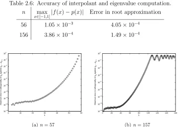
2.6 Accuracy of interpolant and eigenvalue computation. . . 44

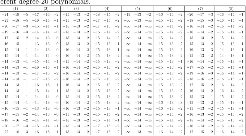
3.1 Relative backward error in coefficients (log base 10) for eight

different degree-20 polynomials. . . 63

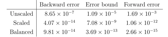
3.2 Maximum observed backward error and bound. . . 63

3.3 Wilkinson polynomial interpolated at equispaced points. . . . 68

3.4 Wilkinson polynomial interpolated at Chebyshev points. . . . 69

(11)

List of Figures

2.1 Distribution of maximum error in the subdiagonal entries of T. 36

2.2 Maximum forward error in the computed roots from each of the

four reduction processes. . . 37

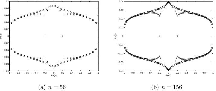
2.3 Roots (+) and poles (◦) of the rational interpolant. . . 43

2.4 Error in orthogonality of vectorsq0, . . . ,qn: max 0≤i≤k−1|q ∗ iqk|. . . 44

3.1 Chebyshev polynomials interpolated at their extreme points. . 65

3.2 Polynomials taking on random normally distributed values at Chebyshev nodes of the first kind. . . 66

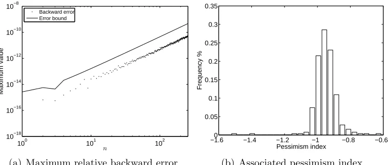
3.3 Backward error and bound for 10000 degree 50 polynomials tak-ing on random normally distributed values at Chebyshev points of the first kind. . . 66

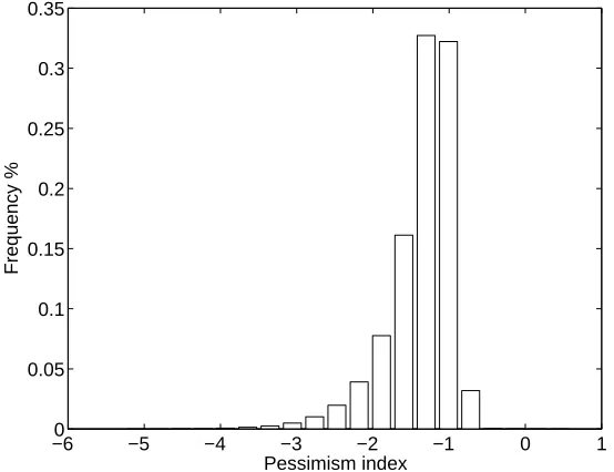
3.4 Pessimism index for 10000 degree 50 polynomials taking on ran-dom normally distributed values at Chebyshev points of the first kind. . . 67

4.1 Butterfly example, eigenvalue distribution. . . 90

4.2 Butterfly example, backward error distributions. . . 91

4.3 Butterfly example, pessimism index distributions. . . 91

4.4 Speaker enclosure example, eigenvalue distribution. . . 92

4.5 Speaker enclosure example, backward error distributions. . . . 93

4.6 Damped mass spring system, eigenvalue distribution. . . 94

4.7 Damped mass spring system, backward error distributions. . . 94

4.8 Damped mass spring system, pessimism index distributions. . 95

4.9 Damped gyroscopic system, distributions of eigenvalues and pseudospectra. The dotted line represents the level curve where BM(z) = BL(z). . . 96

4.10 Damped gyroscopic system, backward error distributions. . . . 97

(12)

List of Algorithms

1 Reduction of A to symmetric tridiagonal plus rank-one form. . 105

(13)

List of Notation

adj(A) The adjugate of A: the transpose of the cofactor

matrix of A.

[zn_](_p₍_z₎₎ _{Coefficient of} _zn _{of the polynomial} _p₍_z_).

kAkF Frobenius norm ofA defined by

kAkF =

v u u t

n

X

i=1

n

X

j=1

|aij|2

k(A,B)kF Frobenius norm of the matrix pair(A,B) defined

by

k(A,B)kF =

q

kAk2

F +kBk2F .

η(A,B)(λ,z) Backward error of an approximate eigenpair (λ,z)

of the linearization (A,B).

ηP(λ,x) Backward error of an approximate eigenpair (λ,x)

(14)

Chapter 1 Introduction

1.1 Motivation

Solving univariate polynomial equations is an essential part of numerical

anal-ysis, and for a great many other areas in mathematics. It is well known that

the accuracy of computing the roots of univariate polynomials is strongly

af-fected by the basis in which the polynomial is originally expressed. Yet, most

classical polynomial rootfinders require that polynomials be converted to the monomial basis first, before calling the rootfinder. Significant exceptions to

this approach include the rootfinder used in the software package Chebfun

[26] which is based upon the Chebyshev Colleague matrix [14, 22]; the

al-gorithm proposed by Day and Romero [10] for orthogonal polynomial bases;

and the Bernstein-B´ezier package of Farouki and Rajan [12]. Conversion to

another basis cannot be expected to improve the numerical conditioning of

the polynomial, and indeed such conversion usually makes it much worse—

exponentially worse, in the degree [15]. Therefore, conversion between bases

should be avoided.

In this thesis, we explore the computation of the roots of polynomials via

eigenvalue methods. Instead of solving the polynomial equation directly, we

linearize the polynomial, which is to say the polynomial is transformed into a

generalized eigenvalue problem whose eigenvalues are exactly the roots of the

(15)

may be computed via the Frobenius companion matrix constructed from the

polynomial coefficients. Working in the barycentric Lagrange basis has

signifi-cant accuracy advantages [4, 9]. According to Higham [17], the first form of the

barycentric interpolation formula is backward stable, and the second

barycen-tric form is forward stable for any set of nodes with a small Lebesgue constant.

The particular linearization we investigate is the generalized companion

ma-trix pair first proposed by Corless [6], constructed from the coefficients of the

polynomial in the Lagrange basis.

Forming the linearization of a polynomial has the effect of squaring the

number of values involved: the generalized eigenvalue problem involves O(n2) entries. Furthermore, the complexity of computing the eigenvalues (via the

QZ algorithm) is an O(n3_{) process.} _{As pointed out by Moler [21], many}

people are willing to pay theO(n3_{) cost of this approach simply because of its}

convenience. Here we give a proof of the stability, and lower the cost.

In the literature to date, this particular linearization has been used in

practice before any rigorous analysis of its stability has been conducted.

Ac-cordingly, one of the primary objectives of this thesis is to examine the stability

properties of this linearization. Most studies investigating the stability

prop-erties of computing roots of polynomials via linearization consider only the monomial basis. The advantages of using the Lagrange basis for computations

are significant, and thus there is a need to address the corresponding stability

properties of rootfinding via linearization for the Lagrange basis.

To discuss the stability properties we first introduce the notion of condition

numbers and backward errors, further details can be found in [8]. Consider

the situation where we wish to compute the value of a function y = f(x)

for some given x. Lets say we have an algorithm that computes a solution _by

approximating y. We ask the question: for what input data have we actually

solved our problem? Or in other words for what perturbation δx is y_b =

f(x +δx) satisfied? The backward error is then just the smallest |δx| for

which the equation _by=f(x+δx) is satisfied. The forward error is measured

by the difference between the approximate solution and the true solution of

(16)

through the condition number, in general we have the relationship

Forward error ≤Condition number×Backward error. (1.1)

Thus, an algorithm is called backward stable if the backward error is small,

because the backward error and condition number provide a bound on the

forward error. If the problem which we are solving is well-conditioned, and the small backward error is small, then the forward error will also be small.

Furthermore, we are motivated by applications that give rise to polynomial

eigenvalue problems, or matrix polynomials. We find significant discussion of

the quadratic eigenvalue problem (QEP) in [24], a problem which has received

much attention in recent years because of the vast variety of application areas

that give rise to QEPs, including dynamical analysis of mechanical systems,

acoustics, and linear stability of flows in fluid mechanics, to name a few.

Sim-ilarly, higher order polynomial eigenvalue problems also arise in a number of

application areas. It is not entirely clear that the monomial basis is the best basis for expressing matrix polynomials, and the Lagrange basis may yet prove

to be superior for formulating and solving high-order matrix polynomials.

Born out of the need to produce accurate and stable numerical methods

for solving the polynomial eigenvalue problem, this thesis addresses the

mat-ter of the numerical stability of computing eigenpairs of matrix polynomials

expressed in the Lagrange basis. We demonstrate the conditions under which

eigenpairs, computed via linearization of matrix polynomials, are numerically

stable. We also show, through numerical examples, that by applying

block-wise balancing to the linearization we are able to compute eigenpairs with small backward errors, and give computable and intelligible upper bounds for

the backward errors.

One might ask why not just use Newton’s method to compute the roots?

The answer to this is that we wish to compute all of the roots, not just a

selection. The eigenvalue techniques discussed in this thesis are robust and

convenient for just this task. Therefore, we start there and modify the them

(17)

1.2 Outline

Chapter 2 investigates the structured reduction of the linearization of scalar

polynomials expressed in the Lagrange basis. The linearization we investigate

has only O(n) nonzero entries, and is a low-rank perturbation of a diagonal

matrix. It is our goal to retain some sort of structure of the linearization during

the solution process. Normally the eigenvalue problem is reduced first to upper

Hessenberg form to reduce the complexity of carrying out QZ iterations. For real interpolation nodes, the Hessenberg form also has low-rank structure,

being a rank one perturbation of a symmetric tridiagonal matrix. Thus, we

should be able to transform the original linearization to another low-rank

formulation. We show that such a transformation may be achieved in only

O(n2_{) operations, by applying structured methods. Furthermore, once we have}

reduced the matrix to tridiagonal plus rank one form, there exist a variety of

O(n2) methods to apply the QR algorithm to the matrix. Hence, we could

obtain an O(n2) algorithm for locating all n roots of the original polynomial. In Chapter 3, we investigate the stability of computing roots of polynomi-als via linearization. In the monomial basis, the conditions under which the

Frobenius companion matrix produces accurate and stable roots of the

poly-nomial has been established in [11]. For the Lagrange basis, the corresponding

analysis is lacking, and filling this gap in the literature is one of the

contribu-tions that this thesis offers. We obtain bounds on the backward error that are

easily computable and intelligible. Through a range of numerical experiments,

we illustrate that the backward error is small, and that the bound is often only

around one order of magnitude larger than the actual backward error. We also

develop a balancing strategy for the linearization, to improve the accuracy of

the computed eigenvalues.

In Chapter 4, we investigate the stability of computing eigenvalues and

eigenvectors of matrix polynomials expressed in the Lagrange basis via

lin-earization. We establish the conditions under which the linearization

pro-duces eigenpairs with small backward errors, and provide computable bounds

(18)

similar to that for the scalar case, we are able to compute eigenpairs with

excellent backward errors for a range of numerical examples, and our bounds

are approximately one order of magnitude larger.

In sum, this thesis offers new algorithms for the structured reduction of

linearizations of polynomials in the Lagrange basis, and undertakes the

nec-essary analysis to establish the numerical stability of computing roots and

eigenvalues of polynomials and matrix polynomials.

1.3 A Brief Literature Review

The literature on polynomial rootfinding is vast, and we do not aim to be

exhaustive. Much of literature on solving polynomial equations can be found

in the electronic bibliographies authored by McNamee [18, 19]. Also the book

[20] by the same author contains an extensive overview of methods for solving

univariate polynomials. Various matrix methods for solving univariate

poly-nomial equations have been proposed. Much of the framework for working in

the Lagrange basis has been described in [1, 6]. The necessary extensions to

matrix polynomials can be found in [2, 7]. Both of these references provide a good grounding for what has been done so far in the Lagrange basis, as well

as the book [8] which has many discussions about alternative bases, as well

as significant discussion on backward error. Other matrix approaches have

been proposed in the Lagrange basis, these may be found in [5] and the

refer-ences therein. For the Chebyshev basis the appropriate results can be found

in [14, 22]. For matrix methods for other orthogonal polynomial bases, many

results may be found in [10].

For a good introduction to barycentric Lagrange interpolation, we point to

the landmark paper by Berrut and Trefethen [4]. We also point out Trefethen’s book on approximation theory [25] as a good introduction to polynomial

in-terpolation. There have been a number of recent papers discussing the various

properties of the barycentric Lagrange formulation. For a good overview, we

suggest [3, 17, 27].

(19)

many backward stability results (in the Monomial basis), we refer to [16, 23].

Bibliography

[1] A. Amiraslani, R. M. Corless, L. Gonzalez-Vega,

and A. Shakoori, Polynomial algebra by values, Tech. Rep.

TR-04-01, Ontario Research Centre for Computer Algebra,

http://www.orcca.on.ca/TechReports, January 2004.

[2] A. Amiraslani, R. M. Corless, and P. Lancaster, Linearization

of matrix polynomials expressed in polynomial bases, IMA Journal of

Nu-merical Analysis, 29 (2009), pp. 141–157.

[3] J.-P. Berrut, R. Baltensperger, and H. D. Mittelmann,Recent

developments in barycentric rational interpolation, in Trends and

appli-cations in constructive approximation, Springer, 2005, pp. 27–51.

[4] J.-P. Berrut and L. N. Trefethen, Barycentric Lagrange

interpo-lation, SIAM Review, 46 (2004), pp. 501–517.

[5] D. Bini, L. Gemignani, and V. Pan, Fast and stable QR eigenvalue

algorithms for generalized companion matrices and secular equations,

Nu-merische Mathematik, 100 (2005), pp. 373–408.

[6] R. M. Corless,Generalized companion matrices in the Lagrange basis, in Proceedings EACA, L. Gonzalez-Vega and T. Recio, eds., June 2004, pp. 317–322.

[7] , On a generalized companion matrix pencil for matrix

polynomi-als expressed in the Lagrange basis, in Symbolic-Numeric Computation,

D. Wang and L. Zhi, eds., Trends in Mathematics, Birkhuser Basel, 2007, pp. 1–15.

[8] R. M. Corless and N. Fillion,A graduate survey of numerical meth-ods, Forthcoming, 2014, (2014).

[9] R. M. Corless and S. M. Watt, Bernstein bases are optimal,

but, sometimes, Lagrange bases are better, in Proceedings of SYNASC,

Timisoara, MIRTON Press, September 2004, pp. 141–153.

[10] D. Day and L. Romero, Roots of polynomials expressed in terms of

orthogonal polynomials, SIAM Journal on Numerical Analysis, 43 (2005),

(20)

[11] A. Edelman and H. Murakami, Polynomial roots from companion

matrix eigenvalues, Mathematics of Computation, 64 (1995), pp. 763–

776.

[12] R. T. Farouki and V. T. Rajan,Algorithms for polynomials in

Bern-stein form, Comput. Aided Geom. Des., 5 (1988), pp. 1–26.

[13] I. Gohberg, P. Lancaster, and L. Rodman, Matrix polynomials, SIAM, 2009.

[14] I. J. Good,The Colleague matrix, a Chebyshev analogue of the

compan-ion matrix, The Quarterly Journal of Mathematics, 12 (1961), pp. 61–68.

[15] T. Hermann, On the stability of polynomial transformations between

Taylor, Bernstein and Hermite forms, Numerical Algorithms, 13 (1996),

pp. 307–320.

[16] N. Higham, R. Li, and F. Tisseur, Backward error of polynomial

eigenproblems solved by linearization, SIAM Journal on Matrix Analysis

and Applications, 29 (2008), pp. 1218–1241.

[17] N. J. Higham, The numerical stability of barycentric Lagrange

interpo-lation, IMA Journal of Numerical Analysis, 24 (2004), pp. 547–556.

[18] J. M. McNamee, A bibliography on roots of polynomials, Journal of Computational and Applied Mathematics, 47 (1993), pp. 391–394.

[19] , A 2002 update of the supplementary bibliography on roots of

poly-nomials, J. Comput. Appl. Math., 142 (2002), pp. 433–434.

[20] J. M. McNamee, Numerical methods for roots of polynomials. Part I, Elsevier Science, 2007.

[21] C. Moler, Cleves corner: Roots—of polynomials, that is, The Math-Works Newsletter, 5 (1991), pp. 8–9.

[22] W. Specht,Die Lage der Nullstellen eines Polynoms. III, Mathematis-che Nachrichten, 16 (1957), pp. 369–389.

[23] F. Tisseur,Backward error and condition of polynomial eigenvalue prob-lems, Linear Algebra and its Applications, 309 (2000), pp. 339–361.

(21)

[25] L. N. Trefethen, Approximation theory and approximation practice, Society for Industrial and Applied Mathematics, 2012.

[26] L. N. Trefethen et al.,Chebfun Version 4.2, The Chebfun

Develop-ment Team, 2011. http://www.maths.ox.ac.uk/chebfun/.

[27] M. Webb, L. N. Trefethen, and P. Gonnet, Stability of

barycen-tric interpolation formulas for extrapolation, SIAM Journal on Scientific

(22)

Chapter 2 Fast Reduction of Generalized

Companion Matrix Pairs for

Barycentric Lagrange

Interpolants

1

2.1 Introduction

For a polynomial p(z) expressed in the monomial basis, it is well known that

one can find the roots of p(z) by computing the eigenvalues of a certain

com-panion matrix constructed from its coefficients. For polynomials expressed in

other bases (such as the Chebyshev basis, the Lagrange basis, or other

or-thogonal polynomial bases), generalizations of the companion matrix exist,

constructed from the appropriate coefficients; see for example [4, 5, 10, 21].

In this article we consider polynomial interpolants in the Lagrange basis,

expressed in barycentric form. Berrut and Trefethen [2] present a

comprehen-sive review of such polynomial interpolants.

Given a set of n+ 1 distinct interpolation nodes {x0, . . . , xn}, with

corre-1_{A version of this chapter has been submitted to the SIAM Journal of Matrix Analysis}

(23)

sponding values {f0, . . . , fn}, the barycentric weights wj are defined by

wj = n

Y

k=0

k6=j

(xj −xk)−1, 0≤j ≤n . (2.1)

The unique polynomial of degree less than or equal toninterpolating the data

fj at xj is

p(z) =

n

Y

i=0

(z−xi) n

X

j=0

wj

(z−xj)

fj . (2.2)

Equation (2.2) is known as the “first form of the barycentric interpolation

formula” [20] or the “modified Lagrange formula” [12]. The “second (true)

form of the barycentric formula” [20] is

p(z) =

n

X

j=0

wj

(z−xj)

fj n

X

j=0

wj

(z−xj)

, (2.3)

which is constructed by dividing Equation (2.2) by the interpolant of the con-stant function 1 at the same nodes, and by cancelling the factorQn

i=0(z−xi).

As was first shown in [4], the roots of the interpolating polynomial p(z),

as defined by (2.2), are exactly the generalized eigenvalues of the matrix pair

(A,B) =

"

0 −fT

w D # , " 0 I #! , (2.4)

where w=h w0 · · · wn

iT

, fT ₌h _f

0 · · · fn

i , and D =     x0 . .. xn     . (2.5)

(24)

i, 0≤i≤n, then

det (zB−A) = det

"

0 fT

−w zI−D

#

(2.6)

= det (zI−D) det 0 +fT (zI−D)−1w

(2.7)

=

n

Y

i=0

(z−xi) n

X

j=0

wjfj

(z−xj)

=p(z), (2.8)

and then by continuity at z = xi we have det (zB−A) = p(z). Thus, the

eigenvalues of the matrix pair (A,B) are exactly the roots of p(z).

Further-more, computing the roots of polynomial interpolants via the eigenvalues of

the matrix pair (A,B) is numerically stable, as shown in Chapter 3 and in

[14].

Remark 1. While the degree of the polynomial interpolantp(z)is less than or

equal to n, the dimensions of the matrices A and B are n+ 2 by n+ 2. This

formulation gives rise to two spurious infinite eigenvalues. We will show how

to deflate these infinite eigenvalues in §2.3.3.

The second form of the barycentric interpolation formula has a remarkable

feature [1]: the interpolating property is satisfied independently of the choice of weights wj, as long as they are all nonzero. Let us define some arbitrary

nonzero weightsuj, we may write a rational interpolant as a quotient of

poly-nomials interpolating the values ukfk/wk and uk/wk at the nodes xk, where

the wk’s are the weights given in (2.1). The rational function is then given by

r(z) =

n

Y

i=0

(z−xi) n

X

j=0

wj

(z−xj)

ujfj

wj

n

Y

i=0

(z−xi) n

X

j=0

wj

(z−xj)

uj

wj

(25)

or

r(z) =

n

X

j=0

uj

(z−xj)

fj n

X

j=0

uj

(z−xj)

, (2.10)

which is exactly the second barycentric formula for the weightsuk. The choice

of weights (2.1) forces the second form of the barycentric interpolation formula

to be a polynomial, but for other choices of weights it is a rational function.

For example, for interpolation nodes on the real line, if we let the barycentric

weights be equal towi = (−1)i for alli, 0≤i≤n(as suggested by Berrut [1]),

we obtain a rational interpolant guaranteed to have no poles in _R. The

eigen-values of (A,B) give the roots of the numerator of the rational interpolant,

and letting fj = 1 for allj, 0≤j ≤n, we may also compute the poles.

Through numerical experimentation we found that for real interpolation

nodes, the initial reduction of (A,B) to Hessenberg-triangular form seemed

always to reduce A to a symmetric tridiagonal plus rank-one matrix, and left

B unchanged. We will now show that this is always the case.

Theorem 1. For real interpolation nodesxj, arbitrary barycentric weightswj,

and arbitrary values fj, there exists a unitary matrix Q such that the matrix

pair (Q∗AQ,Q∗BQ) = (T+e1cT,B) is in Hessenberg-triangular form, and

T is a symmetric tridiagonal matrix.

Proof. Theorem 3.3.1 of [29, p.138] states that there exists a unitary matrixQ

whose first column is equal to e1 such that H=Q∗AQ is upper Hessenberg.

Partition Q as

Q=

"

1

Q1

#

, (2.11)

Explicitly, His

H=Q∗AQ=

"

0 −fTQ1

Q∗₁w Q∗₁DQ1

#

. (2.12)

The interpolation nodesx0, . . . , xnare all real. Thus,T1 =Q∗1DQ1is

(26)

since H is upper Hessenberg then Q∗₁w=t0e1. Let

T=

"

0 t0eT1

t0e1 T1

#

, (2.13)

and

cT =

h

0 −t0eT1 −fTQ1

i

. (2.14)

Then we can rewrite (2.12) as

Q∗AQ=T+e1cT . (2.15)

Multiplying B on the left by Q∗, and on the right by Q, yields

Q∗BQ =

"

1

Q∗₁

# "

0

I

# "

1

Q1

#

=

"

0

Q∗₁Q1

#

=B. (2.16)

Thus, (Q∗AQ,Q∗BQ) = (T+e1cT,B) is in Hessenberg-triangular form.

2.2 Fast Reduction to Hessenberg form

2.2.1 Lanczos Based Reduction

We have shown that the matrix pair (A,B) can be reduced to the matrix pair

(T+e1cT,B) via unitary similarity transformations. However, the cost of the

standard reduction algorithm using Givens rotations to reduce the matrix pair

(A,B) to Hessenberg-triangular form is about 5n3_{floating point operations [9].}

This reduction also introduces nonzero entries, on the order of machine

preci-sion (and polynomial in the size of the matrix), to the upper triangular part

of B, which could in turn lead to errors being propagated later on in the QZ

iterations.

We will now show how the reduction might be performed in O(n2)

(27)

construct a unitary matrix Q of the form in Equation (2.11) such that

Q∗AQ=T+e1cT . (2.17)

To determine such a matrix Q, partition Q1 as

Q1 =





 q0 q1 · · · qn 



 . (2.18)

The first column of (2.17) requires that Q∗₁w = t0e1, and hence we may

immediately identify that

q0 =

w

t0

. (2.19)

The matrix Q1 is unitary, so we require that t0 =kwk2. Let

T1 =



       

d0 t1

t1 d1 . ..

. .. ... tn−1

tn−1 dn−1 tn

tn dn



       

, (2.20)

then formDQ1 =Q1T1:

h

Dq0 Dq1 · · · Dqn

i

=

h

d0q0+t1q1 t1q0+d1q1+t2q2 · · · tnqn−1+dnqn

i

, (2.21)

the first column of which gives the equation

Dq0 =d0q0 +t1q1. (2.22)

Multiplying on the left byq∗₀and using the orthogonality ofq0 andq1identifies

(28)

The vector q1 is then given by

q1 =

1

t1

(D−d0I)q0, (2.24)

and has unit length, which requires thatt1 =k(D−d0I)q0k2. Theith column

of Equation (2.21) for 1≤i≤n−1 is

Dqi =tiqi−1+diqi+ti+1qi+1. (2.25)

Multiplying on the left byq∗_i and using the orthogonality of theqi’s identifies

di =q∗iDqi. (2.26)

The vector qi+1 is given by

qi+1 =

1

ti+1

((D−diI)qi−tiqi−1) , (2.27)

and has unit length, which requires that ti+1 =k(D−diI)qi−tiqi−1k2. The

last column of (2.21) is

Dqn =tnqn+dnqn. (2.28)

Multiplying on the left by q∗_n finally identifies

dn =q∗nDqn. (2.29)

Algorithm 1 in the appendix shows the reduction explicitly. The total cost of

the algorithm is approximately 9n2 floating point operations, which is a con-siderable reduction in cost compared with the standard Hessenberg-triangular

reduction algorithm, or even compared to reducing A to Hessenberg form via

elementary reflectors (the cost of which is stillO(n3_)).

Remark 2. Algorithm 1 is equivalent to the symmetric Lanczos process

ap-plied to the matrix D with starting vector w. The reduction process

gener-ates an orthonormal basis q0,· · ·,qn for the Krylov subspace Kn+1(D,w) =

(29)

when applying the symmetric Lanczos process [29, p. 372], and hence also

when applying the reduction algorithm which we have described, is that in

floating point arithmetic the orthogonality of the vectors qi is gradually lost.

The remedy for this is to reorthogonalize the vector qi+1 against q0, . . . ,qi

at each step. This reorthogonalization increases the operation count to O(n3₎

which defeats the purpose of using this reduction algorithm in the first place.

We will now prove some facts about the vectors q0, . . . ,qn that are

pro-duced by Algorithm 1.

Lemma 1. The set of vectors{w,Dw, . . . ,Dk_w_}_{are linearly independent for}

all k, 0≤k ≤n, as long as all of the nodes xi are distinct and no wi is zero.

Proof. Form the matrix V = h w Dw · · · Dn_w i_{, which can be written}

as V=      

w0 w0x0 · · · w0xn0

w1 w1x1 · · · w1xn1

..

. ... . .. ...

wn wnxn · · · wnxnn

      =     w0 . .. wn        

1 x0 · · · xn0

..

. ... . .. ...

1 xn · · · xnn

    . (2.30)

The determinant of V is

detV =

n

Y

i=0

wi

Y

0≤j<k≤n

(xk−xj), (2.31)

which is nonzero as long as no wi is equal to zero, and the xi’s are distinct.

Thus, the set of vectors {w,Dw, . . . ,Dnw} are linearly independent, and consequently the subsets{w,Dw, . . . ,Dkw}, for allk, 0≤k ≤n, are all also linearly independent.

Theorem 2. Supposew, Dw, . . . ,Dn_w_{are linearly independent, and the}

vec-tors q0,· · · ,qn are generated by Algorithm 1. Then

1. The vectors q0,· · · ,qj span the Krylov subspace Kj+1(D,w), that is

(30)

2. The subdiagonal elements of T are all strictly positive, and hence T is

properly upper Hessenberg.

Proof. Lemma 1 showed thatw,Dw, . . . ,Dn_w_{are linearly independent. The}

vectors q0, . . . ,qn are generated by the symmetric Lanczos process, which is

a special case of the Arnoldi process. The result follows from Theorem 6.3.9

of [28, p. 436].

2.2.2 Givens Rotation Based Reduction

Since the reduction process described in §2.2.1 has the potential for losing

orthogonality of the transformation matrix Q1 [29, p. 373], we investigate

other reduction algorithms that take advantage of the structure of A.

The standard Hessenberg reduction routines in Lapack and Matlab

( GEHRD and hess, respectively) use a sequence of elementary reflectors to

reduce the matrix. The first elementary reflector in this sequence annihilates

the lowern entries of the first column ofA. This elementary reflector will also

fill in most of the zero elements in the trailing submatrix, which must then be

annihilated to reduce the matrix to Hessenberg form.

When we do annihilate elements in the first column of A, the diagonal

structure of the trailing submatrix will be disturbed. If we are to have any

hope of lowering the operation count, then we will need to ensure that the

trailing submatrix retains its symmetric tridiagonal structure.

To achieve this goal, it is clear that we should apply Givens rotations,

annihilating entries of the first column of A one by one, and then returning

the trailing submatrix to tridiagonal form.

LetGk be a Givens rotation matrix and Ai =G∗i · · ·G

∗

1AG1· · ·Gi be the

matrix resulting from applying a sequence ofi Givens rotations to the matrix

(31)

plane to annihilate the (n+ 2,1) element of A, yielding

A1 =G∗1AG1 =

          

0 f0 · · · fn−2 × ×

w0 x0

..

. . ..

wn−2 xn−2

× × ×

0 × ×

           . (2.33)

The×symbol specifies where elements of the matrix have been modified under

this transformation. After this first Givens rotation, the matrix is still in the

form we desire (the trailing 2 by 2 matrix is symmetric tridiagonal), so we push

on. The next Givens rotationG2 will act on the (n, n+ 1) plane to annihilate

the (n+ 1,1) element of A1, resulting in the matrix

A2 =G∗2G

∗

1AG1G2 =

             

0 f0 · · · fn−3 × × ×

w0 x0

..

. . ..

wn−3 xn−3

× × × ×

0 × × ×

              . (2.34)

Note again that the trailing 3×3 submatrix will be symmetric. Since we are

aiming to reduce the matrix to a symmetric tridiagonal plus rank-one matrix,

we should now apply a Givens rotation acting on the (n+ 1, n+ 2) plane to

eliminate the (n+ 2, n) element of A2. This transformation does not disturb

(32)

matrix is

A3 =

             

0 f0 · · · fn−3 × × ×

w0 x0

..

. . ..

wn−3 xn−3

× × ×

0 × × ×

0 × ×

              . (2.35)

We can now continue to reduce the first column of A3 by applying a Givens

rotationG4, acting on the (n−1, n) plane. This annihilates the (n,1) element

of A3. The resulting matrix is now

A4 =

               

0 f0 · · · fn−4 × × × ×

w0 x0

..

. . ..

wn−4 xn−4

× × × ×

0 × × ×

0 × × × ×

0 × ×

                . (2.36)

Applying another Givens rotation acting on the (n, n+ 1) plane to annihilate

the (n+ 1, n−1) element yields

A5 =

               

0 f0 · · · fn−4 × × × ×

w0 x0

..

. . ..

wn−4 xn−4

× × ×

0 × × × ×

0 × × ×

(33)

We must now apply another Givens rotation acting on the (n+1, n+2) plane in

order to annihilate the (n+2, n) element ofA5, reducing the trailing submatrix

to symmetric tridiagonal form:

A6 =

               

0 f0 · · · fn−4 × × × ×

w0 x0

..

. . ..

wn−4 xn−4

× × ×

0 × × ×

0 × ×

                . (2.38)

It should now be evident what will happen in the rest of the reduction: when

we annihilate an element of the first column ofAi, a bulge will be introduced

into the top of the trailing submatrix. This bulge can then be chased out of

the matrix without modifying any elements of the first column. We alternate

between annihilating elements of the first column and chasing bulges out of

the matrix until the matrix has been reduced to symmetric tridiagonal plus

rank-one:

An(n+1) 2 =              

0 × × × · · · × × × × × × × × × × . .. . .. ... × × × × × ×               . (2.39)

The cost of this reduction requires n(n+ 1)/2 Givens rotations to reduce

the matrix to tridiagonal form, which ordinarily would lead to an O(n3₎

al-gorithm for the reduction. However, because of the structure of the trailing

submatrix, we need only modify 9 elements of the matrix when annihilating

(34)

the matrix. Hence, the total cost of the reduction is still O(n2_{), giving a}

con-siderable reduction in cost compared to the standard reduction via elementary

Householder transformations.

Remark 3. When performing the reduction algorithm described in this

sec-tion, we need never actually form the full matrix. The whole algorithm can be

implemented by modifying only 4 vectors: w, f, the diagonal elements d, and

the subdiagonal elements t. This is shown in Algorithm 2 in the appendix.

Lemma 2. The reduction algorithm described in this section results in

es-sentially the same matrix as Algorithm 1 proposed in §2.2.1. That is, there

exists a unitary diagonal matrixDb such thatQL =QGDb andHL =Db−1HGDb,

whereQL andHLare the unitary matrix and Hessenberg matrix resulting from

Algorithm 1, and QG and HG are the unitary matrix and Hessenberg matrix

resulting from the Givens reduction described in this section.

Proof. Theorem 5.7.24 of [28, p. 382] shows that such a Db exists, as the first

columns of QL and QG are both equal to e1. This same theorem also proves

that HG is also properly upper Hessenberg.

2.3 Corollaries, Implications, and Discussion

2.3.1 Complex Nodes

The reduction processes proposed in §2.2.1 and §2.2.2 both require that the

interpolation nodes xk are real. In many applications, this restriction should

not present a significant burden. However, since we would like these methods

to be as general as possible, we will now discuss the changes that need to be

made to the algorithms to extend them to complex interpolation nodes.

For complex interpolation nodes, we cannot find a unitary matrix Q1 and

a symmetric tridiagonal matrixT1 such that DQ1 =Q1T1 (we would require

D = D∗). Thus, we will have to relax the conditions on the transformation

(35)

we specify that Q be complex orthogonal (that is, QT_Q ₌_{I) instead of}

uni-tary, the matrix A can still be reduced to a tridiagonal plus rank-one matrix

QT_AQ ₌ _T₊ _e

1cT; however, now T is a complex symmetric tridiagonal

matrix. This use of non-unitary similarity transformations preserves the

spec-trum. However, the condition number of the transformed matrix may become

larger, and hence the accuracy of the computed eigenvalues may be worse.

This is the price that we will have to pay in order to reduceA to a structured

form.

In light of this, the reduction algorithm presented in §2.2.1 was equivalent

to the symmetric Lanczos process. Thus, for complex interpolation nodes the reduction transforms to the complex symmetric Lanczos process; see, for

example, [8].

To convert the reduction algorithm presented in §2.2.2 to work for

com-plex interpolation nodes, we need to apply comcom-plex orthogonal Givens-like

matrices [16] in place of the unitary Givens rotations to retain the complex

symmetric structure of the trailing submatrix when annihilating elements of

the matrix.

2.3.2 Zero Leading Coefficients in the Monomial Basis

Throughout this chapter, we have not specified that the leading coefficients

(in the monomial basis) of the polynomial interpolantp(z) are nonzero. If the exact degree ofp(z) isn−m, then the matrix pair (A,B) will havem+2 infinite

eigenvalues in total. In this section, we will give some tools to determine if the

leading coefficients are indeed zero (or if they are very small).

For notational convenience the term [zn_](_p₍_z_{)) means the coefficient of} _zn

of the polynomial p(z), as described in [11]. Thus, if p(z) has degree n, then

[zn_](_p₍_z_{)) is the leading coefficient of}_p₍_z_{) in the monomial basis. Throughout}

this thesis, unless otherwise specified, the term leading coefficient refers to the

leading coefficient with respect to the monomial basis.

(36)

removing up tomof the interpolation nodes. Furthermore, when we remove an

interpolation nodexk, the barycentric weights do not have to be recomputed:

we may simply update the existing barycentric formula by multiplying each

weight w` by (x`−xk), and dividing the formula by (z−xk). If we remove a

set of j interpolation nodes {xk|k ∈Kj}, where Kj ={k1,· · · , kj} is a set of

unique integers, then we may restate the barycentric interpolation formula as

p(z) =

n

Y

i=0

i /∈Kj

(z−xi) n

X

`=0

` /∈Kj



 Y

k∈Kj

(x`−xk)

w`f`

(z−x`)



, (2.40)

for all j, 0≤j ≤m−1.

We will now state a theorem which gives a useful formula for the first

nonzero leading coefficient in the monomial basis of the polynomial interpolant

p(z).

Theorem 3. If the leading coefficients[zn−j] (p(z)) = 0 for allj, 0≤j ≤m−

1, then [zn−m] (p(z)) =fTDmw. That is, if the first m leading coefficients (in

the monomial basis) of p(z) are all zero, then the (m+ 1)th leading coefficient

is fT_Dm_w_.

Proof. We use induction on m. The barycentric formula (2.2) can be written

as

p(z) =

n

X

`=0



 

n

Y

k=0

k6=`

(z−xk)





w`f`, (2.41)

whose leading coefficient is

[zn](p(z)) =

n

X

`=0

(37)

The next leading coefficient is given by

[zn−1](p(z)) = −

n

X

`=0

w`f` n

X

k=0

k6=`

xk (2.43)

=−

n

X

`=0

w`f` −x`+ n

X

k=0

xk

!

(2.44)

=

n

X

`=0

w`f`x`− n

X

j=0

wjfj

! _n X

k=0

xk (2.45)

=fTDw−fTw

n

X

k=0

xk. (2.46)

Thus, if the leading coefficient [zn](p(z)) = 0 = fTw, then [zn−1](p(z)) =

fTDw, which will serve as our basis of induction.

Now assume that the theorem is true for allmwith 1≤m≤M−1. Thus,

if [zn−j_](_p₍_z_{)) = 0 for all}_j_{, 0}_≤_j _≤_M₋_{1, then [}_zn−M_](_p₍_z_{)) =}_fT_DM_{w. Now}

suppose that additionally [zn−M_](_p₍_z_{)) = 0. The (}_M_{+ 2)nd leading coefficient}

of p(z) can be obtained from (2.40):

zn−(M+1)(p(z)) =

n

X

`=0

qm+1(x`)w`f` (2.47)

=fTqm+1(D)w, (2.48)

where qj(z) is the monic polynomial

qj(z) =

Y

k∈Kj

(z−xk). (2.49)

Expanding qM+1(D) in the monomial basis yields

qM+1(D) =DM+1+bMDM +· · ·+b0I, (2.50)

where all of the coefficients bj are expressions in terms of xk for k ∈ KM+1.

(38)

we obtain

zn−(M+1)(p(z)) =fTDM+1w+bMfTDMw+· · ·+b0fTw. (2.51)

From the induction hypothesis, all of the terms fTDjw= 0 for all j, 0≤j ≤

M, and hence (2.51) reduces to

zn−(M+1)(p(z)) =fTDM+1w. (2.52)

Thus, we have proved that, if [zn−j_{] (}_p₍_z_{)) = 0 for all} _j_{, 0} _≤ _j _≤ _m ₋_1,

then the first (and only the first) nonzero leading coefficient is [zn−m] (p(z)) = fTDmw.

We will now show how Theorem 3 can be applied to the reduction algorithm

proposed in §2.2.1, so that we may determine some more information about

the vector c1 produced from the reduction algorithm.

Corollary 1. For the reduction process described in§2.2.1, if [zn−j] (p(z)) = 0

for all j, 0≤j ≤m−1, then c0 =−kwk andck= 0 for all k, 1≤k≤m−1.

Proof. If [zn−j_{] (}_p₍_z_{)) = 0 for all} _j_{, 0} _≤ _j _≤ _m₋_{1, then Theorem 3 implies}

that

fTDjw= 0 (2.53)

for all j, 0≤j ≤m−1. The first m columns of cT₁ are

h

c0 · · · cm−1

i

=−fT h q0 · · · qm−1

i

− kwk2eT1 . (2.54)

Theorem 2 established that the vectorsq0, . . . ,qm−1 span the Krylov subspace

Km(D,w) = span{w,Dw, . . . ,Dm−1w}, and the conditions (2.53) imply that

the vector f is contained in the orthogonal complement Km(D,w)⊥. Thus,

(2.54) reduces to

h

c0 c1 · · · cm−1

i

=−kwkeT₁ , (2.55)

(39)

2.3.3 Deflation of Infinite Eigenvalues

The matrices in the pair (A,B) have dimension (n + 2)×(n + 2), whereas

the degree of the polynomial p(z) is only n; this formulation necessarily gives

rise to two spurious infinite eigenvalues. If the characteristic polynomial of

a matrix pair is not identically zero (indicating that the pair is singular, see,

for example, [13]), infinite eigenvalues can be deflated from a matrix pair by transforming the pair to the form

b

A,Bb

=

"

R∞ ×

Hf

# ,

"

J∞ ×

Tf

#!

, (2.56)

where R∞ and J∞ are both upper triangular. R∞ is nonsingular, and J∞

has only zero entries on the diagonal. Hf is upper Hessenberg, and Tf is

upper triangular with nonzero diagonal entries. The matrix pair (Ab,B) is nob

longer properly upper Hessenberg-triangular, so we may split the eigenvalue

problem into two parts: the infinite eigenvalues are the eigenvalues of the pair

(R∞,J∞), while the finite eigenvalues are the eigenvalues of the pair (Hf,Tf).

For the matrix pair (A,B), the dimensions of the matrices R∞ and J∞ will

bem+ 2, where mis the number of zero leading coefficients of the interpolant

p(z). Reduction of the matrix pair to the form (Ab,B) is usually carried outb

by first reducing (A,B) to Hessenberg-triangular form, and then applying QZ

iterations to force the subdiagonal elements to zero.

For the reduced matrix pair (H,B) obtained from either of the reduction

algorithms proposed in§2.2.1 and§2.2.2, the reduction to the form (Ab,B) canb

be achieved by applying m+ 2 Givens rotations to the left of the matrix pair

(H,B). Furthermore, the matrixTf in (2.56) is a diagonal matrix. Thus, we

may easily convert the generalized eigenvalue problem for the finite eigenvalues

into a standard eigenvalue problem, provided that Tf is well conditioned.

Using either of the reduction algorithms described in §2.2.1 or §2.2.2, we

can reduce the matrix pair (A,B) to the pair

(40)

where T is a symmetric tridiagonal matrix. We then partitionH as



 

0 t0+c0 cT2

t0 d0 t1e1

0 t1e1 T2





 , (2.58)

whereT2 is the trailingn bynsubmatrix of Tand cT2 is the vector of the last

n elements of cT. To annihilate the (2,1) entry of H we apply a permutation matrix G1 which swaps the first two rows. Applying G∗1 to the left of H and

B yields the equivalent pair

(G∗₁H,G∗₁B) =

     

t0 d0 t1e1

0 t0+c0 cT2

t1e1 T2

  ,    0 1 0 I     

 . (2.59)

Now that G∗₁His no longer properly upper Hessenberg andG∗₁Bis still upper triangular, we may deflate one of the infinite eigenvalues since the (1,1)

ele-ment of G∗₁B is zero (indicating an infinite eigenvalue). Thus, we can delete the first row and column of each of these matrices, and operate on the matrix

pair

(H1,B1) =

"

t0+c0 cT2

t1e1 T2

# , " 0 I #! . (2.60)

Remark 4. If the first m leading coefficients of p(z) are zero, Corollary 1

implies that t0+c0 = 0 and ck = 0 for all k, 1≤ k ≤ m−1. Thus, we can

apply a series of permutation matrices, swapping the first two rows and then

deflating an infinite eigenvalue from the matrix pair by deleting the first row

and column, until we obtain the matrix pair (Hm,Bm), where

Hm =

        

cm cm+1 cm+2 · · · cn

tm+1 dm+1 tm+2

tm+2 dm+2 . ..

. .. . .. tn

tn dn

        

, Bm =

"

0

I

#

(41)

Assuming that t0 + c0 6= 0 (or cm 6= 0 in light of Remark 4), we can

annihilate the (2,1) element of H1, by applying a unitary Givens rotation G2

that acts on the first two rows of H1, where

G∗₂ =



 

h g

−g h

I





 , (2.62)

and where h and g are suitably chosen to annihilate the (2,1) element ofH1.

Applying G∗₂ to the left ofH1 yields

G∗₂H1 =



          

h(t0+c0) +gt1 hc1+gd1 hc2+gt2 hc3 · · · hcn

0 −gc1+hd1 −gc2+ht2 −gc3 · · · −gcn

t2 d2 t3

t3 d3 . ..

. .. . .. tn

tn dn



           ,

(2.63) and applying G∗₂ to the left ofB1 yields

G∗₂B1 =



 

0 g

h

I





 . (2.64)

Since G∗₂H1 is no longer properly upper Hessenberg and G∗2B1 is upper

tri-angular with the (1,1) element being zero we may deflate the second spurious

(42)

yields the matrix pair (H2,B2), where

H2 =



       

−gc1+hd1 −gc2+ht2 −gc3 · · · −gcn

t2 d2 t3

t3 d3 . ..

. .. . .. tn

tn dn



       

, (2.65)

and

B2 =

" h

I

#

. (2.66)

As long as h is nonzero (which it will be, since t0+c0 6= 0), we can convert

this generalized eigenvalue problem into a standard eigenvalue problem by

multiplying on the left byB−₂1. Furthermore, if we defineβ =−g/h, then the standard eigenvalue problem is

Hs =T2+βe1cT2 . (2.67)

Remark 5. The question arises: what should we do if h is very small but

nonzero? This would be the case if the leading coefficient of the interpolating

polynomial is very close to zero. One possible answer would be to work directly

with the generalized eigenvalue problem (H2,B2) and regard the accuracy of

the resulting (very large) eigenvalue as being dubious. Another option would

be to monitor the size of t0 +c0 or cj, and explicitly set these values to zero,

resulting in the deflation of an infinite eigenvalue.

Remark 6. Here we are concerned primarily with the initial reduction of

the matrix pair (A,B) to a standard eigenvalue problem with tridiagonal plus

rank-one form. Fast algorithms do exist to perform the QR algorithm on such

structured matrices, as shown in [3, 25, 26], and we believe that these methods

(43)

2.3.4 Connection to the Chebyshev Colleague Matrix

For polynomials expressed by their values at Chebyshev points of the second

kind (xi = cos (jπ/n), 0 ≤ j ≤ n), one can solve the rootfinding problem by

first converting the polynomial to a Chebyshev series. This can be done via

the discrete cosine transform or the fast Fourier transform [22, 23]. The roots

of the polynomial expressed as a finite Chebyshev series

p(z) =

n

X

k=0

akTk(z) (2.68)

can be found by computing the eigenvalues of the colleague matrix, discovered

independently by Specht [21] and by Good [10]. The colleague matrix is a

tridiagonal plus rank-one matrix C=T+e1cT, where the tridiagonal partT

arises from the recurrence relation defining the Chebyshev polynomials. The

coefficients of the Chebyshev expansion appear in the rank-one part of C.

There are many different forms in which the colleague matrix can be stated,

and here we present one form with symmetric tridiagonal part:

C=                0 1 2 1

2 . .. ...

. .. 0 1

2 1 2 0 1 √ 2 1 √ 2 0                − 1 2an

e1

h

an−1 · · · a1

√ 2a0

i

. (2.69)

(44)

are the roots of (2.68) is to multiply C on the left by the vector v=      

Tn−1(z)

.. .

T1(z) 1

√

2T0(z)

      , (2.70)

and utilize the three term recurrence relation for Chebyshev polynomials. The

first row of Cv = zv is satisfied exactly when p(z) = 0, and the others are

satisfied by the three term recurrence relation.

In §2.2.1, §2.2.2, and §2.3.3, we were able to construct two nonsingular

matrices U and V such that

(UAV,UBV) =

"

R∞ ×

Hs

# ,

"

J∞ ×

I

#!

, (2.71)

where the pair (R∞,J∞) is upper triangular, and contains the m+ 2 infinite

eigenvalues of the pair (A,B). The eigenvalues of the upper Hessenberg matrix Hs are the finite eigenvalues of the pair (A,B), and hence are both the roots

of p(z) and the eigenvalues ofC. Thus, there exists two nonsingular matrices

b

Uand Vb such that

b

UAVb,UBb Vb

=

"

R∞ ×

C

# ,

"

J∞ ×

I

#!

. (2.72)

For Chebyshev points of the second kind, the barycentric weights w` are

defined by [19, 30]

w`=

2n−1

n (−1)

`_δ

`, δ` =

 



1/2 if `= 0 or `=n

1 otherwise

. (2.73)

Owing to their magnitude for large n, there is the risk of overflow in

(45)

to give

ˆ

w` = (−1)`δ`. (2.74)

This rescaling is possible because, for the second form of the barycentric

in-terpolation formula (2.3),w` appears in both the numerator and denominator

so this factor cancels. For the companion matrix pair (A,B), rescaling the

barycentric weights w` does not change the eigenvalues. This is because the

(1,1) element of matrix B is zero, so we may rescale the first row or column

of A independently.

We would ideally like to find a nonsingular diagonal matrix S such that

when we reduce the matrix pair (S−1AS,S−1BS) to the form (2.71), and

deflate the infinite eigenvalues, we have exactly Hs=C.

We begin again with the matrix pair (A,B), where

A=

"

0 −fT

b

w D

#

, B=

"

0

I

#

, (2.75)

and the vector of scaled barycentric weights is w_b =h wˆ0 · · · wˆn

i

.

We then define the matrixS1 = diag

√

n/√2,√n,√n,· · · ,√n,√n/√2,

for which kS−₁1w_bk2 = 1. Define

S=

"

1

S1

#

(2.76)

and form

ˆ

A=S−1AS. (2.77)

Note also that S−1_BS ₌ _{B. Applying either of the reduction algorithms}

(46)

rank-one matrix with tridiagonal part T=                       0 1

1 0 √1

2 1 √ 2 0 1 2 1

2 . .. ...

. .. 0 1

2 1 2 0 1 √ 2 1 √ 2 0                       . (2.78)

After deflating the spurious infinite eigenvalues and reducing the generalized

eigenvalue problem to a standard one, we obtain exactly the Chebyshev

col-league matrix Hs =C.

2.3.5 Balancing

It is standard practice to balance a matrix before reducing it to Hessenberg

form and computing its eigenvalues. For the standard eigenvalue problem,

balancing is the default option inMatlab’seigroutine, and also inLapack’s

GEEV routine. The balancing strategy used in these routines, as outlined in

[17, 18], aims to improve the norm of the input matrix by applying diagonal similarity transformations, where the diagonal elements are restricted to exact

powers of the radix employed.

For a generalized eigenvalue problem, similar algorithms exist to balance

the matrix pair (A,B); full details of the algorithms can be found in [27] and

in [15]. Both of these algorithms determine two diagonal matricesDL andDR

such that the condition number of the eigenvalues of the equivalent matrix

pair (DLADR,DLBDR) is improved. However, the algorithms described in

§2.2.1 and §2.2.2 rely upon the fact that Q∗BQ = B. So we must have

(47)

which can be arbitrary. Hence, we may balance the matrix pair (A,B) by

applying standard balancing to the matrix A.

We are also in a unique situation in that the first row and column of A

can be scaled independently without modifying B, since the (1,1) element is

zero. For example, before finding a diagonal scaling transformation to balance

the matrix A, we could scale the first row and column to have unit norm;

this will avoid difficulties where the first row and column have very different

magnitudes.

2.4 Numerical Experiments

In this section, we will investigate the accuracy and stability of the two

reduc-tion algorithms proposed in §2.2.1 and §2.2.2, as well as that of the deflation

procedure proposed in§2.3.3. Furthermore, we will investigate the application

of Theorem 3 and Corollary 1 numerically.

We also compare the algorithms presented here to the algorithm described

in [6]. That algorithm reduces a quasiseparable matrix to Hessenberg form in

O(n2) operations.

2.4.1 Chebyshev Polynomials of the First Kind

We will first give an example for which the Hessenberg reduction of the matrix

pair (A,B) is known. We interpolate Chebyshev polynomials of the first kind

Tn(z) at the roots of Tn+1(z). At these nodes, the reduced matrix Q∗AQ =

T+e1cT has tridiagonal part T with entries di = 0, 0≤i≤n, and

ti =

    

   

kwk2 if i= 0

1/√2 if i=n

1/2 otherwise

. (2.79)

Furthermore, if we interpolate the Chebyshev polynomialTn(z) at these nodes,

(48)

Hessenberg reduction of A will then produce a symmetric tridiagonal matrix,

and we will be able to directly test the accuracy of the reduction processes.

The interpolation nodes are taken to be Chebyshev nodes of the first kind,

that is, the roots of Tn+1(z), which are given by

xj = cos

(2j + 1)π

2n+ 2 , 0≤j ≤n . (2.80)

At these nodes, Tn(z) takes on the values

fj = (−1)jsin

(2j+ 1)π

2n+ 2 , 0≤j ≤n , (2.81)

and the barycentric weights are

wj =

2n

(n+ 1)(−1)

j

sin(2j+ 1)π

2n+ 2 , 0≤j ≤n . (2.82)

Because wj = 2n/(n + 1)fj, we are able to symmetrize A by scaling the

barycentric weights so that w=−f. Thus, the matrix pair

(A,B) =

"

0 −fT

−f D

# ,

"

0 I

#!

(2.83)

has eigenvalues which are exactly the roots of Tn(z), and will reduce to a

symmetric tridiagonal matrix. The characteristic polynomial of the scaled

pair (A,B) is now

det (zB−A) = −(n+ 1)

2n Tn(z). (2.84)

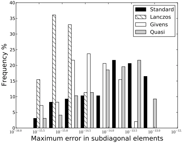
For eachnranging from 1 to 100, we measured the accuracy of reducing the

matrix pair to Hessenberg form by computing the maximum error in the

com-puted subdiagonal entries and the exact subdiagonal entries given in (2.79).

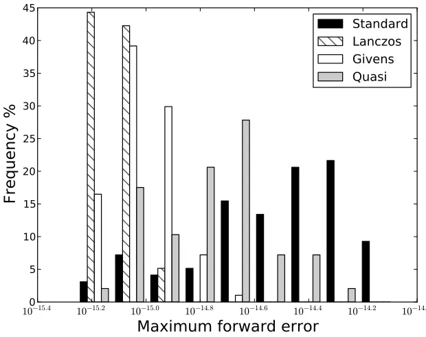
Figure 2.1 reports the maximum error for each value of n. We also measured

the maximum forward error in the computed eigenvalues, as shown in

(49)

Hessenberg-triangular reduction, the Lanczos type reduction of §2.2.1, the Givens type

reduction of§2.2.2, and the quasiseparable matrix algorithm proposed in [6].

10 16.0 ₁₀ 15.5 ₁₀ 15.0 ₁₀ 14.5 ₁₀ 14.0 ₁₀ 13.5 ₁₀ 13.0 ₁₀ 12.5

Maximum error in subdiagonal elements

0 5 10 15 20 25 30 35 40

Frequency %

Standard

Lanczos

Givens

Quasi

Figure 2.1: Distribution of maximum error in the subdiagonal entries of T.

The standard reduction algorithm is not able to make use of the symmetry

of A. This leads to rounding errors propagating into the upper triangular

part ofB. The error in the computed subdiagonal elements of the Hessenberg

matrix and the maximum forward error are the worst of the four algorithms.

The Lanczos type reduction is the most accurate, which was somewhat

surprising given that the transformation matrix could lose orthogonality. It

seems that for this particular set of nodes, the method is fairly well behaved.

Orthogonality of the transformation matrix is lost at a linear rate, that is kQ∗Q−Ik2 ∝n. Forn= 100 we havekQ∗Q−Ik2 ≈10−14. We do not expect

this to be the case for arbitrary sets of nodes. However, it is surprising that

even for equispaced nodes, orthogonality appears to be lost at the same rate.

Eigenvalue Methods for Interpolation Bases

Scholarship@Western

Scholarship@Western

Eigenvalue Methods for Interpolation Bases

Eigenvalue Methods for Interpolation Bases

Eigenvalue Methods for Interpolation Bases

(Thesis format: Integrated-Article)

by

Piers William Lawrence

Graduate Program in Applied Mathematics

A thesis submitted in partial fulfillment

of the requirements for the degree of

Doctor of Philosophy

The School of Graduate and Postdoctoral Studies

The University of Western Ontario

London, Ontario, Canada

Abstract

Co-Authorship Statement

Acknowledgements

Contents

List of Tables

List of Figures

List of Algorithms

List of Notation

Chapter 1

Introduction

1.1

Motivation

1.2

Outline

1.3

A Brief Literature Review

Bibliography

Chapter 2

Fast Reduction of Generalized

Companion Matrix Pairs for

Barycentric Lagrange

Interpolants

1

2.1

Introduction

2.2

Fast Reduction to Hessenberg form

2.2.1

Lanczos Based Reduction

2.2.2

Givens Rotation Based Reduction

2.3

Corollaries, Implications, and Discussion

2.3.1

Complex Nodes

2.3.2

Zero Leading Coefficients in the Monomial Basis

2.3.3

Deflation of Infinite Eigenvalues

2.3.4

Connection to the Chebyshev Colleague Matrix

2.3.5

Balancing

2.4

Numerical Experiments

2.4.1

Chebyshev Polynomials of the First Kind

Maximum error in subdiagonal elements

Frequency %

Standard

Lanczos

Givens

Quasi