Essays on Portfolio Optimization, Simulation and Option Pricing

(1)

Electronic Thesis and Dissertation Repository

1-17-2014 12:00 AM

Essays on Portfolio Optimization, Simulation and Option Pricing

Zhibo Jia

The University of Western Ontario

Supervisor John Knight

The University of Western Ontario Graduate Program in Economics

A thesis submitted in partial fulfillment of the requirements for the degree in Doctor of Philosophy

Follow this and additional works at: https://ir.lib.uwo.ca/etd

Part of the Econometrics Commons

Recommended Citation Recommended Citation

Jia, Zhibo, "Essays on Portfolio Optimization, Simulation and Option Pricing" (2014). Electronic Thesis and Dissertation Repository. 1897.

https://ir.lib.uwo.ca/etd/1897

This Dissertation/Thesis is brought to you for free and open access by Scholarship@Western. It has been accepted for inclusion in Electronic Thesis and Dissertation Repository by an authorized administrator of

(2)

SIMULATION AND OPTION PRICING

by

Zhibo Jia

Graduate Program in Economics

SUBMITTED IN PARTIAL FULFILLMENT OF THE REQUIREMENTS FOR THE DEGREE OF

DOCTOR OF PHILOSOPHY

SCHOOL OF GRADUATE AND POSTDOCTORAL STUDIES WESTERN UNIVERSITY

LONDON, CANADA DECEMBER 2013

c

(3)

This thesis consists of three papers which cover the efficient Monte Carlo sim-ulation in option pricing, the application of realized volatility in trading strate-gies and geometrical analysis of a four asset mean variance portfolio optimiza-tion problem. The first paper studies different efficient simulaoptimiza-tion methods to price options with different characters such as moneyness and maturity times. The incomplete market environments are also been considered. The second pa-per uses realized volatility based on high frequency data to improve the volatil-ity trading strategy. The performance is compared with that using the implied volatility. The last paper re-examines the Markowitz’s portfolio optimization problem using a general case. It also extends the problem to four assets, it describes the exact mean variance efficient fronter in the weight space and studies the frontier in the mean variance space. The thesis may serve to help our understanding of how to apply numerical and analytical methods to solve financial problems.

(4)

I am grateful to my supervisor John Knight for his continuous guidance and support. It is also an absolute pleasure to thank all the people who made this thesis possible.

(5)

Abstract ii

Acknowledgements iii

Table of Contents iv

List of Tables vii

List of Figures ix

1 Introduction 1

2 Empirical Performance

of Efficient Monte Carlo Simulations for Option Pricing

in Incomplete Markets 5

2.1 Introduction . . . 5

2.2 Option Pricing . . . 8

2.2.1 Black Scholes Model in complete markets . . . 8

2.2.2 Incomplete Market Models . . . 9

2.2.3 Monte Carlo(MC) Simulation Approach for Option Pricing 14 2.3 Efficient Monte Carlo Simulation Methods . . . 17

2.3.1 Variance Reduction Techniques . . . 17

2.3.2 Quasi-Monte Carlo (QMC) . . . 24

2.4 Data . . . 25

2.4.1 Real Data . . . 25

2.4.2 Simulated Data . . . 26

2.5 Numerical Results . . . 34

2.5.1 Experiment Using Simulation Data . . . 34

2.5.2 Experiment Using Real Data . . . 39

(6)

3 The effects of the Use of Realized Volatility on Volatility Trading

Strategies 56

3.1 Introduction . . . 56

3.2 Option pricing model . . . 61

3.3 Implied volatility and its prediction . . . 64

3.3.1 Implied Volatility Estimation . . . 65

3.3.2 Implied Volatility Regression . . . 66

3.4 Realized volatility and its prediction . . . 67

3.4.1 Realized volatility . . . 67

3.4.2 Realized Volatility Forecast . . . 69

3.4.3 Using the Predicted Volatility to Price the Options . . . 70

3.5 Data . . . 72

3.5.1 Simulation of Stock and Option Price . . . 72

3.6 The volatility trading strategy: Delta Neutral . . . 77

3.7 Conclusion . . . 85

4 Markovitz’s Four Asset Problem, A Geometrical Analysis 100 4.1 Introduction . . . 100

4.2 Markowitz’s Three Asset Problem . . . 101

4.2.1 Remark . . . 105

4.2.2 Efficient Frontier . . . 111

4.3 Markowitz’s Four Asset Problem . . . 113

4.3.1 The Efficient Portfolio . . . 114

4.3.2 Efficient Frontier . . . 128

4.4 Experimental Results . . . 132

4.4.1 Experiment . . . 132

4.4.2 Monte Carlo Simulation . . . 133

4.5 Conclusion . . . 134

4.6 Appendix . . . 135

4.6.1 Minimum Variance Portfolio . . . 135

4.6.2 Efficient Portfolio with Given Expected Return . . . 137

4.6.3 Efficient Portfolio Area Beneath Point c . . . 139

4.6.4 Explicit Expressions for the Portfolio Mean and Variance in Three Asset Problem . . . 139

4.6.5 Explicit Expressions for the Portfolio Mean and Variance in Four Asset Problem . . . 141

(7)

(8)

2.1 Parameters used in simulation data . . . 43

2.2 RMSE of the Estimates (10000 simulation paths) . . . 44

2.3 Standard Errors of the Estimates (10000 simulation paths) . . . . 45

3.1 Parameters values for the Implied Volatility Regression . . . 89

3.2 Estimate result for the HAR model . . . 90

3.3 Mean Squared Errors in Pricing the Options by IV and RV . . . 90

3.4 Pricing the Option . . . 90

3.5 Daily Profits for Delta-Neutral Trading Strategy

(Generate and analysis data with HW model, No Transaction Cost) . . 91

(Generate and analysis data with HW model, 1% Transaction Cost) . . 92

(Generate and analysis data with HW model, 2% Transaction Cost) . . 93

(Generate data with BS model and analysis with HW model, No Trans-action Cost) . . . 94

(Generate data with BS model and analysis with HW model, 1% Trans-action Cost) . . . 95

(9)

action Cost) . . . 96

3.11 Daily Profits for Delta-Neutral Trading Strategy with adjusted RV (Generate and analysis data with HW model, No Transaction Cost) . . 97

3.12 Daily Profits for Delta-Neutral Trading Strategy with adjusted RV (Generate and analysis data with HW model, 1% Transaction Cost) . . 98

3.13 Daily Profits for Delta-Neutral Trading Strategy with adjusted RV (Generate and analysis data with HW model, 2% Transaction Cost) . . 99

4.1 . . . 132

4.2 . . . 133

4.3 . . . 133

4.4 . . . 134

(10)

2.1 RMSE of Estimates based on generated data by SV model . . . . 46

2.2 RMSE of Estimates based on generated data by Jump model . . . 47

2.3 RMSE of Estimates based on generated data by SVCJ model . . . 48

2.4 SE of Estimates based on generated data by SV model . . . 49

2.5 SE of Estimates based on generated data by Jump model . . . 50

2.6 SE of Estimates based on generated data by SVCJ model . . . 51

2.7 SE by Simulation Number of Samples on Call Option of S&P500 52 2.8 SE by Time on Call Option of S&P500 . . . 53

2.9 RMSE by Simulation Number of Samples on Call Option of S&P500 54 2.10 RMSE by Time on Call Option of S&P500 . . . 55

3.1 Five paths of simulated stock prices for one year . . . 88

3.2 One simulation of call option and put option prices for one year . 89 4.1 . . . 103

4.2 . . . 107

4.3 . . . 109

4.4 . . . 111

4.5 . . . 112

4.6 . . . 114

4.7 . . . 118

4.8 . . . 119

4.9 . . . 123

(11)

4.12 . . . 129

(12)

Chapter 1 Introduction

The dissertation consists of three papers dealing with efficient Monte Carlo simulation strategies for option pricing, the use of realized volatility in high fre-quency volatility trading strategies and a geometrical analysis of Markovitz’s four asset problem.

(13)

Variables, Control Variates, Stratified Sampling (SS), Importance Sampling, and Quasi-Monte Carlo (QMC). The comparison was made on different money-ness and maturity times. According to Root Mean Squared Error, QMC is the best choice for the out-of-the-money options. For in-the-money options, there was no clear winners as the performance of the methods changed with the op-tion pricing model. Considering the standard error, QMC and SS did the best and much better than the other methods. The study may serve to improve the speed and accuracy of Monte Carlo methods for option pricing under incom-plete environments.

(14)

that of implied volatility, and this would be important in practice because the application of the realized volatility improves the calculation efficiency.

(15)

(16)

Chapter 2 Empirical Performance

of Efficient Monte Carlo

Simulations for Option Pricing

in Incomplete Markets

2.1 Introduction

The benchmark model for option pricing is the Black-Scholes(B-S) model, which assumes that the market is complete. For instance, an investor can borrow as much as he needs at a constant risk-free interest rate; there is no transaction cost in the market; the underlying asset prices follow the Geometric Brownian Motion(GBM) process with constant drift and volatility; it is free of short sell-ing constraints in the market, etc. The B-S model uses no-arbitrage theory and martingale methods to get a closed form of option price in the complete market.

(17)

it can bring out the main features of the option price. However, it has been crit-icized for its normal distribution and the complete market assumptions. For example, the empirical data show conflicts in this model, such as leptokurosis with the assets return having a higher peak and heavier tails than the normal distribution; the ”smile” in volatility can not be explained by the Black-Scholes model. Also, the volatility of the underlying asset return can not maintain con-stancy. The Black-Scholes option pricing model comes from replicating portfo-lios to cover the risk totally. However, it needs to be recognized that the market is significantly incomplete and the perfect replication is impossible. There are many factors contributing to the incompleteness of the market. Factors such as transaction costs, portfolio constraints, insufficient assets for investing and the volatility in B-S model can not be perfectly estimated. In this paper, the models used to describe the incompleteness are stochastic volatility and mixed jump diffusion processes which can better match the empirical data than in B-S model.

(18)

advantages compared to other numerical methods. It is easy to apply to com-plicated problems, and with it people can simulate the paths and estimate the expectations in most cases. The convergence speed does not rely on the dimen-sion number of the problem. Moreover, the Monte Carlo estimate can provide more accurate confidence intervals.

In order to get more accurate results with the Monte Carlo simulation method, a large number of replications are needed. Thus, efficient strategies are almost compulsory in order to reduce the variance of the estimator and improve the accuracy. The popular variance techniques include antithetic variates, control variates, moment matching, stratificaiton and Latin hypercube sampling, im-portance sampling, repricing-matching-weights, conditional Monte Carlo and Quasi-Monte Carlo simulation.

Much research has been done in the field of applying Monte Carlo simulation to pricing the American style option and path dependent option, such as Asian options. However, how to apply the efficient simulation in the environment of incomplete market has not drawn much attention. The goal of this paper is to apply and compare the various efficient simulation strategies in pricing the European style options in the incomplete financial markets.

(19)

option pricing models in the incomplete markets and the Monte Carlo method to price options. Section 2.3 presents the efficient simulation methods such as four variance reduction techniques and Quasi-Monte Carlo method. Section

2.4describes the data used in this research including generated data and real data. Section 2.5 provides the numerical results and Section2.6draws conclu-sions.

2.2 Option Pricing

2.2.1 Black Scholes Model in complete markets

It is assumed that the stock prices follow a (continuous time) geometric Brow-nian motion process:

dS =φSdt+σSdW (2.1)

where,

S = the current stock price

φ = the expected return

σ = volatility of the stock return

W = Brownian Motion process

dW = (dt)0.5, is the standard normal distributed random variable

(20)

it is possible to borrow and lend cash at the risk-free interest rate, the Black-Scholes European call option price can be obtained as:

fBS = SN(d1)−Ke−rTN(d2) (2.2)

Where,

S = current stock price

K = option strike price

r = annual risk-free interest rate

T = time to expiration, current time is set to zero, T should be annualized since the annual interest rate is used

N = the cumulative normal density function

d1 =

ln(S/K) + (r+σ2_/₂₎_T

σT1/2

d2 =

ln(S/K) + (r−σ2/2)T

σT1/2 =d1−σT 1/2

2.2.2 Incomplete Market Models

(21)

Stochastic Volatility Model (SV)

In the incomplete market, the underlying asset return volatility is stochastic rather than constant. We use the Hull and White (1987) model to describe the option prices process. If the stock price is St and its instantaneous variance is Vt, the asset price can be described in the following stochastic processes,

dS =S(φdt+σdw) (2.3)

dV =V(µdt+ξdz) (2.4)

Where V =σ2 _{follows a geometric Brownian Motion.} _dw _and _dz _{are correlated}

Brownian motion process with correlation coefficient ρ. φ is the expected re-turn of the share, µis the drift (expected growth rate) of the variance,σ is the volatility andξis the volatility of volatility. The security pricef(St, σ2t, t)is the

present value of the expected terminal value of f discounted at the risk free rate, thus the closed form of the option price is:

f(St, σt2, t) =e −r(T−t)

Z

f(ST, σ2T, T)p(ST|St, σt2)dST (2.5)

WhereT is the time at which the option matures,Stis the security price at time

t, σt is the instantaneous standard deviation at time t, and p(ST|St, σt) is the

conditional density function ofST given the security price and variance at time

t. V = _T1₋_tR_tT σ_τ2dτ denotes the mean of variance over the life of the derivation security, and the price can be written as

f(St, σt2, t) = Z

e−r(T−t) Z

f(ST)g(ST|V)dST

h(V|σ2

(22)

where h(·) denotes the conditional distribution of V. The inner integral pro-duces the Black-Scholes price.

If we assume that the correlationρ= 0andµandξare independent ofS(t), the Hull and White price can be seen as the integral of the Black-Scholes price over the conditional distribution of mean variance V and in Hull and White(1987) model:

fHW(St, σt2) = Z

fBS(V)h(V|σ2

t)dV (2.7)

fBS _{is the Black-Scholes European option price defined in previous section.}

By expanding Black-Scholes price fBS₍_V₎ _{from its expected average variance} E(V)in a Taylor series, Hull-White also propose a power series approximation technique to get the option pricefHW _as:

fHW(St, σt2) = f

BS₍_E₍_V_{)) +} 1

2

∂2_fBS₍_E₍_V₎₎ ∂V2

E(V2)

+1 6

∂3_fBS₍_E₍_V₎₎ ∂V3

E(V3) +... (2.8)

WhereE(V2)and E(V3)are the second and third central moments ofV.

Jump-Diffusion Model(Jump)

(23)

Brownian motion as in Black-Scholes(1973) model, together with jumps which are modeled with a compound Poisson process. The dynamics of the stock prices is described as

dS/S = (φ−λµ)dt+ ˆσdWt+dqt (2.9)

Whereφ is the instantaneous expected return of the asset,λis the mean num-ber of arrival events in unit time, µ is the mean jump size. σˆ2 _{is the}

instan-taneous variance of the return when the Poisson event does not occur. Wt is

a standard Brownian motion. qt is the independent Poisson process. And the

price of an European call option in Jump-Diffusion model is given by

fJ =

∞ X

i=0

e−λT₍_λT₎i i! f

BS₍_{S, K, T, r, σ}

i) (2.10)

where T is the time to expiration; K is the strike price; r is the annual risk free interest rate; fBS₍_{S, K, T, r, λ}

i)is the Black-Scholes pricing formula for an

European Call option, and

σi = p

z2₊_δ2₍_i/T₎_,

where

z2 =σ2−λδ2, δ2 = γσ

2

λ

(24)

Stochastic Volatility with Concurrent Jumps in the Stock Price and

the Variance Process(SVCJ)

There is strong empirical evidence of stochastic volatility and jumps in finan-cial markets. We follow the SVCJ model in Duffie et al.(2000) which is based on the dynamics of the underlying stock price and variance,

dSt = (φ−λµ)Stdt+ p

VtSt h

ρdW_t(1)+p1−ρ2_dW(2)

t i

(2.11)

+(Js−1)dNt

dVt = k(θ−Vt)dt+σv p

VtdW

(1)

t +J v_dN

t (2.12)

whereStis the stock price at timet,φ is the interest rate, √

Vtis the volatility, θ is the long-run mean of variance, k is the speed of mean reversion, σv

de-termines the volatility of the variance process,W_t(1) and W_t(2) are independent Brownian motion processes, andρis the instantaneous correlation between the return process and the volatility process.

Nt denotes a Poisson process independent of the Brownian motions with

con-stant intensity λ, Js _{is the relative jump size of the stock price and} _Jv _{is the}

jump size of the variance. If a jump occurs at timet, we have

S_t+ =S_t−Js

Vt+ =V_t−Jv

(25)

µvandJsfollows lognormal distribution with mean(µs+ρJJv)and varianceσs2.

And the parameters µs andµare related as µs =log[(1 +µ)(1−ρJµv)]−0.5σs2.

There is no closed form solution for the option price in SVCJ model and it only has numerical solution.

2.2.3 Monte Carlo(MC) Simulation Approach for Option

Pricing

The Monte Carlo simulation method was first used in option pricing by Boyle and it has proved to be a powerful tool in finance. There has been a lot of research on the MC simulation in American style options and path depended options such as Asian options, but not much attention has been given to the incomplete market environment. There is a lot of work to do on the improve-ment of the algorithm of MC approach in this field. This paper focuses on how to choose the efficient strategies of MC simulation in the incomplete market environment. Following is the basic MC approach which simulates the process of how an option is priced.

The payoff for an European call option with strike price K at expiry time T

isfcall(S, T, K) = max{ST −K,0}whereST is the point stock price. Monte Carlo

(26)

for each path and takes average to get

¯

fcall(S, T, K) =

1

m m X

i=1

f_call(i)(S, T, K) (2.13)

The approximation of the present time option price is obtained by discounting the approximate future price bye−rT_{, where}_r _{is the risk free interest rate.}

ff air(S,0, K) = e−rTf¯call(S, T, K) (2.14)

Following one of the assumptions of Black-Scholes model, we simulate the un-derlying stock prices whose natural logarithm follow a geometric Brownian motion process. Same as equation (2.1), the stock prices dynamic is described as the SDE:

dS =φSdt+σSdW (2.15)

By Ito’s Lemma,

ST =Stexp{(φ−0.5σ2)(T −t) +σ √

T −t} (2.16)

This is the continuous time model of the underlying stock price at maturity time T. Accepting the risk neural assumption, stock return φ is equal to the risk-free interest rate rf. However, φ can also denote the cost of carry rate

which is the cost of interest plus additional costs such as the cost of paying dividends.

(27)

minutes. In order to simulate the stock prices, we separate 1 year into n pe-riods. Assuming that there are N days in a year and Dperiods every day, we have n = N ∗D and the maturity time T(days) is scaled to T∗ = T ∗D peri-ods. The asset return per period isφ∗ = φyear

n . The asset volatility per period is σ∗ = σ_√year

n . The stock prices process follows lognormal distribution. If current

time ist = 0, stock price at scaled maturityT∗ is:

S(T∗) =S(0)exp{ T∗ X

i=1

Zi} (2.17)

whereZi follows the normal distribution with meanµ=φ∗−1₂(σ∗)2 and

volatil-ityσ∗. Equation (2.17) can also be written as

S(T∗) = S(0)exp{µT∗+σ∗√T∗

i} (2.18)

i is drawn from a standard normal distribution. If we have simulated the

stock price at maturity, the present-time fair option price can be obtained by discounting the payoff to the factore−rT _as

f(S0) =

1

me −rT

m X

i=1

[max{ST −K,0}] (2.19)

The number of replications m must be set large enough, such as 104_{, to get}

(28)

2.3 Efficient Monte Carlo Simulation Methods

2.3.1 Variance Reduction Techniques

The convergence speed of Monte Carlo simulation isN−12, but there are several

variance reduction methods which can improve the accuracy of the simulation process. I use four techniques in this paper to compare their performance in the incomplete market.

Antithetic Variables(Anti-V)

Anti-V uses pairs of random variables that follow the same probability dis-tribution but with negative correlation. The average of N pairs of antithetic variables has smaller variance than that of 2N independent variables. If we want to estimate E(h(U)) whereU is uniformly distributed on [0,1]N_{. We can}

get the antithetic variate ofU,

1−U= (1−U1,1−U2, ...,1−UN)

Now we can estimatehby

¯

h= 1

N N X

i=1

h(Ui)

and

¯

hA= 1

N N X

i=1

h(1−Ui)

The Antithetic estimator is(¯h+ ¯hA)/2. The variance of this estimator is

V ar(h(U))

(29)

whereρis the correlation betweenh(U1)andh(U1A). The variance is reduced if

ρ <0, and it is always the case ifV ar(h(U))is monotonic inU. The idea is that

hcan be decomposed to symmetric part(h(U) +h(1−U))/2and antisymmetric part (h(U)−h(1−U))/2. Because the Antithetic version of estimator has only the symmetric part ofh, the variance is reduced.

In this study, option prices are simulated based on normal random variable

Zi and−Zi. Option prices are

fi = e−rTmax{0, S

(i)

T −K}, whereS

(i)

T is simulated based onZi (2.20)

˜

fi = e−rTmax{0,S˜

(i)

T −K}, whereS˜

(i)

T is simulated based on−Zi (2.21)

and an unbiased estimator of the option price is

fAntiV =

1

N N X

i=1

fi+ ˜fi

2 (2.22)

Control Variates(CV)

The control variates method adjusts the outputs of Monte Carlo simulation directly. It uses the known errors of the estimator which contains the infor-mation of the unknown error of the interesting estimator, for example, in the case of estimatingE(h(X))orE(h(X1, ..., XT)). Suppose we knowE(f(X))and

(30)

Now let

¯

h = 1

N N X

i=1

h(Xi)

¯

f = 1

N N X

i=1

f(Xi)

σ2_h = V ar(h(X))

σ_f2 = V ar(f(X))

Construct new estimator

¯

hα = ¯h+α(E(f(X))−f)

Since E(¯hα) = E(h(X)), the new estimator is still unbiased. However, the

variance for the new estimator is

V ar(¯hα) =

1

N(σ

2

h+ 2ασhσfρ(h(X), f(X)))

Given the variances and correlation, it is obvious that

ˆ

α =argminαV ar(¯hα) = −(σh/σf)ρ(h(X), f(X))

andminα =σh2(1−ρ

2₎_/N_{. The more}_h₍_X₎_and_f₍_X₎_{are correlated, the more the}

variance is reduced.

(31)

price andc=E[C]wherecis the true value of the option. We letST be the

sim-ulated terminal price of the underlying stock at time T. By the Black-Scholes assumption, we have the expected value of terminal asset price E[ST] = S0erT.

Now we can construct a control variates estimator of the option price as

CCV =C+α(erTS0−ST) (2.23)

since the variance of the new estimator is

V ar[CCV] =V ar[C] +α2V ar[ST]−2αCov[C, ST] (2.24)

αis chosen to minimizeE[CCV ₋_c_]2 _{and the variance-minimizing}_α _is

α∗ = Cov(C, ST)

V ar(ST)

(2.25)

This problem can be solved by a linear regression ofC onST.

Stratified sampling(SS)

Random variablesXi are sampled in a way that a specified number of samples

selected from each stratum. Thus, the whole domain can be covered. It is useful if there is a good approximation for the average over small subdomain. The stratification should be chosen so that the subdomains have equal probability associated. Considerh(U1, ..., Ud), the standard stratified sampling is to divide

the sample space of U1 into equiprobable strata [0,1/N], ...,[(N −1)/N,1] and

the stratified estimator can be described as

1

N N X

i=1

h i−1 +U

(i) 1

N , U

(i) 2 , ..., U

(i)

d !

(32)

Note that(i−1 +U₁(i))/N falls between(i−1)th and ith with probability1/N.

In general, if we want to sample from a mix of N distributions in which the

ith distribution has probability pi, mean µi and variance σi2. Thus, the mixed

distribution has mean

N X

i=1

piµi

and variance

N X

i=1

pi(µ2i +σ

2

i)− N X

i=1

piµi !2

Applying the stratified sampliing, the variance of the new stratified estimate isPN_i₌₁piσi2, and the variance reduction is

N X

i=1

pi(µ2i)− N X

i=1

piµi !2

The SS removes the variance of conditional expectation of the outcome given the information being stratified.

In our option pricing case, the payoff depends mainly on the terminal stock priceST which is assumed to follow a Brownian motion processW. If we want

to generate 105 _{times standard normal distributed number, we can apply SS}

process to improve the simulation. For example, separate the whole field to103

straddles and do 102 _{independent simulations in each straddle. The random}

number in each straddle is

z_ij = Φ−1

i−1 +Ui

103

(33)

Where Φ−1 _{is the inverse cumulative distribution function of a standard}

nor-mal,Ui is drawn fromU nif(0,1). Then in theithstraddle, we simulate random

number z_ij 102 _{times. Note that} i−1+Ui

103 falls between the (i−1)th and ith

per-centiles of the uniform distribution with equally probability.

Importance sampling (IS)

In Monte Carlo simulation process, importance sampling is applied to change the measure for obtaining a new estimator with lower variance. Random vari-ables Xi’s are selected according to a different probability measure Q. The

probability measure Qis viewed as a way to control the choice ofXi’s in order

to consider the underlying structure of value functionh. We use the likelihood ratioswi’s to remove the bias due to sampling from measure Q. It also can be

viewed as an indirect way to bias the sampling towards the ”important” sam-ples. In finance, importance sampling is mostly used to ensure that all samples are drawn in the regions where the function is nonzero, for example, pricing the out-of-money option. The standard process of generating paths will lead to many zero payoffs. The idea of using IS as variance reduction technique is that the estimate under new measure has less variance than that under the initial probability measure. For example, if the payoff hcan be obtained by simulat-ing many paths of X1, ...., Xm and take average. This process is the same as to

estimate the integral

Z

h(x)g(x)dx=

Z

hg

˜

g

(34)

where ˜g is nonzero. Now the payoff is ˜h = hg_g_˜ under new measure. The im-portance sampling method chooses ˜g such that the payoff ˜h has less variance under the new measure. The ideal way is to choose g˜ = hg_µ to make the new payoff have zero variance. But constant µ = R

h(x)g(x)dx is unknown. Thus the goal of importance sampling is to choose density˜g proportional tohg.

The ideal importance sampling can construct a zero-variance estimator by sam-plingST from the density,

f(x) =c−1max{x−K,0}e−rT_g₍_x₎ _(2.29)

whereg()is the log-normal density ofST;cis a constant which normalizes the

integration of density function f to 1. Here, c is just the current time option price. It is not applicable in practice.

Following Boyle(1997), we apply importance sampling in pricing the European style call option. We need to price the option by e−rT_E_[_max{S

T −K,0}]. The

standard approach is to generate samples of the terminal prices ST in (2.16)

with Brownian Motion having drift r and volatility σ. However, we can also generate ST with any other drift µand adjust the expectation with the

likeli-hood ratio. We use higher drift in importance sampling to obtain higher per-centage of sample paths with positive payoffs.

(35)

where L is the likelihood ratio of the log-normal densities with parameters µ

andr defined as

L=

ST S0

(r−µ)/σ2 exp

(µ2₋_r2₎_T

2σ2

(2.31)

2.3.2 Quasi-Monte Carlo (QMC)

Quasi-Monte Carlo simulation, which uses the Low-discrepancy sequences and is also called Quasi-random sequences, can provide a convergence ofO(N−1₍_log₍_N₎₎d₎_,

wheredis the dimension number of the integration. The standard Monte Carlo offers convergence as O(1/√N). Thus, QMC sequence improves the conver-gence when the dimension d is small. QMC uses pre-selected deterministic points rather than random samplings to evaluate the integral. The accuracy of this approach depends on how the deterministic points are dispersed through-out the domain of integration.

There are two main approaches to construct QMC which are randomized QMC (RQMC) and effective dimension. We use the RQMC based on Lemieux and L’Ecuyer(2001). First, we use lattice rules, Korobov rules specifically, to create the low-discrepancy point set. For sample size n and dimension d, we choose an integer a ∈ {1, ..., n−1} and letaj =aj−1 mod n , f or j = 1, ..., d. The lattice point setPn ind dimensions is described as

Pn ={ i

n(1, a, a

(36)

Second, get the randomize QMC point sets. We randomly generate a vector∆

in[0,1]d_{and add it to each point of}_P

n with modulo 1. i.e. RQMC point setP˜nis

˜

Pn= (Pn+ ∆)mod1 (2.33)

To apply QMC in estimating the call option price, we take Ui’s from RQMC

sequence rather than from the uniformly distributed variables in MC sequence.

2.4 Data

2.4.1 Real Data

For the real data, we use the European type call options on the S&P 500 in-dex(SPX) because this is one of the most actively traded options in the world. The daily dividend distributions of the index are available. Furthermore, there has been a lot of research based on the SPX.

(37)

days). The options are also classified as in-the-money(K/S ≤ 0.97); at-the-money(K/S ∈(0.97,1.03)) and out-the-money(K/S≥1.03).

2.4.2 Simulated Data

It is useful to test the efficient simulation strategies on the simulated data since we will be able to examine their performances under exact models. We use the SV, Jump-diffusion and SVCJ models in this study. In the SV model and Jump-diffusion model, closed form option prices are taken as ”true” price. There is no closed form price for SVCJ model and I use the almost exact simu-lation methods discussed in Alexander & Antoon (2008) to generate the ”true” price.

(38)

only simulate 180 days to compare with the short term options. Strike stock ratios are 0.8 as in-the-money, 1.0 as at-the-money and 1.2 as out-of-the-money in this study.

Option Price in Stochastic Volatility(SV) model

In SV model, we use the option price form of Hull and White (1987) in equation (2.8) in which the Black-Scholes price is obtained from equation (2.2). The result depends on the parameters µ and ξ. Assuming µ is zero and by the moments for the distribution ofV, the Hull-White option price can be described as:

fHW(S, σ2) = fBS(σ2)

+ 1 2

S√T −tN0(d1)(d1d2−1)

4σ3 ×

2σ4₍_ek₋_k₋₁₎

k2 −σ

4

+ 1 6

S√T −tN0(d1)[(d1d2−3)(d1d2−1)−(d21+d22)]

8σ5 (2.34)

× σ6

e3k₋_{(9 + 18}_k₎_ek_{+ (8 + 24}_k_{+ 18}_k2_{+ 6}_k3₎

3k3

+...,

where fBS₍_σ2₎ _{is the Black-Scholes price and} _σ2 ₌ _E_{[ ¯}_V_{] =} _V

0. k = ξ2(T −t)

which is sufficiently small and ξ is from 1 to 4. From Hull and White(1987),

ξ = 1 leads to the least bias when pricing the options with stochastic volatili-ties.

(39)

dynamics in Hull-White model, Monte Carlo simulation can be used to get the numerical solution according to the following equations:

Si = Si−1exp{(φ−

Vi−1

2 )∆t+ui

p

Vi−1∆t} (2.35)

Vi = Vi−1exp{(µ−

ξ2

2)∆t+viξ

√

∆t} (2.36)

The annualized interest rate φ is set to 0.07 and µ is set to 0. i is the index where1≤i≤n. ui and vi are sampled from independent standard normal

dis-tributions. V0 can be obtained fromV0 =σ20 whereσ0 is obtained from the S&P

500 index option. In Hull and White (1987) model, the correlation ρ between stock price and variance is assumed to be zero to get closed form option price. I keep the assumption here.

In order to simulate one year’s daily option prices, we need to simulate the stock prices first. The time interval t∗ −t = 1 is separated to n subintervals and ∆t = (t∗−t)/n wheret is set to zero. I simulate 96 observations each day and apply the last one in the Black-Scholes formula to obtain the option price of that day. In this case,n = 96∗250. The stock prices are taken to calculate the daily option prices are at index i = 96h, where h is the date number. When I have the closing time stock price for dayh, the Hull-White option pricef_hHW is obtained from equation (2.34). Replicating this processmtimes independently, and the simulated option price at dayhis described as

fHW_h = 1

m j=1

X

m

f_hHW (2.37)

(40)

Option Price in Jump-diffusion model

Jump-diffusion model has closed form for option price as described equation (2.10). In order to sum from0to∞in the price equation, a stopping rule is set for the iteration.

Simulated Option Price in SVCJ model

Although Broadie and Kaya(2006) have given an exact simulation for the SV model, the process is slow and can barely be used in practice. In this study, I use the direct interpolation combined with the Quadratic Exponential scheme in Andersen(2007) and martingale correction in Andersen and Piterbbarg (2007) to obtain an efficient simulation process.

At timet, givenSu andVu, foru < t, the dynamics of stock priceStand variance Vt are described as

St = Suexp[(φ−λµ)(t−u)−0.5 Z t

u Vsds

+ρ Z t

u p

VsdWs(1)+ p

1−ρ2

Z t

u p

VsdWs(2)] (2.38)

× Nt

Y

i=Nu+1

J_is

and the variance is

Vt = Vu+kθ(t−u)−k Z t

u

Vsds+σv Z t

u p

VsdWs(1)

+

Nt

Y

i=Nu+1

(41)

In this study, we follow the option price simulation algorithm in Broadie and Kaya(2006), but use the alternative efficient simulation rather than the exact simulation in the second step. The time horizon is divided according to the jumps and the variance, and stock prices are simulated at each jump. The algorithm for simulation option price based on SVCJ model is described as fol-lowings:

Step 1

Simulate a Poisson process with intensity λ to determine the time for the jumps. If the maturity is T, the expected jump times during this time hori-zon isλ∗T. Also, the time of next jumptj is set toT iftj > T. For the property

of a Poisson process, time between two jumps Rj has an exponential

distribu-tionExp(λ)with mean 1

λ. The steps to simulate the jump timetj are described

as followings

1 , generateRj from exponential distributionExp(λ), i.e.E(Rj) =

1

λ

2 , tj =tj−1+Rj

Step 2

During the time interval tj −t0, we ignore the jump process and simulate the

stock priceStj and varianceVtj according to the SV model. The time grid is set

(42)

WhereM = tj−t0

∆t and∆t = 5minutes. The stock price and variance process are dSt

St

= φdt+√vtdWts (2.40) dvt = k(θ−vt)dt+σv

√

vtdWtv (2.41)

wheredW_tsdW_tv =ρdt. The exact solution of (2.40) is

St=Ssexp Z t

s

[φ−0.5vu]du+ Z t

s √

vudWus

(2.42)

Using Ito’s Lemma and Cholesky decomposition, we have

log(St) = log(Ss)−0.5 Z t

s

vudu+ρ Z t

s √

vudWuv

+p1−ρ2

Z t

s √

vudWu (2.43)

By integrating the variance process (2.41), the variance can be described as

vt = vs+ Z t

s

k(θ−vu)du+σv Z t

s √

vudWuv (2.44) or

Z t

s √

vudWuv =

1

σv

vt−vs−kθ∆t+k Z t

s vudu

(2.45)

Plugging (2.45) into (2.43), the logarithmic asset price is

log(St) = log(Ss) + kρ σv

Z t

s

vudu−0.5 Z t

s

vudu+ ρ σv

(vt−vs−kθ∆t)

+ p1−ρ2

Z t

s √

vudWu (2.46)

Drift interpolation

The simple drift interpolation scheme is defined as

Z t

s

(43)

Applying the drift interpolation into equation (2.46), we have the approximate logarithmic stock price as

log(St) =log(Ss) +φ∆t+K0+K1vs+K2vt+ p

K3vs+K4vtZs (2.48)

whereZsis drawn from a standard normal distribution, and

K0 = −

ρkθ σv

∆t, K1 =γ1∆t

kρ σv

−0.5

− ρ

σv

, K2 =γ2∆t

kρ σv

−0.5

+ ρ

σv

K3 = γ1∆t(1−ρ2), K4 =γ2∆t(1−ρ2)

Quadratic Exponential(QE) Scheme for Variance Process

Givenvs, compute

m = θ+ (vs−θ)e−k∆t

s2 = vsσ

2

ve−k∆t k (1−e

−k∆t_{) +} θσ

2

v

2k (1−e −k∆t₎2

ψ = m

2

s2

Letψc = 1.5. (a) Ifψ ≤ψc,

b2 = 2ψ−1−1 +p2ψ−1p₂_ψ−1 ₋₁

a = m

1 +b2

vt = a(b+Zv)2

whereZv is drawn from a standard normal distribution. (b) Ifψ > ψc,

p = ψ−1

ψ+ 1

β = 1−p

m =

2

m(ψ + 1)

(44)

whereUv is drawn from an uniform distribution andL−1 is defined as

L−1(u) =

(

0 0≤u≤p

β−1log(₁1₋−_up) p≤u≤1

Martingale Correction

Since the discretized stock price from equation (2.48) does not satisfy the mar-tingale condition under the risk-neutral measure, we apply the marmar-tingale cor-rection scheme in Anderson(2007) in the QE process. The method is to replace

K0 in equation (2.48) by modified parameterK0∗ which is described as

K₀∗ =

(

− Ab2_a

1−2Aa + 0.5log(1−2Aa)−(K1+ 0.5K3)vs ψ ≤ψc −log(p+ β_β(1₋−_Ap))−(K1+ 0.5K3)vs ψ > ψc

whereA=K2+ 0.5K4.

Simulation Algorithm

Givenv0,ψc= 1.5,γ1 =γ2 = 0.5,

1, Use QE scheme to samplevt.

2, Calculate the parameterK₀∗ using the martingale correction method. 3, Generate the stock priceStfrom equation (2.48).

Step 3

If the next jump timetj is equal or larger than T, this jump is skipped and the

stock price at maturity isST. Otherwise, we simulate the jumpξv for volatility

at time tj. The jump size is sampled from exponential distribution with mean µv. The variance when jump occurs is updated asV˜tj =Vtj +ξ

(45)

Step 4

The jump of stock priceξs _{is also simulated at time}_t

j. The jump sizeξsis

sam-pled from a lognormal distribution with mean µs+ρJξv and variance σs2. The

stock price at jump is set toS˜tj =Stjξ

s_.

Step 5

Now the new stock price and variance are updated asS0 = ˜Stj, V0 = ˜Vtj, t0 =tj,

and repeat fromstep 1to get next jump until we reach the maturity timeT.

The payoff of the option is simulated by taking average on enough number of paths and discount to the factore−rT _{to get present-time fair option price.}

2.5 Numerical Results

2.5.1 Experiment Using Simulation Data

(46)

experiments.

For each option price model(SV, Jump, SVCJ), we do the experiment 500 times. In each experiment, one year’s daily option prices are simulated according to specific model and are taken as the ’true’ prices. Monte Carlo with different efficient simulation strategies is used to estimate the option price for every-day. The simulations number in each experiment is from 500 to 5000. The estimated price is compared with the ’true’ price. We use the standard error and the root mean squared error to measure the accuracy. Each Monte Carlo simulation takes replications number m, which is important for the accuracy. In each experiment we change the values ofmand change the expiration time and moneyness. The standard error of the mean(SE) and Root Mean square error(RMSE) are defined as

SE = √s

N,wheres= v u u t

1

N−1

N X

i=1

(fi−f¯i)2 (2.49)

RM SE =

s PN

i=1(fi−fi∗)2

N (2.50)

where

s the sample standard deviation

N the sample size

fi option prices obtained by MC simulation

¯

fi average of option prices obtained by MC simulation

(47)

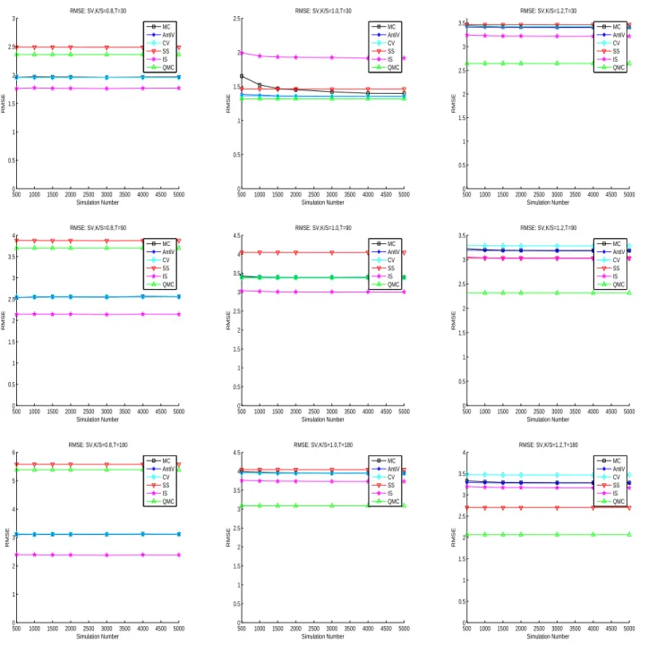
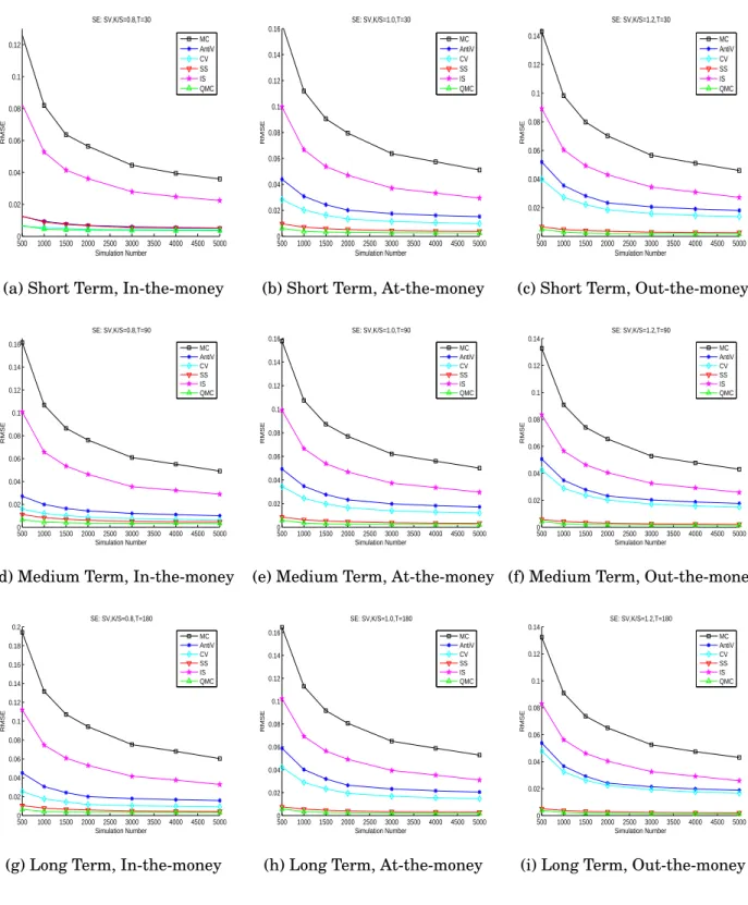
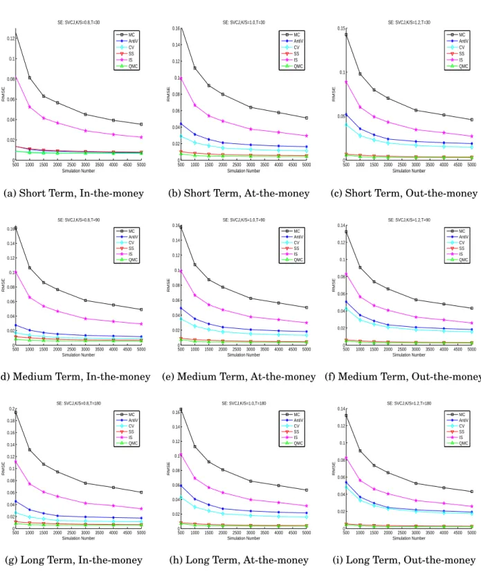
The standard error(SE) measures the standard deviation of the estimates’ sam-pling distribution. The root mean squared error (RMSE) defined in this re-search measures the distance between the estimated prices and the true prices. The results of RMSE are in Table 2.2 and Figure 2.1 to Figure 2.3. The results of standard errors are in Table 2.3 and Figure 2.4 to 2.6. From the numerical results, we can have some interesting findings as follows:

For the results of the RMSE, it is clear that the the effects are different based on different option pricing models, strike stock ratios, and maturity times.

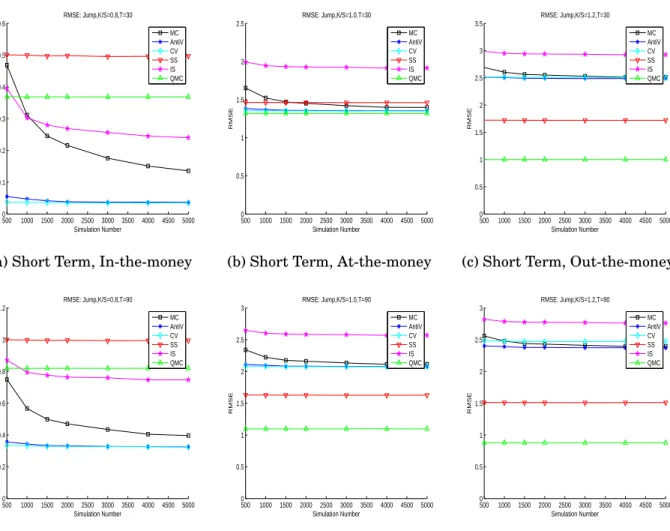
Firstly, the results under option pricing models are: For SV model, IS

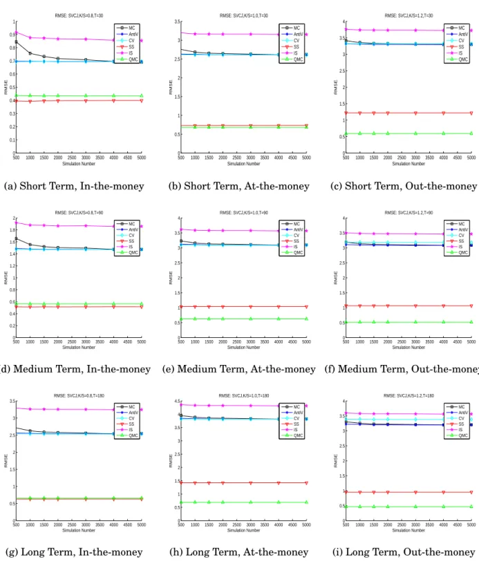
per-forms the best for in-the-money option and QMC perper-forms the best for most cases in at-the-money options and out-the-money options. For Jump model, CV performs the best for in-the-money option, but QMC does the best for the at-the-money options and out-at-the-money options. For SVCJ model, SS does the best for in-the-money option and QMC performs the best for the at-the-money and out-the-money options.

Secondly, the results based on times to maturity are: For the short term

(48)

the medium term options(90 days), QMC does the best in at-the-money option and out-the-money options. The other different methods perform the best for in-the-money options. It is the same for long term options(180 days); QMC does the best for at-the-money and out-the-money options, while the other methods beat QMC for the in-the-money options.

Thirdly, considering the strike stock ratios, different models and maturity

times show different results. For in-the-money options, IS performs the best for all maturity times in SV model. CV and AntiV both do the best in the Jump model. SS and QMC both do the best in the SVCJ model. For at-the-money options, QMC does the best in most cases except that IS does the best for the medium term option based on SV model. Also SS and AntiV work as well as QMC does in in-the-money options. For out-the-money options, QMC does the best and much better than the other methods. SS also performs better than the other methods except QMC method.

(49)

and offer better results in this case. The reason may be that, we only chose the simplest algorithm in this study rather than the complex time consuming optimal algorithm. Also, in some cases, not all the efficient simulations can produce better results than the standard Monte Carlo; some even performed worse.The accuracy doesn’t improve significantly with increasing the simula-tions number. RMSE measures the distance between the true option prices and the prices obtained by Monte Carlo simulation. It is even more important in practice than the standard error. In order to get more accurate prices in the incomplete market, we should choose right efficient simulation strategies and better pricing algorithms as well.

(50)

2.5.2 Experiment Using Real Data

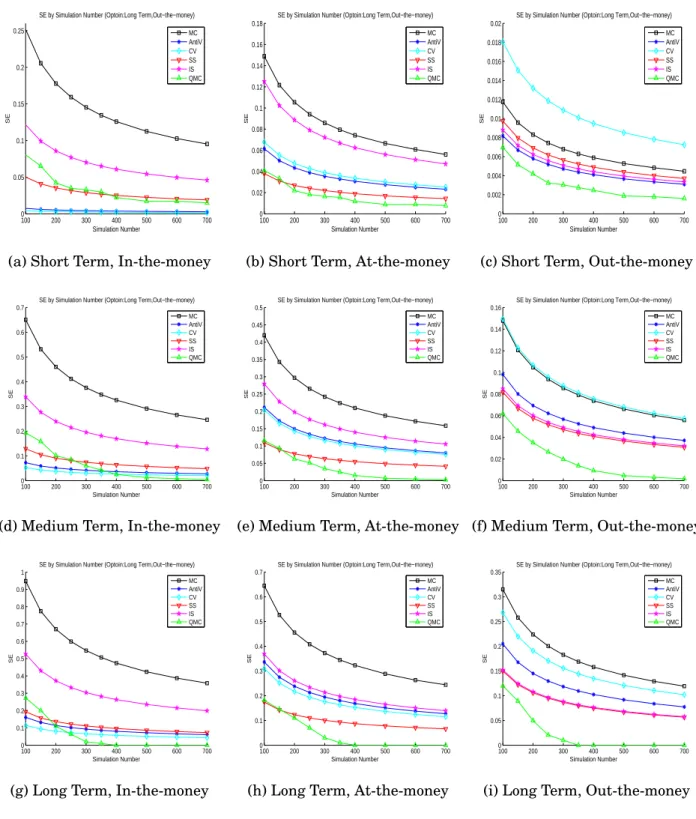
In this research, we use the European style call options on S&P 500 index of a specific day. The options are filtered and categorized as described in section

2.4.1. We compared the standard error (SE) and the root mean squared error (RMSE) based on different simulation times. The SE and RMSE based on CPU time in seconds used in simulation are also counted and compared. The exper-iment results are close to that based on the generated data from models but different to some extent. Experiments results are listed in Figure2.7, 2.8, 2.9

and2.10.

According to standard error of simulations on the in-the-money options, all efficient methods do much better than the standard Monte Carlo simulation. The stratified sampling and Control variate did the best, and the quasi Monte Carlo also did well. Importance Sampling did better than standard method but not as good as the other efficient methods. For at-the-money options, Stratified Sampling did the best,and QMC is the second best. For out-the-money options, results are different from the above: the Anti Variates method did not do better than the standard method. The QMC did best for out-the-money options.

(51)

the out-the-money options. On the other hand, Anti Variates method should not be used to simulate on the out-the-money options.

In this experiment, different simulation methods do not have big differences in time consumed. By comparing the CPU time spent on the simulation, the performances of the efficient methods are almost identical according to either simulation numbers or time consumed. The main reason may be that the sam-ple size of this experiment is not big enough to tell the difference in time con-sumed. Further experiment should be done regarding this.

According to RMSE, increasing the simulation times can not reduce the error efficiently. Also, the time to maturity has less influence than the moneyness on how to choose the simulation method. For in-the-money option, CV did the best. For the at-the-money option, QMC and CV did the best. For the out-the-money option, QMC did the best, and the Anti Variates did not do better than the standard Monte Carlo method.

2.6 Conclusion

(52)

compare different efficient simulation methods which can reduce the variance, speed the simulation and get more accurate results.

In this study, we simulated option prices based on three incomplete option price models: stochastic volatility model, jump diffusion model and stochas-tic volatility with concurrent jumps in the stock price and the variance process model. Under the three pricing models and based on different maturity times and different strike stock ratios, we tested and compared the performances of standard Monte Carlo simulation and other five efficient simulation meth-ods, which are Antithetic Variables(Anti-V), Control Variates(CV), Stratified sampling(SS), Importance sampling (IS) and Quasi-Monte Carlo (QMC). The results are obvious. For RMSE, QMC is the best choice for out-the-money op-tion. It is also the best choice for medium term and long term options. But for in-the-money option, the performance of the methods depends on different option pricing models. For standard error, QMC and SS do the best and much better than the other methods.

(53)

Stratified Sampling(SS) and Control Variates(CV) are the best according to both SE and RMSE. For at-the-money option, QMC is the best according to both SE and RMSE. Moreover, Antithetic Variables(Anti-V) should not be used in out-the-money option pricing because it can not beat the standard method. It is worth noting that there could be differences between the results obtained with the use of real data and simulation data. However, the results from the simulation lends an insight into real operation and therefore, they are helpful for practitioners.

(54)

Appendix

S0 initial stock price att= 0 $100

rf annualized risk-free interest rate 0.0319%

K/S strike/stock ratios 0.8 to 1.2

σ annualized asset volatility 29%

λ jump intensity 0.47

V0 starting volatility in SVCJ model 0.007569

k speed of mean reversion 3.46

θ long-run mean variance 0.008

σv volatility of the variance 0.14

ρ correlation between the return and volatility process -0.82

¯

µ mean of jump in stock price -0.1

σs volatility of jump in stock price 0.0001 µv mean of exponential process for jump in volatility 0.05 ρJ correlation between jump in stock price and jump in volatility -0.38

(55)

T=30days T=90days T=180days

K/S 0.8 1.0 1.2 0.8 1.0 1.2 0.8 1.0 1.2

SV model price

MC 1.9668 3.0349 3.4107 2.5607 3.3894 3.1855 3.1142 3.9520 3.2846 AntiV 1.9582 3.0327 3.4061 2.5557 3.3861 3.1807 3.1107 3.9466 3.2783 CV 1.9583 3.0342 3.4278 2.5543 3.3876 3.2809 3.1130 3.9473 3.4664 SS 2.4903 4.4459 3.4648 3.8738 4.0484 3.0319 5.5746 4.0423 2.7013 IS 1.7694* 2.4962* 3.2196 2.1440* 3.0021* 3.0241* 2.3830* 3.7288* 3.1664 QMC 2.3616 4.2127 2.6435* 3.6979 3.3778 2.3132 5.3829 3.0840 2.0624*

Jump model price

MC 0.1356 1.3968 2.5132 0.3965 2.1123 2.3963 0.8702 2.9050 2.5763 AntiV 0.0369 1.3532 2.4851 0.3250 2.0761 2.3710 0.8117 2.8722 2.5518 CV 0.0352* 1.3496 2.5039 0.3245* 2.0735 2.4687 0.8072* 2.8694 2.7376 SS 0.4973 1.4613 1.7210 0.9955 1.6272 1.5099 1.6552 2.0078 1.3552 IS 0.2403 1.9144 2.9259 0.7473 2.5702 2.7632 1.5476 3.3861 2.9277 QMC 0.3684 1.3181* 0.9987* 0.8195 1.0955* 0.8779* 1.4634 1.1652* 0.7934*

SVCJ model price

MC 0.6903 2.6176 3.3008 1.4753 3.0986 3.0887 2.5459 3.8238 3.2029 AntiV 0.6958 2.6115 3.2940 1.4702 3.0924 3.0820 2.5374 3.8159 3.1950 CV 0.6950 2.6091 3.3136 1.4710 3.0908 3.1801 2.5345 3.8140 3.3810 SS 0.3991* 0.7316 1.2189 0.5157* 1.0371 1.0671 0.6302* 1.4220 0.9527 IS 0.8538 3.1521 3.7227 1.8595 3.5698 3.4637 3.2457 4.3157 3.5614 QMC 0.4343 0.6828* 0.5908* 0.5632 0.6233* 0.5174* 0.6581 0.6892* 0.4642*

MC means standard Monte Carlo without variance reduction; * denotes the lowest RMSE

(56)

T=30days T=90days T=180days

K/S 0.8 1.0 1.2 0.8 1.0 1.2 0.8 1.0 1.2

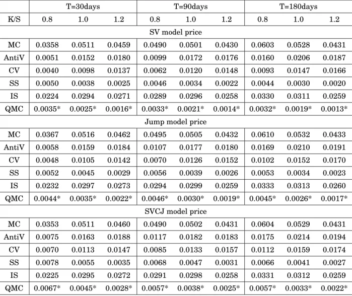
SV model price

MC 0.0358 0.0511 0.0459 0.0490 0.0501 0.0430 0.0603 0.0528 0.0431 AntiV 0.0051 0.0152 0.0180 0.0099 0.0172 0.0176 0.0160 0.0206 0.0187 CV 0.0040 0.0098 0.0137 0.0062 0.0120 0.0148 0.0093 0.0147 0.0166 SS 0.0050 0.0038 0.0025 0.0046 0.0034 0.0022 0.0044 0.0030 0.0020 IS 0.0224 0.0294 0.0271 0.0289 0.0296 0.0258 0.0330 0.0311 0.0259 QMC 0.0035* 0.0025* 0.0016* 0.0033* 0.0021* 0.0014* 0.0032* 0.0019* 0.0013*

Jump model price

SVCJ model price

MC means standard Monte Carlo without variance reduction; * denotes the lowest SE

(57)

500 1000 1500 2000 2500 3000 3500 4000 4500 5000 0 0.5 1 1.5 2 2.5 3 RMSE: SV,K/S=0.8,T=30 Simulation Number RMSE MC AntiV CV SS IS QMC

500 1000 1500 2000 2500 3000 3500 4000 4500 5000 0 0.5 1 1.5 2 2.5 RMSE: SV,K/S=1.0,T=30 Simulation Number RMSE MC AntiV CV SS IS QMC

500 1000 1500 2000 2500 3000 3500 4000 4500 5000 0 0.5 1 1.5 2 2.5 3 3.5 RMSE: SV,K/S=1.2,T=30 Simulation Number RMSE MC AntiV CV SS IS QMC

500 1000 1500 2000 2500 3000 3500 4000 4500 5000 0 0.5 1 1.5 2 2.5 3 3.5 4 RMSE: SV,K/S=0.8,T=90 Simulation Number RMSE MC AntiV CV SS IS QMC

500 1000 1500 2000 2500 3000 3500 4000 4500 5000 0 0.5 1 1.5 2 2.5 3 3.5 4 4.5 RMSE: SV,K/S=1.0,T=90 Simulation Number RMSE MC AntiV CV SS IS QMC

500 1000 1500 2000 2500 3000 3500 4000 4500 5000 0 0.5 1 1.5 2 2.5 3 3.5 RMSE: SV,K/S=1.2,T=90 Simulation Number RMSE MC AntiV CV SS IS QMC

500 1000 1500 2000 2500 3000 3500 4000 4500 5000 0 1 2 3 4 5 6 RMSE: SV,K/S=0.8,T=180 Simulation Number RMSE MC AntiV CV SS IS QMC

500 1000 1500 2000 2500 3000 3500 4000 4500 5000 0 0.5 1 1.5 2 2.5 3 3.5 4 4.5 RMSE: SV,K/S=1.0,T=180 Simulation Number RMSE MC AntiV CV SS IS QMC

500 1000 1500 2000 2500 3000 3500 4000 4500 5000 0 0.5 1 1.5 2 2.5 3 3.5 4 RMSE: SV,K/S=1.2,T=180 Simulation Number RMSE MC AntiV CV SS IS QMC

(58)

500 1000 1500 2000 2500 3000 3500 4000 4500 5000 0 0.1 0.2 0.3 0.4 0.5 0.6 RMSE: Jump,K/S=0.8,T=30 Simulation Number RMSE MC AntiV CV SS IS QMC

(a) Short Term, In-the-money

500 1000 1500 2000 2500 3000 3500 4000 4500 5000 0 0.5 1 1.5 2 2.5 RMSE: Jump,K/S=1.0,T=30 Simulation Number RMSE MC AntiV CV SS IS QMC

(b) Short Term, At-the-money

500 1000 1500 2000 2500 3000 3500 4000 4500 5000 0 0.5 1 1.5 2 2.5 3 3.5 RMSE: Jump,K/S=1.2,T=30 Simulation Number RMSE MC AntiV CV SS IS QMC

(c) Short Term, Out-the-money

500 1000 1500 2000 2500 3000 3500 4000 4500 5000 0 0.2 0.4 0.6 0.8 1 1.2 RMSE: Jump,K/S=0.8,T=90 Simulation Number RMSE MC AntiV CV SS IS QMC

(d) Medium Term, In-the-money

500 1000 1500 2000 2500 3000 3500 4000 4500 5000 0 0.5 1 1.5 2 2.5 3 RMSE: Jump,K/S=1.0,T=90 Simulation Number RMSE MC AntiV CV SS IS QMC

(e) Medium Term, At-the-money

500 1000 1500 2000 2500 3000 3500 4000 4500 5000 0 0.5 1 1.5 2 2.5 3 RMSE: Jump,K/S=1.2,T=90 Simulation Number RMSE MC AntiV CV SS IS QMC

(f) Medium Term, Out-the-money

500 1000 1500 2000 2500 3000 3500 4000 4500 5000 0 0.2 0.4 0.6 0.8 1 1.2 1.4 1.6 1.8 2 RMSE: Jump,K/S=0.8,T=180 Simulation Number RMSE MC AntiV CV SS IS QMC

(g) Long Term, In-the-money

500 1000 1500 2000 2500 3000 3500 4000 4500 5000 0 0.5 1 1.5 2 2.5 3 3.5 4 RMSE: Jump,K/S=1.0,T=180 Simulation Number RMSE MC AntiV CV SS IS QMC

(h) Long Term, At-the-money

500 1000 1500 2000 2500 3000 3500 4000 4500 5000 0 0.5 1 1.5 2 2.5 3 3.5 RMSE: Jump,K/S=1.2,T=180 Simulation Number RMSE MC AntiV CV SS IS QMC

(i) Long Term, Out-the-money

(59)

500 1000 1500 2000 2500 3000 3500 4000 4500 5000 0 0.1 0.2 0.3 0.4 0.5 0.6 0.7 0.8 0.9 1 RMSE: SVCJ,K/S=0.8,T=30 Simulation Number RMSE MC AntiV CV SS IS QMC

500 1000 1500 2000 2500 3000 3500 4000 4500 5000 0 0.5 1 1.5 2 2.5 3 3.5 RMSE: SVCJ,K/S=1.0,T=30 Simulation Number RMSE MC AntiV CV SS IS QMC

500 1000 1500 2000 2500 3000 3500 4000 4500 5000 0 0.5 1 1.5 2 2.5 3 3.5 4 RMSE: SVCJ,K/S=1.2,T=30 Simulation Number RMSE MC AntiV CV SS IS QMC

500 1000 1500 2000 2500 3000 3500 4000 4500 5000 0 0.2 0.4 0.6 0.8 1 1.2 1.4 1.6 1.8 2 RMSE: SVCJ,K/S=0.8,T=90 Simulation Number RMSE MC AntiV CV SS IS QMC

500 1000 1500 2000 2500 3000 3500 4000 4500 5000 0 0.5 1 1.5 2 2.5 3 3.5 RMSE: SVCJ,K/S=0.8,T=180 Simulation Number RMSE MC AntiV CV SS IS QMC

500 1000 1500 2000 2500 3000 3500 4000 4500 5000 0 0.5 1 1.5 2 2.5 3 3.5 4 4.5 RMSE: SVCJ,K/S=1.0,T=180 Simulation Number RMSE MC AntiV CV SS IS QMC

(60)

500 1000 1500 2000 2500 3000 3500 4000 4500 5000 0 0.02 0.04 0.06 0.08 0.1 0.12 SE: SV,K/S=0.8,T=30 Simulation Number RMSE MC AntiV CV SS IS QMC

500 1000 1500 2000 2500 3000 3500 4000 4500 5000 0 0.02 0.04 0.06 0.08 0.1 0.12 0.14 0.16 SE: SV,K/S=1.0,T=30 Simulation Number RMSE MC AntiV CV SS IS QMC

500 1000 1500 2000 2500 3000 3500 4000 4500 5000 0 0.02 0.04 0.06 0.08 0.1 0.12 0.14 SE: SV,K/S=1.2,T=30 Simulation Number RMSE MC AntiV CV SS IS QMC

500 1000 1500 2000 2500 3000 3500 4000 4500 5000 0 0.02 0.04 0.06 0.08 0.1 0.12 0.14 0.16 0.18 0.2 SE: SV,K/S=0.8,T=180 Simulation Number RMSE MC AntiV CV SS IS QMC

(61)

500 1000 1500 2000 2500 3000 3500 4000 4500 5000 0 0.02 0.04 0.06 0.08 0.1 0.12 SE: Jump,K/S=0.8,T=30 Simulation Number RMSE MC AntiV CV SS IS QMC

500 1000 1500 2000 2500 3000 3500 4000 4500 5000 0 0.02 0.04 0.06 0.08 0.1 0.12 0.14 0.16 SE: Jump,K/S=1.0,T=30 Simulation Number RMSE MC AntiV CV SS IS QMC

500 1000 1500 2000 2500 3000 3500 4000 4500 5000 0 0.02 0.04 0.06 0.08 0.1 0.12 0.14 SE: Jump,K/S=1.2,T=30 Simulation Number RMSE MC AntiV CV SS IS QMC

500 1000 1500 2000 2500 3000 3500 4000 4500 5000 0 0.02 0.04 0.06 0.08 0.1 0.12 0.14 0.16 0.18 0.2 SE: Jump,K/S=0.8,T=180 Simulation Number RMSE MC AntiV CV SS IS QMC

(62)

500 1000 1500 2000 2500 3000 3500 4000 4500 5000 0 0.02 0.04 0.06 0.08 0.1 0.12 SE: SVCJ,K/S=0.8,T=30 Simulation Number RMSE MC AntiV CV SS IS QMC

500 1000 1500 2000 2500 3000 3500 4000 4500 5000 0 0.02 0.04 0.06 0.08 0.1 0.12 0.14 0.16 SE: SVCJ,K/S=1.0,T=30 Simulation Number RMSE MC AntiV CV SS IS QMC

500 1000 1500 2000 2500 3000 3500 4000 4500 5000 0 0.05 0.1 0.15 SE: SVCJ,K/S=1.2,T=30 Simulation Number RMSE MC AntiV CV SS IS QMC

500 1000 1500 2000 2500 3000 3500 4000 4500 5000 0 0.02 0.04 0.06 0.08 0.1 0.12 0.14 SE: SVCJ,K/S=1.2,T=90 Simulation Number RMSE MC AntiV CV SS IS QMC

500 1000 1500 2000 2500 3000 3500 4000 4500 5000 0 0.02 0.04 0.06 0.08 0.1 0.12 0.14 0.16 0.18 0.2 SE: SVCJ,K/S=0.8,T=180 Simulation Number RMSE MC AntiV CV SS IS QMC

500 1000 1500 2000 2500 3000 3500 4000 4500 5000 0 0.02 0.04 0.06 0.08 0.1 0.12 0.14 SE: SVCJ,K/S=1.2,T=180 Simulation Number RMSE MC AntiV CV SS IS QMC

(63)

100 200 300 400 500 600 700 0 0.05 0.1 0.15 0.2 0.25

SE by Simulation Number (Optoin:Long Term,Out−the−money)

Simulation Number SE MC AntiV CV SS IS QMC

100 200 300 400 500 600 700 0 0.02 0.04 0.06 0.08 0.1 0.12 0.14 0.16 0.18

100 200 300 400 500 600 700 0 0.002 0.004 0.006 0.008 0.01 0.012 0.014 0.016 0.018 0.02

100 200 300 400 500 600 700 0 0.1 0.2 0.3 0.4 0.5 0.6 0.7

100 200 300 400 500 600 700 0 0.05 0.1 0.15 0.2 0.25 0.3 0.35 0.4 0.45 0.5

100 200 300 400 500 600 700 0 0.02 0.04 0.06 0.08 0.1 0.12 0.14 0.16

100 200 300 400 500 600 700 0 0.1 0.2 0.3 0.4 0.5 0.6 0.7 0.8 0.9 1

100 200 300 400 500 600 700 0 0.1 0.2 0.3 0.4 0.5 0.6 0.7

100 200 300 400 500 600 700 0 0.05 0.1 0.15 0.2 0.25 0.3 0.35