.>;;07= <300=< 47 =30 <85,; .8;87,*
18;6,=487! 1;,2607=,=487 ,7/ 30,=472
;QPF -LSKCOO
, =FCOGO <Q@JGPPCB DLN PFC /CENCC LD 9F/
?P PFC
>KGRCNOGPU LD <P# ,KBNCSO
'%&&
1QII JCP?B?P? DLN PFGO GPCJ GO ?R?GI?@IC GK
;COC?NAF+<P,KBNCSO*1QII=CTP
?P*
FPPM*$$NCOC?NAF"NCMLOGPLNU#OP"?KBNCSO#?A#QH$
9IC?OC QOC PFGO GBCKPGDGCN PL AGPC LN IGKH PL PFGO GPCJ*
FPPM*$$FBI#F?KBIC#KCP$&%%'($'%)&
Current Sheets in the Solar Corona:
Formation, fragmentation and heating
Ruth Bowness
Thesis submitted for the degree of Doctor of Philosophy
of the University of St Andrews
Abstract
In this thesis we investigate current sheets in the solar corona. The well known 1D model for the tearing mode instability is presented, before progressing to 2D where we introduce a non-uniform resistivity. The effect this has on growth rates is investigated and we find that the inclusion of the non-uniform term in
η cause a decrease in the growth rate of the dominant mode. Analytical approximations and numerical simulations are then used to model current sheet formation by considering two distinct experiments. First, a magnetic field is sheared in two directions, perpendicular to each other. A twisted current layer is formed and we find that as we increase grid resolution, the maximum current increases, the width of the current layer decreases and the total current in the layer is approximately constant. This, together with the residual Lorentz force calculated, suggests that a current sheet is trying to form. The current layer then starts to fragment. By considering the parallel electric field and calculating the perpendicular vorticity, we find evi-dence of reconnection. The resulting temperatures easily reach the required coronal values. The second set of simulations carried out model an initially straight magnetic field which is stressed by elliptical boundary motions. A highly twisted current layer is formed and analysis of the energetics, current structures, mag-netic field and the resulting temperatures is carried out. Results are similar in nature to that of the shearing experiment.
Declarations
I, Ruth Bowness, hereby certify that this thesis, which is approximately 45,000 words in length, has been written by me, that it is the record of work carried out by me and that it has not been submitted in any previous application for a higher degree.
I was admitted as a research student in September 2007 and as a candidate for the degree of Doctor of Philosophy in September 2008; the higher study for which this is a record was carried out in the University of St Andrews between 2007 and 2011.
Date: Signature of Candidate: .
I hereby certify that the candidate has fulfilled the conditions of the Resolution and Regulations appro-priate for the degree of Doctor of Philosophy in the University of St Andrews and that the candidate is qualified to submit this thesis in application for that degree.
Date: Signature of Supervisor: .
In submitting this thesis to the University of St Andrews we understand that we are giving permission for it to be made available for use in accordance with the regulations of the University Library for the time being in force, subject to any copyright vested in the work not being affected thereby. We also understand that the title and the abstract will be published, and that a copy of the work may be made and supplied to any bona fide library or research worker, that my thesis will be electronically accessible for personal or research use unless exempt by award of an embargo as requested below, and that the library has the right to migrate my thesis into new electronic forms as required to ensure continued access to the thesis. We have obtained any third-party copyright permissions that may be required in order to allow such access and migration, or have requested the appropriate embargo below.
The following is an agreed request by candidate and supervisor regarding the electronic publication of this thesis:
Access to Printed copy and electronic publication of thesis through the University of St Andrews.
Date: Signature of Candidate: Signature of Supervisor: .
Acknowledgements
Firstly, I would like to thank my supervisor, Alan, for his continued advice and encouragement. My PhD would certainly not have been possible without him. Also thank you to Ineke for inspiring me to come back to St Andrews to do my PhD. Thank you also to Clare for her advice and help with the work in Chapters 4 and 5 and to Andrew for codes to calculate the parallel electric field and Q values.
The simulations presented in the thesis were run on the UK MHD cluster at the University of St. Andrews funded by STFC/SRIF and I would also like to acknowledge PhD funding from STFC.
My friends have been very supportive over the past few years. Faye, thank you for reminding me to ‘just keep swimming’, it has been my mantra. Cicely, Dee, Karen, Lynsey & Solmaz, without our girly nights, circuits sessions, cake eating and eternal joyous dancing I would have found my PhD much harder! Thank you also to my office mates Dee, Lynsey, Alex, Greg & Aimilia for providing useful discussions and sometimes mindless chatter, both were equally important. Also, thanks for looking the other way when I started to talk to myself. To all of my other friends, thank you for allowing me to constantly bore you with details of my thesis.
My Mum and Dad have been a constant form of support throughout my life, always encouraging me to do my best. An ‘A’ for effort is all they ever wanted from me, which I hope I’ve been able to give. Thank you for inspiring me to work hard and for your endless faith in me. James, my husband, has been with me through every step of my degree and my PhD and has shared my stress along the way. I truly couldn’t have done it without you.
I would like to dedicate my thesis to my sister, Kathryn. I made a promise to her that I would complete my PhD and I know that she would be very proud of me now.
Contents
Contents iv
List of Figures vii
1 Introduction 1
1.1 The Solar Corona . . . 1
1.1.1 Coronal Heating . . . 2
1.2 MHD Equations . . . 3
1.2.1 Electromagnetic Equations . . . 3
1.2.2 Summary of the MHD Equations . . . 6
1.2.3 The Induction Equation . . . 6
1.3 Sequences of MHD Equilibria . . . 8
1.4 Current Sheets . . . 9
1.4.1 Current Sheet Formation . . . 9
1.4.2 Current Sheet Properties . . . 10
1.5 Resistive Instabilities . . . 11
1.6 Magnetic Reconnection . . . 13
1.6.1 2D Reconnection . . . 13
1.6.2 3D Reconnection . . . 16
1.7 Outline of Thesis . . . 17
2 Numerical Codes 18 2.1 Introduction . . . 18
2.2 Numerical Techniques . . . 18
2.2.1 Finite Difference Formulae . . . 18
2.2.2 Predictor-Corrector Methods . . . 20
2.3 The LareXd Code . . . 21
2.3.1 The Grid . . . 22
2.3.2 Lagrangian Step . . . 24
2.3.3 The Remap Step . . . 27
2.3.4 Using the Code . . . 28
2.4 Summary . . . 28
3 Modelling the Tearing Mode Instability 29 3.1 Introduction . . . 29
3.1.1 Outline of this Chapter . . . 30
3.2 Tearing Mode Instability in 1D with Uniform Resistivity . . . 31
3.2.1 Simple Order of Magnitude Solution . . . 33
3.2.2 Boundary Layer Analysis . . . 36
3.2.3 Numerical Estimate . . . 42
3.3 Tearing Mode Instability in 2D with a Non-Uniform Resistivity . . . 48
3.3.1 Simple Order of Magnitude Solution . . . 50
3.3.2 Boundary Layer Analysis . . . 53
3.3.3 Numerical Estimate . . . 58
3.4 Using Lare2d to Model the Non-Linear Tearing Mode Instability . . . 61
3.5 Conclusions . . . 66
4 Current Sheet Formation: Boundary Shearing a Magnetic Field 67 4.1 Introduction . . . 67
4.1.1 Outline of this Chapter . . . 68
4.2 Analytical Model . . . 69
4.2.1 First Shear . . . 69
4.2.2 Second Shear . . . 69
4.3 Numerical Simulation . . . 76
4.3.1 Numerical Model . . . 76
4.3.2 Initial Magnetic Field: First shear . . . 77
4.3.3 Drivers: Second shear . . . 78
4.3.4 Evolution of Magnetic Field . . . 80
4.3.5 Energy: Total Energy and Poynting Flux . . . 84
4.3.6 Current Layer Structure . . . 90
4.4 Conclusions . . . 99
5 Analysis of the Temperatures, Current Sheet Fragmentation and Reconnection 101 5.1 Introduction . . . 101
5.1.1 Outline of this Chapter . . . 102
5.2 Plasma Beta . . . 103
5.3 Temperature Response of the Plasma . . . 103
5.4 Current Fragmentation . . . 108
5.5 E Parallel . . . 110
5.6 Flows . . . 114
5.6.1 Vorticity . . . 115
5.7 Q Values . . . 118
5.8 Relaxation . . . 121
5.8.1 Helicity . . . 123
5.9 Conclusions . . . 126
6 Current Sheet Formation: Elliptical Boundary Motions applied to a Magnetic Field 128 6.1 Introduction . . . 128
6.1.1 Outline of this Chapter . . . 128
6.2 Numerical Model . . . 128
6.2.1 Equations . . . 128
6.2.2 Boundary Conditions . . . 129
6.3 Boundary Motions . . . 129
6.3.1 Driver . . . 131
6.3.2 Movement of the Fluid Elements . . . 132
6.4 Evolution of the Magnetic Field . . . 133
6.5 Energetics . . . 134
6.6 Current Layer Structure . . . 136
6.7 Magnetic Structure . . . 138
6.8 Temperatures . . . 140
6.9 Conclusions . . . 141
7 Conclusions and Future Work 142 7.1 Overview of Thesis . . . 142
7.2 Summary of Results . . . 142
7.3 Future Work . . . 145
A Solution to Eq. (3.19) 146
Bibliography 150
List of Figures
1.1 Left: The solar corona viewed from the top of Mauna Kea, Hawaii during a total solar eclipse in 1991. (NASA Astronomy Picture of the Day). Right: Corona viewed with
LASCO C2 coronagraph in 1997. (NASA Best of SOHO gallery). . . 1
1.2 The changing temperature from the solar surface out into the corona. A minimum of about 4300K is reached in the photosphere. The temperature then rises to about 20,000K at the top of the chromosphere, before surging to over106K in the corona. . . . 2
1.3 The collapse of an X-point to form a current sheet. . . 9
1.4 How the tearing mode instability forms. . . 11
1.5 The tearing mode instability. Magnetic X-points and O-points are formed at the boundary between regions of oppositely directed field, with plasma flow in the directions indicated by the bold arrows. . . 12
1.6 Sweet-Parker reconnection. The diffusion region is shaded. The plasma velocity is indi-cated by bold arrows and the magnetic field lines by light arrows. . . 13
1.7 Petschek’s model. The central shaded region is the diffusion region and the slow mode shocks are highlighted by the dashed lines. The plasma velocity is indicated by bold arrows and the magnetic field lines by light arrows. . . 15
2.1 Position of variables defined on a 1D grid. . . 23
2.2 Position of variables defined on a 2D grid. . . 23
2.3 Position of variables defined on a 3D grid. . . 23
3.1 Growth Rate forBy = tanh(x)for0< k <1, whereη = 0.01is shown by the solid line, η= 0.001by the dotted line andη= 0.0001by the dashed line. . . 41
3.2 Growth rate plotted for0< k <1with (a)η = 0.01, (b)η = 0.001and (c)η = 0.0001. The dashed line shows the corresponding analytical growth rate calculated by Eq. (3.21) and the dotted line indicateskmfor each case. (d) shows a log-log plot of the numerical growth rate with fixedk= 0.5against various values ofη. . . 44
3.3 Growth rate plotted for0 < k <1with (a)η = 0.001and (b)η = 0.0001, now with the extra solution added in. The dashed line shows the corresponding analytical growth rate calculated by Eq. (3.21) and the dotted line indicates the previous analytic solution (see Fig. 3.2(b),(c)). . . 46
3.4 (a) The Eigenvalues of the matrixM, (b) the growth rates, σand (c) the boundary layer thickness,#are plotted as functions ofη1. Mode 1 is shown by the solid line, mode 2 by the dotted line and mode 3 by the dashed line. . . 52
3.5 Growth Rate as a function ofη1fork= 0.1. Mode 1 is shown by the solid line, Mode 2 by
the dotted line and Mode 3 by the dashed line. . . 57
3.6 (a) Growth Rates as functions ofη1fork= 0.1. (b) Growth Rates as functions ofη1, where
an arbitrary constant is added to the analytical growth rate to compare the gradient of the two estimates. The solid line shows the numerical estimate for the growth rates and the dotted line shows the boundary layer approach results. . . 58
3.7 Growth Rate as a function ofη1fork = 0.1. Solid line shows the coupling effects asη1
increases. The dashed line shows the numerical result of the growth rate with the uniform resistivity,η=η0+η1. . . 59
3.8 Contour plots of the magnetic field, with 8 levels between 0and0.08, whenη0 = 0.001
with (a)η1= 0, (b)η1= 0.00001, (c)η1= 0.00005and (d)η1= 0.0001. . . 60
3.9 Initial profile ofbx(a) aty= 0as a function ofxand (b) atx= 0as a function ofy. . . . 62
3.10 Initial profile ofby(a) aty= 0as a function ofxand (b) atx= 0as a function ofy. . . . 62
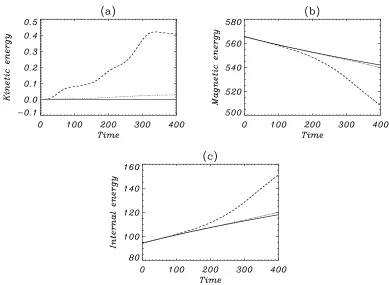
3.11 The volume integrated energies (a) kinetic, (b) magnetic and (c) internal as functions of time. The solid line denotesη1= 0, the dottedη1= 0.001and the dashedη1= 0.0005. . . 63
3.12 Contour plots of the magnetic field at time t = 400, with100 levels between0 and20, when (a)η1= 0, (b)η1= 0.0001and (c)η1= 0.0005. . . 64
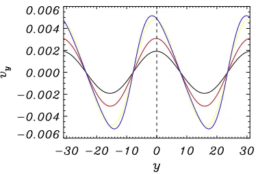
3.13 vyas a function ofyat timest= 100(black),t= 200(red),t= 300(yellow) andt= 400
(blue). The dashed line indicatesy= 0. . . 65
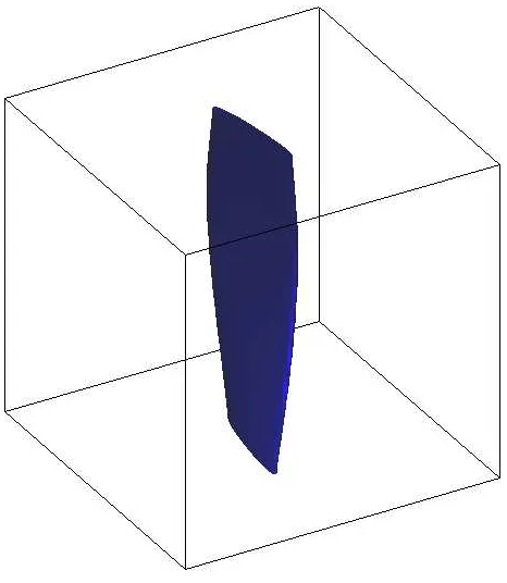
4.1 Isosurface of the current calculated analytically. . . 75
4.2 (a) Plot of the temporal part ofvx,f(t), as a function of time. (b) Temporal displacement,
D(t), achieved with the second shear. The solid line indicates driver 1 and the dashed line indicates driver 2. . . 80
4.3 Contour plots of the current magnitude in the mid-plane, z = 0for, times 0, 5, 7 and 10 ((a)-(d), respectively) are shown for driver 1 andη= 0with a grid resolution of5123. Red corresponds to a maximum of 400 while blue corresponds to a minimum value of1. . . . 81
4.4 Maximum current in the domain as a function of time for both drivers withη = 0and a grid resolution of 5123. Driver 1 is shown by the solid line and the diamonds mark each
time the current was calculated. Driver 2 is shown by the dashed line and the squares show each time the current was calculated. . . 82
4.5 As for Fig. 4.3 att= 7(a) andt= 10(b), but with driver 2,η= 0and a grid resolution of
5123. Red corresponds to a maximum of 400 while blue corresponds to a minimum value
of1. . . 82
4.6 As for Fig. 4.3 att= 10andη= 0, but with driver 1 (a) and driver 2 (b). Arrows show the horizontal velocity with the length of the arrows related to the magnitude of the velocity. . 83
4.7 The volume integrated energies (a) kinetic, (b) internal, (c) magnetic and (d) total energy as functions of time forη = 0and driver 1 (solid) and driver 2 (dashed). For the driver 2 run, the start (asterisk) of the ramp down and end (triangle) of the ramp down of driver 2 are indicated. This experiment was carried out with a grid resolution5123. . . . 85
4.8 The instantaneous negative Poynting flux (driver 1 - plus signs and driver 2 - asterisks) and the rate of change in the total energy,detot/dt, (driver 1 - solid and driver 2 - dotted line)
versus time. This experiment was carried out with a grid resolution of5123. . . 86
4.9 The volume integrated (a) kinetic, (b) internal, (c) magnetic and (d) total energies versus time for experiments with driver 1 and resistivities ofη= 0(solid),η= 10−5(dotted) and
η= 10−4(dashed). This experiment was carried out with a grid resolution of5123. . . . . 88
4.10 Maximum current magnitude is shown as a function of time for the driver 1 experiments with a5123grid forη= 0(black, triangles),η = 10−5(red, squares) andη= 10−4(blue, crosses). The symbols correspond to the times at which the current is actually calculated in each experiment. . . 89
4.11 The negative Poynting flux and the rate of change in the total energy (detot/dt) are shown as
functions of time with a5123grid forη= 0(black, plus signs),η= 10−5(red, diamonds)
andη= 10−4(blue, asterisks). . . . 90
4.12 Isosurface of current at13%of the maximum current magnitude at time (a)t= 7and (b)
t= 8for the driver 1 experiment withη= 0and a grid resolution of5123. . . . 91
4.13 Plots of current for the driver 1 experiment withη = 0and a grid resolution of5123taken
at timet = 7. jz at the mid-plane (a) across the layer (y = 0) and (b) along the layer
(x= 0). (c)jzthrough the centre of the layer, along its height (x=y= 0). . . 92
4.14 Maximum of the current in the domain over the whole simulation versus grid resolution for the driver 1 experiment withη= 0. . . 93 4.15 [j×B]xacross the layer (y= 0) at the mid-plane at t=7. Notice that here−0.02< x <0.02
to highlight the nonzero behaviour. The experiment is the driver 1,η = 0case with5123
grid resolution. . . 94
4.16 j/j!as a function of time, in the range5.5< t <7.0. The experiment is the driver 1,η= 0
case with5123grid resolution. . . . 94
4.17 Slices of the current magnitude in horizontal planes (a)z= 0, (b)z= 0.2and (c)z= 0.4. The arrows denote the vector[Bx, By,0]. The experiment is the driver 1,η= 0case with a
grid resolution of5123. Red corresponds to a maximum of 100 while blue corresponds to
a minimum value of 0. . . 96
4.18 Magnetic fieldlines drawn from starting points along the line−0.2 < y < 0.2atz = 0,
x= 0.01(red lines) andx=−0.01(green lines) att= 7taken from the experiment using driver 1,η= 0and5123resolution. . . . 97
4.19 Current layer angle as a function of z usingy = 0.05. This is taken att = 7with the experiment using driver 1,η= 0and5123resolution. . . 97 4.20 The magnetic field components are plotted att= 7across the layer (y=0) at the mid-plane.
BxandBy are shown in (a), where the solid line corresponds toBy and the dashed line
denotesBx.Bzis shown in (b) and (c) shows the total pressure. These are taken att= 7
with the experiment using driver 1,η= 0and5123resolution. . . . 98
4.21 A perpendicular cut across the layer atz = 0.2of the normal and tangential components of Bare plotted in (a). The solid lines correspond toBy andBx while the dashed lines
denoteB||andB⊥. The total pressure is also plotted perpendicular to the current layer in (b), this is shown by the dashed line, the solid line represents the total pressure taken at the mid plane. Note that these plots are over a range −0.1 < x < 0.1as only a cut of this length was calculated. These are taken att= 7with the experiment using driver 1,η = 0
and5123resolution. . . . 99
5.1 Evolution of the maximum value ofβover time. The black line corresponds toη= 0, the red toη= 10−5and the blue toη= 10−4. The symbols represent each time the plasmaβ
was calculated. Driver 1 and a grid resolution of5123was used. . . 103
5.2 The temperature atx =y =z = 0as a function of time. The black line corresponds to
η= 0, the red toη= 10−5and the blue toη= 10−4. The symbols represent each time the
temperature was calculated. Driver 1 and a grid resolution of5123was used. . . 104
5.3 The temperature at x = y = z = 0 as a function of time withη = 10−4 and a grid
resolution of5123. The symbols denote each time the temperature was calculated. . . 104
5.4 Temperature at x=y = 0as a function of height,zat timest = 7(solid line),t = 7.5
(dotted line),t = 8(dashed line) andt = 8.5(dot-dashed line) forη = 10−4 and a grid
resolution of5123. . . 105
5.5 Isosurfaces of temperature at value=0.3 for η = 10−4at times t = 7,7.5,8,8.5, (a)-(d)
respectively. A grid resolution of5123was used. . . 106
5.6 Slices of temperature atz= 0forη= 10−4at timest= 7,7.5,8,8.5, (a)-(d) respectively.
Blue corresponds to 0 and red to 0.3. A grid resolution of5123was used. . . 107
5.7 Maximum current in the domain as a function of time, forη= 10−4and a grid resolution
of5123. The symbols denote each time the current was calculated. . . 108
5.8 Slices of current magnitude atz = 0for timest = 7,7.5,8,8.5, (a)-(d) respectively. η = 10−4and a grid resolution of5123was used. Blue corresponds to a minimum of 0 and red
to 200. The arrows denote the vector[vx, vy,0]. . . 109
5.9 Absolute value of the parallel electric field integrated along a field line atx=y = 0as a function of time withη= 10−4and a grid resolution of5123. . . 110
5.10 Absolute value of the parallel electric field at x = y = 0 as a function of z at times
t= 7,7.5,8,8.5, (a)-(d) respectively, withη= 10−4and a grid resolution of5123. . . 111
5.11 Absolute value of the parallel electric field at x = z = 0 as a function ofy at times
t= 7,7.5,8,8.5, (a)-(d) respectively, withη= 10−4and a grid resolution of5123. . . 112
5.12 Absolute value of the parallel electric field at y = z = 0 as a function of xat times
t= 7,7.5,8,8.5, (a)-(d) respectively, withη= 10−4and a grid resolution of5123. . . 112
5.13 Magnetic field lines drawn from starting points along a line−0.2< y <0.2atx=z= 0, coloured by|E|||at timest= 7,7.5,8,8.5, (a)-(d) respectively. The blue corresponds to a
value of0and the red to0.02. . . 113
5.14 Velocity components, (a)vxas a function ofx, (b)vy as a function ofy and (c)vz as a
function of zat timest = 7(solid line),t = 7.5(dotted line), t = 8(dashed line) and
t= 8.5(dot-dashed line). η= 10−4and a grid resolution of5123was used. . . 114 5.15 [ω⊥]zatx=y = 0as a function ofzatt= 7,7.5,8,8.5, (a)-(d) respectively. η= 10−4
and a grid resolution of5123was used. The star symbol indicates locations where there is
a change of sign inω⊥. . . 115 5.16 [ω⊥]zatx=z = 0as a function ofyatt= 7,7.5,8,8.5, (a)-(d) respectively. η= 10−4
and a grid resolution of5123was used. The star symbol denotes locations where there is a
change of sign inω⊥. . . 116 5.17 [ω⊥]zaty =z = 0as a function ofxatt= 7,7.5,8,8.5, (a)-(d) respectively. η= 10−4
and a grid resolution of5123was used. The star symbol denotes locations where there is a
change of sign inω⊥. . . 117 5.18 [ω⊥]zatz = 0,0.067,0.157,0.229(locations of highest absolute parallel electric field) at
timest = 7,7.5,8,8.5, (a)-(d) respectively. η = 10−4and a grid resolution of5123was
used. Red corresponds to a maximum of 75 and blue to a minimum of -75. . . 117
5.19 Plots of Q for z=0.0,0.2,0.4 (top to bottom). . . 120
5.20 Magnetic fieldlines drawn from starting points along a line−0.2 < y < 0.2 atx = 0,
z = 0at a time t=25.0. Driver 1 is shown in (a) and driver 2 in (b), both experiments are withη= 0and grid resolution5123. . . 121
5.21 Magnetic field components at the mid-plane shown across the layer at timet= 25(a)Bx,
(b)By and (c)Bz. The dotted line shows the field components when driver 1 is used, the
dashed line shows driver 2. The solid line denotes the initial magnetic field after the first shear, i.e. B =!0,λsin"πx
w
#
,$"
1 +λ2cos2"πx w
##%
. Experiments are withη = 0and grid resolution5123. . . 122
5.22 The relative helicity in the system when driver 1 is used (left) and driver 2 is used (left). . . 125
6.1 Elliptical motions imposed on the top (left) and the base (right) of the numerical box. . . . 131
6.2 Slices of the current magnitude atz = 0at times (a)t= 0, (b)t= 15, (c)t = 40and (d)
t= 65forη = 0. Blue corresponds to a minimum value of 0 and red to a maximum value 40. A grid resolution of3523was used. . . 133
6.3 Maximum current in the domain as a function of time withη = 0(black),η = 10−4(red)
andη= 5×10⁻⁴(blue). A grid resolution of3523was used. The symbols mark each time
the current was calculated. . . 134
6.4 Volume integrated energies (a) kinetic, (b) internal, (c) magnetic and (d) total energy as functions of time forη= 0(solid),η = 10−4(dotted) andη= 5×10⁻⁴(dashed). A grid
resolution of3523was used. . . 135
6.5 The instantaneous negative Poynting flux and the rate of change in the total energy,detot/dt,
versus time with a3523grid forη= 0(black, plus signs),η = 10−4(red, diamonds) and
η= 5×10⁻⁴(blue, asterisks). . . 135
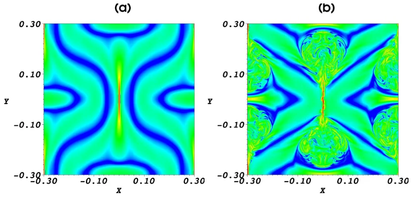
6.6 Isosurface at20%of the maximum current magnitude att= 40forη= 0. A grid resolution of3523was used. . . 136
6.7 Slice of the current magnitude atz =−1with the arrows denoting the vector[Bx, By,0]
taken at timet = 40forη = 0. Blue corresponds to a minimum value of 0 and red to a maximum of 40. A grid resolution of3523was used. . . 137 6.8 Plots of current withη= 0and a grid resolution of3523taken at timet= 40.j
zatz=−1
(a) across the layer (y = 0) and (b) along the layer (x= 0). Notice here that we focus on the central area of the box,−0.4< x, y <0.4. . . 137
6.9 [j×B]xacross the layer (y = 0) atz =−1att= 40. Notice here that we focus on the
central area of the box, −0.4 < x < 0.4. The experiment is with η = 0and3523 grid
resolution. . . 138
6.10 The magnetic field components att= 40are shown across the layer aty = 0,z =−1in (a)Bx, (b)By, (c)Bzand (d) Total pressure forη= 0. A grid resolution of3523was used.
Notice here that we focus on the central area of the box,−0.4< x <0.4. . . 139
6.11 Magnetic fieldlines drawn from starting points along the line−0.2< y <0.2atz =−1,
x= 0.02(red lines) andx=−0.02(green lines) att= 40taken from the experiment with
η= 0and3523resolution. . . 140
6.12 The temperature atx =y = z = 0as a function of time withη = 0(black),η = 10−4
(red) andη = 5×10⁻⁴(blue). A grid resolution of3523was used. The symbols denote
each time the temperature was calculated. . . 140
Chapter 1
Introduction
1.1
The Solar Corona
This thesis aims to investigate current sheets in the solar corona. Analytical approximations and numerical simulations will be used to discuss how they form, how they can become unstable and fragment and how this process can cause magnetic reconnection and heating.
There are three distinct regions in the atmosphere of the Sun. The lowest level is the visible surface of the Sun, the photosphere. This layer is very thin, with a thickness of about 500 km. The temperature in the photosphere falls to a minimum of 4300 K where it unexpectedly begins to rise again, marking the boundary between the photosphere and the chromosphere. The temperature rises slowly through the chromosphere until there is a rapid rise to the corona, where the temperature is much hotter at over a million K. This thin region of temperature increase from the chromosphere to the corona is known as the transition region and can range from tens to hundreds of kilometres thick.
The corona can only be seen when the disk of the Sun is blocked off in a total solar eclipse, or by using a special instrument called a coronagraph that artificially blocks the disk of the Sun so that it can image the surrounding regions. Fig. 1.1(left) shows the corona, appearing as a halo around the main body of the Sun, during a total solar eclipse and Fig. 1.1(right) shows the corona using a the Large Angle and Spectrometric Coronagraph (LASCO) onboard the Solar and Heliospheric Observatory (SoHO) spacecraft.
Fig. 1.1: Left: The solar corona viewed from the top of Mauna Kea, Hawaii during a total solar eclipse in 1991. (NASA Astronomy Picture of the Day). Right: Corona viewed with LASCO C2 coronagraph in 1997. (NASA Best of SOHO gallery).
1.1 The Solar Corona 2
[image:16.612.218.430.127.338.2]1.1.1 Coronal Heating
Fig. 1.2 illustrates the temperature change from the photosphere out to the corona.
Fig. 1.2: The changing temperature from the solar surface out into the corona. A minimum of about 4300K is reached in the photosphere. The temperature then rises to about 20,000K at the top of the chromosphere, before surging to over106K in the corona.
Physical intuition tells us that as we move away from the heat source at the centre of the Sun, tempera-tures should decrease. This is not the case, the corona is incredibly hot at a temperature above one million degrees Kelvin. The main cooling mechanisms at this temperature and low density are optically thin radia-tion and thermal conducradia-tion parallel to the magnetic field. The timescale for radiative cooling is the order of3,000s and the conduction timescale is of the order of500s. Hence, heat must be fed into the corona on at least this timescale and there must be a continual input of heat or the plasma would cool down in about an hour. Withbroe and Noyes (1977) estimated that300Wm−2is required to heat the quiet Sun and
5,000Wm−2to heat active regions. The permanent energy source must lie in the solar interior. By means
of a Poynting flux calculation, the flow of magnetic energy from the interior to the corona was calculated in Hood (2010) to be≈104Wm−2, hence the energy is sufficient for heating.
There must also be a mechanism to convert the stored magnetic energy into heat. MHD waves and magnetic reconnection are two possible ways in which the energy is dissipated. Which mechanism plays a role is dependent on the time scale of the photospheric motions (τ). Let the length of a typical coronal loop beLand the Alfv´en velocity bevA. Then ifτis less thanL/vA, the motions are considered rapid and
MHD waves propagate upwards, whereas slow motions (τ > L/vA) result in the storage of energy in the
1.2 MHD Equations 3
1.2
MHD Equations
1.2.1
Electromagnetic Equations
1.2.1.1 Maxwell’s Equations
Maxwell’s Equations are as follows:
Amp`ere’s Law:
∇×B=µj+ 1
c2
∂E
∂t, (1.1)
where the last term on the right hand side is the displacement current. Amp`ere’s Law tells us that gradients in the magnetic field create electric currents.
Solenoidal constraint:
∇·B= 0, (1.2)
which implies there are no magnetic monopoles, i.e., no sources or sinks of magnetic field. Faraday’s Law:
∇×E=−∂B
∂t, (1.3)
which indicates that spatially varying electric field can induce a magnetic field. Gauss’ Law:
∇·E=1
#ρ
∗, (1.4)
implying charge conservation.
For these equations we useB, magnetic induction, but it is usually referred to as magnetic field;j, the current density;E, the electric field;ρ∗=e(n+−n−), the charge density (wheren+is the number of ions
andn− is the number of electrons per unit volume in a fully ionised hydrogen plasma);#, permittivity of
free space;µ, magnetic permeability in a vacuum (4π×10−7Hm−1) andc= (µ#)−1/2≈3×108ms−1,
the speed of light in a vacuum.
1.2.1.2 Assumptions of MHD
• The theory is macroscopic: the typical length scale,l0, of the spatial variations and time scale,τ, of
1.2 MHD Equations 4
collision dominated.
• The displacement current in Amp`ere’s law may be neglected if the typical plasma velocities are much less than the speed of light,c. This can be demonstrated as follows, assume a typical length scalel0,
timescalet0and plasma velocityv0=l0/t0. Then, Eq. (1.3) implies
|∇ ×E|≈ E
l0
and∂B
∂t ≈ B t0
.
So we have
E = l0
t0
B=v0B.
Eq. (1.1) also implies
∇ ×B≈B l0 and
1 c2 ∂E ∂t ≈ 1 c2 E t0 =
v0
c2
B t0 =
v0
c2
l0
t0
B l0 =
v20
c2
B l0.
Hence ifv2
0%c2then
[∇ ×B|& 1 c2
∂E ∂t.
The theory is hence non-relativistic and this is known as the MHD approximation. Amp`ere’s law then becomes
∇ ×B=µj.
• The plasma obeys charge neutrality,n+−n− % n, wherenis the total number density. We can
neglect the charge density in Eq. (1.4) provided
n&#Bv0
el0
.
eis the charge on an electron.
1.2.1.3 Ohm’s Law
The final electromagnetic equation is Ohm’s law,
j=σ(E+v×B), (1.5)
1.2 MHD Equations 5
1.2.1.4 Fluid Equations
Mass continuity:
∂ρ
∂t +∇·(ρv) = 0, (1.6)
whereρis the mass density. It states that matter is neither created nor destroyed. If plasma is incompress-ible,Dρ/Dt= 0, then Eq. (1.6) reduces to∇·v = 0, i.e. there are no sources or sinks inv. Note that
D/Dtis the convective time derivative
D Dt =
∂
∂t +v·∇,
that describes the time derivative of a quantity as it moves with the plasma. Equation of motion:
ρDv
Dt =−∇p+j×B+ρg, (1.7)
wherepis the pressure,j×Bis the the Lorentz force and ρgis the gravitational force. A viscous force could also be added (although we ignore viscous forces in this thesis, except in artificial shock viscosities). Energy equation:
ργ γ−1
D Dt
&
p ργ
'
=−L. (1.8)
HereLis the total energy loss function,γis the ratio of specific heats,cp/cvand is normally taken as 5/3.
Noting thatcpis the specific heat at constant pressure andcvis the specific heat at constant volume.
The energy equation can be written in many different forms. In the coronaL, the energy loss function, consists of three terms; energy loss/gain from thermal conduction, energy loss from optically thin radiation and energy gain from heating. Hence
L=−∇·(κ∇T) +ρ2Q(T)−H,
whereκis the anisotropic thermal conductivity tensor,Q(T)is the optically thin radiative loss function and
His the coronal heating term.
In many solar situations, for ideal cases, we may neglect these terms, setL = 0 and consider the evolution to be adiabatic. In that case, Eq. (1.8) becomes
D Dt
& p
ργ
' = 0.
Using Eq. (1.6), we can write this as
∂p
∂t +v·∇p= γp
ρ
&
∂ρ
∂t + (v·∇)ρ
'
1.2 MHD Equations 6
The last fluid equation is an equation of state that is used to close the system of equations. Ideal Gas Law:
p=ρRT ˜
µ , (1.9)
whereT is the plasma temperature, R = 8.3×10³J K−1kg−1is the gas constant,µ˜is the mean atomic
weight which is usually taken to be0.6in the solar corona. (µ˜= 0.5for a fully ionised hydrogen plasma).
Eq. (1.9) can be written in terms of the number density sinceρ=nmpand so
p=nkBT ˜
µ , (1.10)
wherempis the mass of a proton andkBis Boltzmann’s constant.
1.2.2
Summary of the MHD Equations
The following are the inviscid, adiabatic form of the MHD equations:
∂ρ
∂t +∇·(ρv) = 0, (1.11)
ρ∂v
∂t +ρ(v·∇)v=−∇p+j×B+ρg, (1.12)
∂p
∂t +v·∇p=−γp∇·v+ j2
σ, (1.13)
p=ρRT ˜
µ , (1.14)
j=∇×B/µ, (1.15)
∇·B= 0, (1.16)
∂B
∂t =−∇×E, (1.17)
1
σj=E+v×B. (1.18)
1.2.3
The Induction Equation
In solar MHD, we can eliminate the electric field,E, and the electric current density,jand work with the primary variable,B. To eliminateE, we use Ohm’s law, Eq. (1.18), and Amp`ere’s Law, Eq. (1.15) to get
E=−v×B+ 1
1.2 MHD Equations 7
and so Faraday’s Law, Eq. (1.17), becomes
∂B
∂t =∇×(v×B)−∇×(η∇×B), (1.19)
where
η= 1
µσ,
is the magnetic diffusivity. Whenηis constant, Eq. (1.19) becomes
∂B
∂t = ∇×(v×B)−η∇×(∇×B),
= ∇×(v×B) +η(
∇2B−∇(∇.B))
.
Using the solenoidal constraint, Eq. (1.16), we get the induction equation,
∂B
∂t =∇×(v×B) +η∇
2B, (1.20)
where the term∇×(v×B)is known as the advection term andη∇2Bis known as the diffusion term.
1.2.3.1 Magnetic Reynolds Number
The magnetic Reynolds number, Rm, is the ratio of the advection and diffusion terms in the induction
equation.
Rm =
∇×(v×B)
η∇2B ,
= v0B/l0
ηB/l2 0
,
= l0v0
η = l2
0
ηt0
. (1.21)
Rmis a dimensionless quantity and on the Sun is normally very large (asl0andv0are typically very
large). So in general solar situations,Rm&1, the diffusion term is negligible and so the induction equation
is approximated by
∂B
∂t =∇×(v×B).
However when length scales become small and we haveRm%1, the induction equation reduces to
∂B ∂t =η∇
1.3 Sequences of MHD Equilibria 8
1.3
Sequences of MHD Equilibria
Many physical processes studied in solar physics occur slowly, i.e. on timescales much longer than the typical timescale of the system, so the evolution of these systems can be modelled with a sequence of static equilibria. The theory of static solutions of the MHD equations is called magnetohydrostatics.
Consider the equation of motion, Eq. (1.12),
ρ∂v
∂t +ρ(v·∇)v=−∇p+j×B+ρg.
To derive the magnetohydrostatic equations we neglect flows and assume there is no time variation, so
v= 0and∂/∂t= 0. The result is the magnetohydrostatic balance
0=−∇p+j×B+ρg, (1.22)
between the pressure gradient, the Lorentz force and the gravitational force.
This is coupled with
∇·B= 0, µj=∇×B, p=ρRT ˜
µ ,
whereTsatisfies an energy equation. For simplicity we assume that the temperature is known.
In many applications not all the terms in Eq. (1.22) are equally important. The force of gravity may be neglected by comparison with the pressure gradient when the height of a structure is much less than the scale-height. For example, the large scale-height in the solar corona means that gravity can be neglected. In addition, when the ratio
β =2µp0
B2 0
of plasma to magnetic pressure is much smaller than unity, any pressure gradient is dominated by the Lorentz force.
Eq. (1.22) then reduces to
j×B=0.
Magnetic fields satisfying this condition are called force-free.
1.4 Current Sheets 9
1.4
Current Sheets
As stated above, in the solar atmosphere, the length-scale (l0) over which the magnetic field varies is rather
large, typically 1000−10,000 km (Priest, 1982), and the corresponding current density is very small. However, current sheets are structures with thickness much smaller thanl0and the corresponding current
density is much larger. A current sheet may be defined as a boundary between two plasmas, where the magnetic field on either side is tangential to the boundary and involves a change of direction of the magnetic field. Another condition is that across the sheet, the total pressure (gas plus magnetic) must be continuous. From Amp`ere’s Law, Eq. (1.15), the gradients in magnetic field create a accumulation of electric current which is confined to the infinitesimally thin current sheet.
1.4.1 Current Sheet Formation
The ways in which current sheets form is discussed at length in Priest and Forbes (2000). Here we out-line some 2D analytical models that were developed between 1965-1995. More recently, there have been many more analytical and numerical studies which investigate current sheet formation in two and three dimensions.
y
x
L
−L
−L L
(c) (b)
(a)
Fig. 1.3: The collapse of an X-point to form a current sheet.
The analytical 2D model of current sheets formed by the collapse of an X-point (a type of null or neutral point where the magnetic field vanishes) involves complex-variable theory. For example, consider a potential field X-point (Fig. 1.3(a)) having a fieldBy+iBx=z. If the footpoints of a finite region are
moved or, if a finite energy is added to this minimum-energy configuration and the topology of the field is preserved, the field will evolve to a new configuration. Green (1965) suggested an evolution to a field of the form (Fig.1.3(b)),By+iBx ="z2+L2#
1/2
, having a current sheet stretching fromz =−iLto
z=iL. Somov and Syrovatskii (1976) described the collapse of a two-dimensional X-point with a more general solution
By+iBx=
z2+a2
(z2+L2)1/2,
1.4 Current Sheets 10
to Green’s solution whena2=L2.
This basic theory has been extended in many ways. First of all, the form ofBy+iBx=f(z)has been
written down for other configurations and Titov (1992) proposed a general method for findingf(z)when the topology is preserved. Bungey and Priest (1995) also extended the solution of Somov and Syrovatskii (1976), providing an analytical description for potential and force-free configurations,
By+iBx=−B0
bd2+ 2dcz−z2+1
2d
2
(z2+a2)1/2
,
whereb,c,dandB0are all constants.
The above theory has been applied to more general planar current sheets in the potential and force-free solar corona, involving the magnetic field associated with two bipolar regions, by Priest and Raadu (1975) and Tur and Priest (1976). In these models, a curved current sheet replaces the linear current sheet found in previous studies.
A discussion of more recent literature can be found in chapter 4.
1.4.2 Current Sheet Properties
Priest (1982) describes the main properties of current sheets:
• In the absence of flow, a current sheet diffuses away at a speedη/l. The magnetic field is annihilated (oppositely directed field lines cancel with each other) and magnetic energy converted into heat by ohmic dissipation.
• The region outside a current sheet is effectively frozen to the plasma. Plasma and magnetic flux may be brought towards the sheet from the sides at speedvi. Ifvi <η/lthe sheet expands, whereas if
vi>η/lthe sheet will become thinner. Whenvi=η/la steady state is maintained.
• The enhanced plasma pressure in the centre of the sheet expels material from the ends of the sheet at the Alfv´en speed
&
vA=
B
õ
0ρ
'
based on the reconnecting component of the external magnetic
field and internal density. Magnetic flux is ejected with the material, and so one effect of the sheet is to reconnect the field lines (this will be discussed further in section 1.5). In 2D, the centre of the sheet is an X-type neutral point. In a steady flow the rate at which magnetic flux is transported remains constant; in other words, the rate at which flux enters the sheet equals the rate at which it leaves (viBi =vABo), where subscriptsiandodenote input and output values, respectively. Thus
for sub-Alfv´enic inflow (vi< vA) the outflow field strength is smaller than the inflow field strength,
Bi. An important effect of a current sheet is therefore to convert magnetic energy into heat and flow
1.5 Resistive Instabilities 11
1.5
Resistive Instabilities
The Sun can maintain a stable magnetic field for several months despite the fact that the local Alfv´en travel time is the order of seconds to minutes. However, these stable fields can erupt violently, on the Alfv´en timescale, releasing large amounts of energy. It is known that ideal MHD instabilities cannot provide the means to release the energy necessary to drive, for example, a solar flare. In order to convert the available magnetic energy into heat and kinetic energy, it is essential that resistive effects are considered.
Furth et al. (1963) discussed three classes of resistive instabilities, namely (i) the resistive gravity mode, (ii) the rippling mode and (iii) the tearing mode. The gravitational and rippling modes occur when the density or resistivity varies across the current sheet. They create a small-scale structure in the sheet and so are relatively harmless as far as the large-scale global stability of the configuration is concerned. The tearing mode, however, occurs with a wavelength greater than the width of the current sheet and requires neither a gravitational force nor a resistivity gradient to be excited and hence is the most relevant for the solar corona.
(a)
(b)
(c)
(d)
y y y y
x x x x
Fig. 1.4: How the tearing mode instability forms.
In an infinite plasma, the tearing mode is driven by the equilibrium current gradients and can occur in any sheared magnetic field. Fig. 1.4 explains how the tearing mode instability occurs. Consider a straight, Cartesian field of type (a). In ideal MHD any compression of the field shown in (b) will just result in an increase of the magnetic pressure that inhibits the perturbation. However, in resistive MHD the field can diffuse faster in the compressed region than in the unperturbed region. This means that the field lines can break as in (c) and then reconnect as in (d) to form a new topology of the magnetic field.
1.5 Resistive Instabilities 12
Plasma motion
magnetic islands
[image:26.612.113.539.240.499.2]magnetic X
−
points
1.6 Magnetic Reconnection 13
1.6
Magnetic Reconnection
Magnetic reconnection is a change of magnetic connectivity of plasma elements due to the presence of a localised diffusion region, where the magnetic field may diffuse through the plasma. Reconnection is a process that occurs in a plasma whose magnetic Reynolds numberRm = Leve/η & 1, whereLeis
the typical global (external) length-scale for variations in plasma properties,veis a typical global plasma
velocity andηis the magnetic diffusivity. Magnetic reconnection is a mechanism by which energy stored in a magnetic field may be rapidly released and converted into thermal energy. The global restructuring of the magnetic field, that reconnection causes, allows it to access a lower energy state and it is this restructuring that leads to the release of energy. The increase in thermal energy that results from reconnection leads to the belief that the mechanism is significant for coronal heating.
1.6.1 2D Reconnection
1.6.1.1 Sweet-Parker Mechanism
2
l v
oBo
2L viBi
Fig. 1.6: Sweet-Parker reconnection. The diffusion region is shaded. The plasma velocity is indicated by bold arrows and the magnetic field lines by light arrows.
The first solution of the problem was given independently by Sweet (1958) and Parker (1957), who approximated the problem as a two dimensional incompressible MHD problem. They showed that the problem was essentially a boundary layer problem, and they estimated the rate of reconnection with an order of magnitude analysis.
Sweet and Parker determined the speed,vi, with which field lines are carried into a steady diffusion
region of length2Land width2l, with oppositely directed field lines above and below, as shown in Fig. 1.6. Subscriptidenotes inflow values and subscriptodenotes outflow values.
1.6 Magnetic Reconnection 14
outward, so that
vi= η
l. (1.23)
Conservation of mass tells us that the rate at which mass is entering the sheet must equal the rate at which it is leaving, so
4ρLvi= 4ρlvo.
Hence, if the density is uniform we have
L vi=l vo, (1.24)
wherevois the outflow speed. The width,l, may now be eliminated between Eq. (1.23) and Eq. (1.24) to
give the inflow speed asv2
i =ηvo/L.
If the plasma is accelerated along the sheet by a Lorentz force,j×B, the outflow speed,vo, is the Alfv´en
speed at the inflow,vo=vAi=Bi/√µρand the reconnection rate is
vi=
vAi
S1/2 (1.25)
in terms of the Lundquist number,S=LvAi/η, or in dimensionless form
Mi=S−1/2, (1.26)
whereMi=vi/vAiis the inflow Alfv´en Mach number.
In the corona,S ≈1012, givingM
i = 10−6 (Parnell, 2000). This type of reconnection is very slow
compared to the rates needed to explain the rapid release of magnetic energy which occurs in phenomena such as solar flares.
1.6.1.2 Petschek’s Model
The solution for reconnection set out in Petschek (1964) is an extension of the earlier Sweet-Parker solution. Petschek’s method for speeding up the Sweet-Parker process was to encase it in an external magnetic field so that the length, L, of the current sheet would be much smaller than the global length scale Le. In
Petschek’s configuration the diffusion region current sheet occupies only a small central location, and most of the conversion of magnetic energy into heat and kinetic energy occurs at four standing slow-mode shocks attached to the corners of the diffusion region, as shown in Fig 1.7.
The derived scalings are as follows:
L Le ≈
1
RmeMe2
1.6 Magnetic Reconnection 15
Be
Bi
Fig. 1.7: Petschek’s model. The central shaded region is the diffusion region and the slow mode shocks are highlighted by the dashed lines. The plasma velocity is indicated by bold arrows and the magnetic field lines by light arrows.
l Le ≈
1
RmeMe,
whereRmeis the global Reynolds number andMeis the external reconnection rate. The diffusion region
has length2Land width2l. The above scalings imply that as the magnetic Reynolds number or the recon-nection rate increase, the diffusion region will shrink. Petschek suggested that a lower limit will be put on this whenBi becomes too small thus a maximum reconnection rate (given by assumingBi =Be/2) can
be calculated to be
Me∗≈
π
8 logRme
. (1.27)
This lies between 0.1 and 0.01, and so is much faster than Sweet-Parker’s model.
Numerical MHD simulations have failed to obtain a Petschek-like configuration when a spatially uniform resistivity is used. In contrast, when a non-uniformy-dependent resistivity (highly localised at the X point of the central diffusion region) is adopted, Petschek reconnection can be produced. Historically, this has led to the suggestion that the Petschek model may be incorrect for uniform resistivity. Simulations such as one outlined in Baty et al. (2006) find that Petschek’s model and other fast reconnection regimes are valid when the resistivity is enhanced in the diffusion region or is close to uniform.
1.6 Magnetic Reconnection 16
1.6.2 3D Reconnection
3D reconnection is completely different from 2D reconnection. In three dimensions, in general, there is no distinguished magnetic field line that defines where the reconnection occurs. The location of the magnetic reconnection is determined by the dynamics prior to reconnection. It can occur at 3D nulls, near a separator (intersection of two separatrix surfaces linking one null point to another, where separatrix surfaces divide topologically distinct areas), or at any other location where non-ideal terms build up, for example, at quasi separatrix layers or QSLs (regions where the field line connectivity varies strongly) or between isolated flux tubes. 3D reconnection also occurs in a diffusion region which is not a single point, but a finite volume.
In 3D it is generally not possible to identify pairs of field lines, or even pairs of surfaces, that reconnect to form new pairs of field lines or surfaces. Instead, as it is explained in Hornig and Priest (2003), recon-nection occurs continually and continuously throughout the finite diffusion region converting flux from two domains into flux in two other domains. A consequence of this is that the field line mapping can be contin-uous. Using theoretical arguments, Hornig and Priest (2003) also determined that counter rotational flows are fundamental to 3D reconnection. Another key quantity is the electric field component parallel to the magnetic field. Schindler et al. (1988) suggested that0
E||ds(= 0is a necessary and sufficient condition for
reconnection, where the integral is taken along a field line. Additionally, both Hesse and Schindler (1988) and Hesse and Birn (1993) state that the reconnection rate is given by the maximum integrated parallel electric field across the non-ideal region.
Table 1.1 is taken from Parnell and Haynes (2010). It clearly shows a comparison of the main character-istics of 2D and 3D reconnection.
Table 1.1: Comparison of main characteristics of reconnection in 2D and 3D (Parnell and Haynes, 2010).
2D Reconnection 3D Reconnection
1. Must occur at X-type neutral points. 1. Can occur at null points or in the absence of null points.
2. Occurs at a single point. 2. Occurs continually and continuously throughout diffusion region volume - not at a single point.
3. Pairs of field lines break and recombine 3. Pairs of field lines or even pairs of surfaces break,
into two new pairs of field lines. but do not recombine into two new pairs of field lines or surfaces.
4. Discontinuous field line mapping. 4. Continuous or discontinuous field line mapping.
5. Stagnation type flow. 5. Counter-rotating flows.
1.7 Outline of Thesis 17
1.7
Outline of Thesis
In this first chapter, we have introduced concepts that are important throughout this thesis. Chapter 2 de-scribes the numerical codes used, predominantly theLareXdcode. In Chapter 3 we discuss a simple 1D analytical model of the tearing mode instability, similar to the model outlined in Furth et al. (1963). A uniform resistivity is implemented and growth rates are obtained by means of an order of magnitude estimate and a boundary layer approach. We then compare these growth rates with numerical estimates gained from a linear time-dependent predictor-corrector code. After this we progress to a 2D regime with a non-uniform, y-dependent resistivity profile,η=η0+η1cosnky, which introduces coupling effects due
to the insertion of theη1term. Similarly the growth rates are calculated, first by an order of magnitude
Chapter 2
Numerical Codes
2.1
Introduction
Not all equations can be solved analytically and so we look to numerical approximations. We can use com-puters to approximate functions and equations on a numerical grid, where the accuracy of the approximation is directly related to the grid resolution we use. Numerical simulations are best used alongside analytical estimates to compare and verify results, however when problems can not be readily solved analytically, we can also make use of numerical tools. This allows us to investigate much more complicated models, with parameters easily changed to examine their effect.
2.2
Numerical Techniques
2.2.1 Finite Difference Formulae
Finite difference methods work by approximating their derivatives by ratios of finite differences. If we start by considering a 1D differential equation and let a uniform numerical grid be created by subdividing thex
andtranges into intervals of equal length. The mesh width is defined as∆xand the time step as∆t. Mesh points(xi, tn)are then defined by
xi = i∆x, i= 1, .., imax,
tn = n∆t, n= 1, .., nmax.
Finite differences can be used to produce approximationsun
i to the exact solution atu(xi, tn).
The Taylor series of a functionu(x, t)is defined as
uni+1=uni +
∂u ∂x
1 1 1 1
n i
∆x+1 2
∂2u
∂x2
1 1 1 1
n i
∆x2+... (2.1)
2.2 Numerical Techniques 19
The forward difference approximation of∂u
∂xcan then be found from Eq. (2.1) to be
∂u ∂x 1 1 1 1 n i = u n i+1−uni
∆x , (2.2)
and has a truncation error of order∆x. The approximation is therefore first order accurate.
The forward difference approximation of∂u
∂t is then simply
∂u ∂t 1 1 1 1 n i = u n+1
i −uni
∆t . (2.3)
The backward difference approximation of∂u
∂xcan be defined as
∂u ∂x 1 1 1 1 n i = u n i −uni−1
∆x , (2.4)
and is also first order accurate.
Forward and backward differences approximations are called one sided approximations. One sided differences in time give either implicit or explicit schemes. Implicit schemes carry out the calculations using unknown values whereas explicit schemes calculate an unknown value using known values (for example, usingnto calculaten+ 1).
Central difference approximations can also be found. Consider Eq. (2.1) and
un
i−1=uni −
∂u ∂x 1 1 1 1 n i
∆x+1 2
∂2u
∂x2 1 1 1 1 n i
∆x2+... (2.5)
Then, a central difference approximation of ∂u
∂xcan be found by subtracting Eq. (2.5) from Eq. (2.1) and
rearranging to give
∂u ∂x 1 1 1 1 n i = u n
i+1−uni−1
2∆x , (2.6)
which is second order accurate and so the solution will improve in accuracy much faster as the grid size decreases.
In a similar way, a finite difference approximation of ∂
2u
2.2 Numerical Techniques 20
(2.1) and rearranging to give
∂2u
∂x2
1 1 1 1
n i
=u
n
i+1−2uni +uni−1
(∆x)2 , (2.7)
which is also second order accurate.
2.2.2 Predictor-Corrector Methods
2.3 The LareXd Code 21
2.3
The LareXd Code
Many of the simulations in this thesis are carried out using the MHD, LAgrangian REmap codeLareXd
described in Arber et al. (2001). The code solves the full MHD equations in two or three dimensions.
In an Eulerian code, updated variables are at fixed locations, the grid is stationary and mass flows between cells. In a Lagrangian code, however, updated variables move with the fluid as the grid is deformed on each time step. No mass flows between the cells in a Lagrangian grid.
The code is implemented in a two step process. The Lagrangian step is where all the physics takes place, a simple predictor-corrector scheme is used and after this the variables are remapped, preserving conserved quantities, onto the original grid. Artificial viscosity is used to deal with shocks and van Leer gradient limiters (van Leer, 1979) are applied at the remap step to preserve monotonicity. The numerical grid is staggered which reduces the amount of averaging required in some of the calculations, thus reducing the associated error, and avoids the odd-even decoupling between the pressure and velocity. Odd-even decoupling is a discretisation error that can occur on collocated grids and which leads to chequerboard patterns in the solutions.
The code is capable of capturing shocks, accurately finding the local temperature and allowing the in-clusion of additional physics such as resistivity and viscosity. This ensures thatLareXdis a flexible code suitable for simulating events in the solar corona.
LareXdruns with normalised, resistive versions of the MHD equations (see Eq. (1.11)-Eq. (1.18)), where the normalisation is through the choice of normalising magnetic fieldB0, densityρ0 and length
L0. Thus, we define dimensionless quantities asx = L0xˆ,B = B0Bˆ andρ =ρ0ρˆ. These three basic
normalising constants are then used to define the normalisation for velocity, pressure, time, current density and electric field through
v0 =
B0
õ
0ρ0
, P0=
B2 0
µ0
, t0=
L0
v0
,
j0 =
B0
µ0L0
, E0=v0B0, η0=µ0L0v0. (2.8)
so thatv=v0vˆ,j=j0ˆj,t=t0ˆt,P =P0Pˆandη=η0ηˆ.
The magnetic permeability isµ0= 4π×10−7H m−1.
At shocks the differential equations are undefined. In order to preserve shock structure, artificial viscosity is applied to the scheme whenever∇·v<0. Evans and Hawley’s constrained transport model is used in
2.3 The LareXd Code 22
If a plasma element is initially at a pointX= (X1, X2, X3)and moves to a pointx= (x1, x2, x3), then
the change in the element length is given by
dxi =
2
α ∂xi
∂XαdXα,
so that the density can be found from
ρ= ρ0 ∆,
whereρ0is the original density and∆is the determinant of the Jacobian transformation matrix,
∆=
∂x1
∂X1
∂x2
∂X1
∂x3
∂X1
∂x1
∂X2
∂x2
∂X2
∂x3
∂X2
∂x1
∂X3
∂x2
∂X3
∂x3
∂X3
.
When dealing with control volumes, this is the ratio of the final volume to the initial volume. ∆ is approximated by
∆= 1 + (∇·v)dt. (2.9)
2.3.1
The Grid
The numerical grid is staggered and so defines variables at different positions on the grid. The density, pressure and specific internal energy density are defined at the cell centres; the velocities at the vertices; the magnetic field components at the cell faces and the current components along the edges of the numerical cell.
2.3 The LareXd Code 23
dxbi vi−1
dxci vi
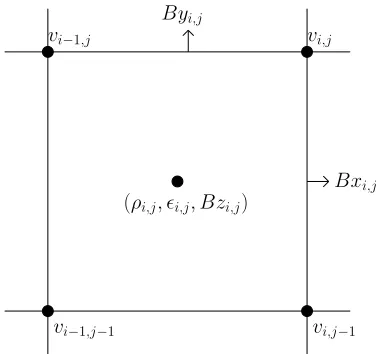
[image:37.612.218.406.214.391.2](ρi,"i)
Fig. 2.1: Position of variables defined on a 1D grid.
(ρi,j,"i,j, Bzi,j)
vi−1,j vi,j
vi,j−1
Bxi,j
Byi,j
vi−1,j−1
Fig. 2.2: Position of variables defined on a 2D grid.
Bz vz
By
(ρ,")
vy vx
Bx
[image:37.612.216.412.460.631.2]2.3 The LareXd Code 24
The volume of each cell is not necessarily constant as an additional feature ofLareXdis that the grid can be stretched in any of the spatial directions. For this thesis, however, this option is not used.
Using similar notation as Arber et al. (2001), we note that the averaging used depends on whether the variable is a volume average, like the density, or a surface average, like the magnetic field. We also define
xci,j,k,yci,j,kandzci,j,kas the cell centres in thex,yandz directions andxbi,j,k,ybi,j,kandzbi,j,kas
the cell boundaries in thex,yandzdirections.dxci,j,k,dyci,j,kanddzci,j,kare the distances between cell
centres anddxbi,j,k,dybi,j,kanddzbi,j,kare the lengths of the cell in thex,yandzdirections. Note that
the boundary position is the same as the cell centre position plus half of the length of the cell, i.e.
xbi,j,k = xci,j,k+dxbi,j,k/2,
ybi,j,k = yci,j,k+dybi,j,k/2,
zbi,j,k = zci,j,k+dzbi,j,k/2.
The density, internal energy density and the plasma pressure areρi,j,k,#i,j,kandpi,j,k, respectively, and
are defined at the cell volume centre at(xc, yc, zc)i,j,k.
The magnetic field components are each defined at different locations.Bxi,j,kis defined at the centre of
the right boundary,(xb, yc, zc)i,j,k. Byi,j,kis defined at the centre of the back boundary,(xc, yb, zc)i,j,k
andBzi,j,kis defined at the centre of the top boundary,(xc, yc, zb)i,j,k.
The velocity components,vxi,j,k,vyi,j,k andvzi,j,k are all defined at the top, right back vertex, i.e.
(xb, yb, zb)i,j,k.
To obtain the density at the cell vertex,ρv
i,j,k, control volume averaging is used (for more details, see
Arber et al. (2001)). The magnetic field components at the cell centre are simply the averages of the values on opposing faces. The velocity components defined on cell faces, e.g. vxbi,j,kare found by averaging
over the four vertex values.
2.3.2 Lagrangian Step
The Lagrangian step is a straight forward predictor-corrector scheme, where predicted values are calculated from an Eulerian step with time stepdt/2, and then corrected at the full time stepdt. Conservation of mass is then used to simplify the time-centered Lagrangian terms by evaluating derivatives on the original Eulerian grid. The end result is a second order scheme in time and space which is fully 3D and does not use conservative form.
2.3 The LareXd Code 25
Dρ Dt +ρ
∂v
∂x= 0, (2.10)
Dv Dt +
1
ρ ∂p
∂x = 0, (2.11)
D# Dt +
p ρ
∂v
∂x= 0, (2.12)
where D
Dt = ∂ ∂t +v
∂
∂x= 0is the convective derivative.
Solving in Lagrangian form means that the grid will move with the fluid and become distorted from the original Eulerian configuration. Ifdxbiis the distance between boundaries for cellianddxciis the distance
between cell centres, then after one time stepdt, Eq. (2.9) implies that the change in the cell volume of cell
iis,
∆=dxbi+ (v
n+1/2
i −v n+1/2
i−1 )dt
dxbi
,
where the time centred velocityvn+1/2has been used to make∆second order accurate in time.
Since mass is conserved in a cell from one time step to the next, the new density is simply
ρni+1=
ρn i
∆.
From the new grid all other variables can be found from the change in volume/shape of the grid.
The spatial differencing used is second order accurate as derivatives are always centred on a staggered grid. For example we have
&
dp dx
'
cell boundary
=pi+1−pi
dxci
2.3 The LareXd Code 26 & dv dx ' cell centre
=vi−vi−1
dxbi
.
Predictor step
The grid is evaluated at the half time step as
dxbni+1/2=dxbn i +
1 2dt(v
n
i −vni−1).
The 1D Euler equations, Eq. (2.10)-Eq. (2.12), then give us the velocity, the energy density and the pressure at the half time step as
#ni+1/2−#n i
dt/2 =−p
n i
vn i −vin−1
ρn idxbni
,
vin+1−vn i
dt/2 =
−pn i+1−pni
ρn
i+1/2dxcni
,
pni+1/2=# n+1/2
i (γ−1)ρ n+1/2
i
dxbn i
dxbni+1/2
.
Corrector step
The update for the velocity can now be found,
vin+1−vn i
dt = −
pni+1+1/2−p
n+1/2
i
ρni+1+1//22dxcni+1/2
= −p
n+1/2
i+1 −p
n+1/2
i
ρn
i+1/2dxcni
,
since mass is conserved, it has the same value as at time stepn, i.e.,ρin+1+1//22dxcni+1/2=ρn
2.3 The LareXd Code 27
means that all derivatives can be taken on the original Eulerian grid.
Asvis defined at the boundary we need to averageρto find its value at the boundary. So we have
ρi+1/2=
dxbiρi+dxbi+1ρi+1
2dxci .
For the velocity at the half-time step we simply use
vin+1/2=
1 2(v
n
i +vin+1).
The updated energy can now be found from,
#ni+1−#n i
dt =−p
n+1/2
i
vni+1/2−v n+1/2
i−1
ρn idxbni
.
All that remains is to update the grid and find the new density. Hence,
dxbni+1=dxbn i +dt(v
n+1/2
i −v n+1/2
i−1 )
and
ρni+1=ρni
dxbn i
dxbni+1.
The 1D Euler equations have now evolved one time step.
2.3.3
The Remap Step
At the end of the Lagrangian step all the variables have been updated on a grid that has moved with the fluid. These variables now need to be remapped back onto the original Eulerian grid. This process is a geometrical step, designed to maintain monotonicity.
2.4 Summary 28
2.3.4 Using the Code
To use the code we must set up our initial conditions, i.e. set the magnetic field components, velocity components, density and specific internal energy density. We also specify how these variables behave at the boundaries of the domain. Lastly, the control file allows us to set the grid resolution, time step, resistivity, viscosity and other such parameters.