Solution of Boundary-Value Problems using Kantorovich Method
A.A. Gusev1,a, L.L. Hai1,2, O. Chuluunbaatar1,3, S.I. Vinitsky1,b, and V.L. Derbov4
1Joint Institute for Nuclear Research, Dubna, Russia, 2Belgorod State University, Belgorod, Russia
3National University of Mongolia, UlaanBaatar, Mongolia 4Saratov State University, Saratov, Russia
Abstract. We propose a computational scheme for solving the eigenvalue problem for an elliptic differential equation in a two-dimensional domain with Dirichlet boundary con-ditions. The solution is sought in the form of Kantorovich expansion over the basis func-tions of one of the independent variables with the second variable treated as a parameter. The basis functions are calculated as solutions of the parametric eigenvalue problem for an ordinary second-order differential equation. As a result, the initial problem is reduced to a boundary-value problem for a set of self-adjoint second-order differential equations for functions of the second independent variable. The discrete formulation of the problem is implemented using the finite element method with Hermite interpolation polynomials. The efficiency of the calculation scheme is shown by benchmark calculations for a square membrane with a degenerate spectrum.
1 Introduction
The calculation of spectral and optical properties of electronic states in axially symmetric quantum dots is reduced to the solution of two-dimensional boundary-value problems (BVP) for elliptic differ-ential equations with nonseparable variables in a finite domain [1]. One of the ways to solve these problems is implemented as the set of programs ODPEVP-KANTBP [2, 3] based on the Kantorovich method that provides the reduction of the initial problem to a set of ordinary differential equations [4] with further use of the finite element method [5] with Lagrange interpolating polynomials. For the impurity states of quantum dots such BVPs are defined in domains of complicated geometry and involve piecewise-continuous potential functions. In this case it is necessary to preserve not only the continuity of the approximate solution, but also the continuity of its first derivative, which is most naturally achieved using the finite element method with Hermite interpolating polynomials [6, 7].
Testing such approach for the solution of two-dimensional BVPs is the aim of the present work. We present a computational scheme for solving the eigenvalue problem for an elliptic differential equation in a two-dimensional finite domain with Dirichlet boundary conditions. The solution is sought in the form of Kantorovich expansion over the basis functions of one of the independent vari-ables with the second variable treated as a parameter. The basis functions are calculated as a solution
of the parametric eigenvalue problem for an ordinary second-order differential equation. Finally, the
initial problem is reduced to a BVP for a set of self-adjoint second-order differential equations for
functions of the second independent variable. The discretization of the problems is carried out using the finite element method with Hermite interpolation polynomials.
The result is used to formulate a generalized algebraic eigenvalue problem. For matrices of small dimension this problem is solved using Maple. For matrices of large dimension we use the symbolic algorithm to generate Fortran routines for numerical solution of the generalized algebraic eigenvalue
problem. We demonstrate the efficiency of the programs generated in Maple and Fortran for 100×100
and higher-order matrices, respectively, in benchmark calculations for the exactly solvable eigenvalue problem of a square membrane with degenerate spectrum. This example is not trivial from the com-putational view point. It shows the applicability of the method, algorithms and program in solving the generalized algebraic eigenvalue problem with the higher-order matrices which has a quasidegen-erate spectrum. The use of new coordinates that can be separated within the domain but not at the boundary allows the simulation of a potential function, depending upon two variables, and justifies the application of the Kantorovich method.
2 Kantorovich Method
Let us consider the 2D BVP in the two-dimensional domainΩ(xf,xs)⊂R2:
−∂∂2 xs −
∂2
∂xf +
V(xf,xs)−E
Ψ(xf,xs)=0, (1)
whereV(xf,xs) is a real-valued function andΨ(xf,xs) satisfies the Dirichlet condition at the boundary
∂Ω(xf,xs) of the domainΩ(xf,xs)
Ψ(xf,xs)
(xf,xs)∈∂Ω(xf,xs)=
0. (2)
The solutionΨ(xf,xs)∈W22(Ω) of the BVP (1)–(2) is sought as a Kantorovich expansion [4]
Ψv(xf,xs)= jmax
j=1
Φj(xf;xs)χjv(xs) (3)
over the set of eigenfunctionsΦj(xf;xs)∈ Fxs ∼W22(Ωxf(xs)) of the parametric BVP
−∂∂2 xf +
V(xf,xs)−j(xs)
Φ(xf;xs)=0, (4)
defined in the intervalxf ∈(xminf (xs),xmaxf (xs))= Ωxf(xs) and depending on the variablexs∈Ωxsas a
parameter. These functions obey the boundary conditions
Φj(xminf (xs);xs)=0, Φj(xmaxf (xs);xs)=0 (5)
at the boundary points{xmin
f (xs),x
max
f (xs)} = ∂Ωxf(xs), of the interval Ωxf(xs). The eigenfunctions
satisfy the orthonormality condition in the same intervalxf ∈Ωxf(xs):
Φi|Φj
=
xmax
f (xs)
xmin
f (xs)
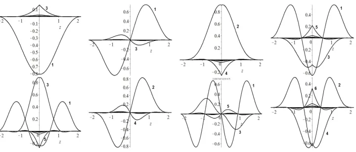
Figure 1.The componentsχjv(xs) of the Kantorovich expansion (3) corresponding to the first eight eigenvalues
Here1(xs)<· · ·< jmax(xs)<· · · is the desired set of real eigenvalues. If this parametric eigenvalue problem has no analytical solution, then it is solved numerically using the program ODPEVP [2].
Substituting (3) into (1) with (5) and (6) taken into account, we arrive at the set of self-adjoint ODEs for the unknown vector functionsχv(xs,E)≡χv(xs)=(χ1v(xs), . . . , χjmaxv(xs))
T ∈W2 2(Ωxs):
−Id2
dx2
s
+U(xs)−2EvI+dQdx(xs)
s +
Q(xs)
d dxs
χv(xs)=0. (7)
HereU(xs) andQ(xs) are matrices of the dimension jmax×jmax
Ui j(xs)=i(xs)δi j+Hi j(xs),
Hi j(xs)=Hji(xs)= xmax
f (xs)
xmin
f (xs)
∂Φi(xf;xs)
∂xs
∂Φj(xf;xs)
∂xs
dxf, (8)
Qi j(xs)=−Qji(xs)=− xmax
f (xs)
xmin
f (xs)
Φi(xf;xs)
∂Φj(xf;xs)
∂xs
dxf.
The discrete spectrum solutionsE:E1<E2<· · ·<Ev <· · · that obey the boundary conditions
at the pointsxt
s={xmins ,xsmax}=∂Ωxslocated at the boundary ofΩxsand the orthonormality conditions χv(xts)=0, xts=xmin
s ,xmaxs ,
xmax
s
xmin
s
(χv(xs))Tχv(xs)dxs=δvv (9)
are calculated by means of the program KANTBP [3].
3 Benchmark calculation: rectangular membrane
As a benchmark example we consider the exactly solvable BVP for a rectangular membrane in con-ventional variables (x, y)∈Ω(x, y)
−∂2 ∂x2 −
∂2
∂y2 −E
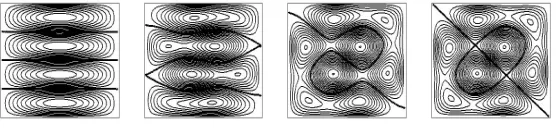
Figure 2. Profiles of the linear combinations of the eigenfunctionsΨ2(xf,xs) andΨ3(xf,xs) corresponding to
linear combinations of exact solutionsu12andu21:u12,u12+
√
2/3u21,u12+u21
Figure 3.Profiles of the linear combinations of the eigenfunctionsΨ5(xf,xs) andΨ6(xf,xs) corresponding to the linear combinations of the exact solutionsu13andu31:u13+u31,u13+(1/3)u31,u13,u13−(2/3)u31,u13−u31
Figure 4. Profiles of the linear combinations of the eigenfunctionsΨ7(xf,xs) andΨ8(xf,xs), corresponding to
the linear combinations of the exact solutionsu23andu32:u23,u23+(1/3)u32,u23+u32
Figure 5. Profiles of the linear combinations of the eigenfunctionsΨ9(xf,xs) andΨ10(xf,xs) corresponding to
the linear combinations of the exact solutionsu14andu41:u14,u14+(1/3)
√
2/3u41,u14+
√
2/3u41,u14+u41
with the Dirichlet conditions forΨ(x, y) at the boundary∂Ω(x, y) of the regionΩ(x, y)
Ψ(±a/2, y)=0, Ψ(x,±b/2)=0. (11)
We solve the BVP (1)–(2) for the rectangular membranex∈(−a/2,a/2),y∈(−b/2,b/2), in the new variables xf=(x+y)/
√
2, xs=(x−y)/
√
2 withV(xf,xs)=0. The new variables can be separated
withinΩbut not at the boundary∂Ω, which simulates the presence of a potentialV(xf,xs)0 and
eigenfunctionsΦi xf;xs
and the potential curvesi(xs) are expressed in the analytical form
i(xs)= π
2i2
(xmax
f (xs)−xminf (xs))2
, Φi xf;xs = √ 2 sin ⎛ ⎜⎜⎜⎜⎜ ⎝ π
i(xf−xminf (xs))
xmax
f (xs)−xminf (xs) ⎞ ⎟⎟⎟⎟⎟ ⎠
xmax
f (xs)−xminf (xs)
. (12)
With the basis functions (12), the integration in the effective potentials (8) can be carried out analyti-cally. This yields the expressions
Qi j(xs)=−
2i j i2−j2
⎛ ⎜⎜⎜⎜⎜
⎝(−1)i+jdx
max
f (xs)
dxs −
dxmin
f (xs)
dxs ⎞ ⎟⎟⎟⎟⎟ ⎠
xmax
f (xs)−xminf (xs)
, ji,
Hi j(xs)=−
4i j(i2+j2)
(i2−j2)2
⎛ ⎜⎜⎜⎜⎜
⎝(−1)i+jdx
max
f (xs)
dxs
−dx
min
f (xs)
dxs ⎞ ⎟⎟⎟⎟⎟ ⎠ ⎛ ⎜⎜⎜⎜⎜ ⎝dx max
f (xs)
dxs
−dx
min
f (xs)
dxs ⎞ ⎟⎟⎟⎟⎟ ⎠
(xmax
f (xs)−xminf (xs))2
, (13)
Hii(xs)= π
2i2
3
⎛ ⎜⎜⎜⎜⎝dxmax
f (xs)
dxs ⎞ ⎟⎟⎟⎟⎠2
+
⎛ ⎜⎜⎜⎜⎝dxmax
f (xs)
dxs ⎞ ⎟⎟⎟⎟⎠⎛⎜⎜⎜⎜⎜⎝dxmin
f (xs)
dxs ⎞ ⎟⎟⎟⎟⎟ ⎠+ ⎛ ⎜⎜⎜⎜⎜ ⎝dx min
f (xs)
dxs ⎞ ⎟⎟⎟⎟⎟ ⎠ 2 (xmax
f (xs)−xminf (xs))2
+1 4 ⎛ ⎜⎜⎜⎜⎜ ⎝ dxmax
f (xs)
dxs −
dxmin
f (xs)
dxs ⎞ ⎟⎟⎟⎟⎟ ⎠ 2 (xmax
f (xs)−x
min
f (xs))2
.
In the symmetric casea=b: xmax
f (xs)=−x
min
f (xs) the matrix elementsHi jandQi jbetween even
and odd indexes equal zero and one can solve the BVP for even (e) and odd (o) solutions separately.
Numerical calculations of the eigenvalue problem (7)–(9) were carried out for jmax=6 using the
program KANTBP4M implemented in Maple on the gridΩxs =(−xm(4)−7xm/8(4)0(4)7xm/8(4)xm) at
xm=π/
√
2−1/20, where the number of finite elements in each subinterval is presented in parentheses.
The finite-element local functions are constructed using the Hermite interpolation polynomials of the seventh order (p=κmax(p+1)−1=7) with the multiplicity of the nodesκmax
r =1 andp+1=8 in each
of the elements [7], which provides the accuracyO(hp+1) of the eigenfunctions and the eigenvalues,
wherehis the maximal element length. The dimension of the mass and stiffness matrices is 666×666
and their half-width is 48. The componentsχjv(xs) of the corresponding eigenfunctionsΨv(xf,xs) are
shown in Fig. 1 that allows one to estimate the accuracy of the Kantorovich expansion (3) to be of
the order of 4·10−4÷10−2 and the accuracy of the corresponding eigenvaluesEσ
v: 2.0004, 5.0004,
5.0017, 8.0050, 10.0042, 10.0016, 13.0034, 13.0153, 17.0050, 17.0053 of the order 4·10−4÷10−2,
in comparison with the exact valuesEv: 2, 5, 5, 8, 10, 10, 13, 13, 17, 17. For the number jmax of
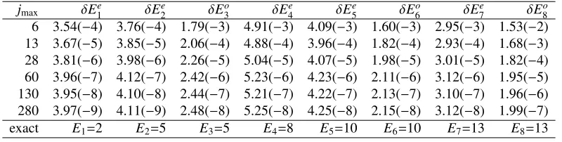
the parametric basis functions increased to 280, more RAM and computer time are needed. Here,
we used the Fortran version of the program KANTBP4, which provides the accuracyO(hp+1) of
the eigenfunctions andO(h2p) of the eigenvalues, and achieved the discrepancyδEσ
v = Evσ−Ev
of the order of 10−8 for the eigenvalues that is shown in Table 1. One can see from the Table that
the convergence rate of the Kantorovich expansion (3) is the order of j−3
max which corresponds to the
Table 1.The discrepancyδEσv =Eσv −Ev,σ=e,ovs a number of even (e) and odd (o) basis functionsjmax
jmax δE1e δE2e δEo3 δE4e δE5e δE6o δE7e δE8o
6 3.54(−4) 3.76(−4) 1.79(−3) 4.91(−3) 4.09(−3) 1.60(−3) 2.95(−3) 1.53(−2) 13 3.67(−5) 3.85(−5) 2.06(−4) 4.88(−4) 3.96(−4) 1.82(−4) 2.93(−4) 1.68(−3) 28 3.81(−6) 3.98(−6) 2.26(−5) 5.04(−5) 4.07(−5) 1.98(−5) 3.01(−5) 1.82(−4) 60 3.96(−7) 4.12(−7) 2.42(−6) 5.23(−6) 4.23(−6) 2.11(−6) 3.12(−6) 1.95(−5) 130 3.95(−8) 4.10(−8) 2.44(−7) 5.21(−7) 4.22(−7) 2.13(−7) 3.10(−7) 1.96(−6) 280 3.97(−9) 4.11(−9) 2.48(−8) 5.25(−8) 4.25(−8) 2.15(−8) 3.12(−8) 1.99(−7)
exact E1=2 E2=5 E3=5 E4=8 E5=10 E6=10 E7=13 E8=13
The calculation time was about 100 sec. forjmax=6 in Maple and 80 sec. for jmax=60 in Fortran
using a PC Intel Core i5 3.33GHz, 4Gb RAM, and a 64 bit Windows 7 as the operation system. It is known that the eigenvalues of the rectangular membrane BVP may be degenerate. It is
always the case, if the aspect ratioa : b is a rational number, because in this case the equation
m2/a2+n2/b2=m2/a2+n2/b2always has nontrivial integer solutions. For example, in the present
case of a square membrane witha = b = πsuch a solution ism = n,n = m. For the boundary
conditionu = 0 the corresponding fundamental functions are sinmxsinny and sinnxsinmy. For
any eigenvalue the degeneracy order is determined by the solution of the number theory problem of
how many ways exist to represent an integerν2 as a sum of two squares: ν2 = m2+n2 The nodal
lines for the eigenfunctions sinnxsinmyare just straight lines parallel to the coordinate axes (x, y). However, with degenerate eigenvalues quite different nodal lines may appear, e.g., the square has
a locus of points at which the functionαsinnxsinmy+βsinmxsinnyequals zero. In Figs. 2–5
some typical examples of profiles and nodal lines of linear combinations of the eigenfunctions are presented, corresponding to the exact doubly degenerate eigenvalues 5, 10, 13, and 17. In the captions
the notationumn = sinmxsinnyis used. The nodal lines of the eigenfunctions are shown by solid
curves, which coincide with those presented in [8].
Acknowledgements
The authors thank Prof. V.P. Gerdt for collaboration and support of this work. The work was partially supported by the Russian Foundation for Basic Research (RFBR) (grants Nos. 14-01-00420 and 13-01-00668) and Hulubei-Meshcheryakov Program JINR-Romania, JINR Order 33/23.02.2015, p. 98.
References
[1] A.A. Gusev et al, Lect. Notes Comput. Sci.6244, 106–122 (2010)
[2] O. Chuluunbaatar et al, Comput. Phys. Commun.180, 1358–1375 (2009)
[3] O. Chuluunbaatar et al, Comput. Phys. Commun.179, 685–693 (2008)
[4] L.V. Kantorovich, V.I. Krylov,Approximate Methods of Higher Analysis(Wiley, New York, 1964)
[5] G. Strang, G.J. Fix,An Analysis of the Finite Element Method(Prentice-Hall, Englewood Cliffs,
New York, 1973)
[6] L. Ramdas Ram-Mohan,Finite Element and Boundary Element Aplications in Quantum
Mechan-ics, (Oxford University Press, New York, 2002)
[7] A.A. Gusev et al, Lect. Notes Comput. Sci.8660, 140–156 (2014)
[8] R. Courant, D. Hilbert,Methods of Mathematical Physics. Vol. 1(John Wiley & Sons, New York,