YAN, JIAHONG. Development and Implementation of a Time-of-Use Based Home Energy Management System. (Under the direction of Dr. Ning Lu).
Power system is experiencing rapid change on both supply and demand side. The
increasing renewable generation, such as solar and wind generation, cause more variation of
power supply and operation uncertainty, while the behind-meter solar and transportation
electrification are reshaping the end-use demand curve. Such a change brings system operators a
challenge to balance the system reliably and economically. On the other hand, load service
entities are implementing time-varying electricity price to reflect the true cost of generation in a
day, and energy consumers need to use energy accordingly. Thus, both system operators and
energy consumers are seeking a tool to resolve the new problem raised by new trend in power
system. In this dissertation, I focus on developing and implementing an Home Energy
Management System (HEMS) with an objective to save residential costumers’ energy cost and
improve the energy demand curve for the power system.
Chapter 2 reviews the current technologies in HEM, and proposes a prototype of HEMS
with both software and hardware design. A physical test system and graphical-user-interface of
HEM is designed and implemented at FREEDM Center of North Carolina State University
(NCSU). A demonstration case shows the functionalities and capability of an HEMS.
As an essential component in HEM, the household energy demand forecast is studied in
Chapter 3. The proposed forecaster provides both day-ahead and hour-ahead demand forecast for
HEMS. Considering the high volatility and randomness of house-level energy demand,
progressive technologies are used to forecast the demand in both probabilistic and deterministic
ways. In day-ahead, similar days are grouped based on the weather and “day of week”
updates a state-space model to provide point estimate of hour-ahead load. Case study with 20
realistic house energy demand data show the effectiveness of the proposed forecasting approach.
Another core component of HEM is the scheduling algorithm. In chapter 4, controllable
appliances are categorized in three main types and modeled according to their physical features.
Instead of using mathematical optimization approach, the propose scheduling algorithm
schedules smart load in a heuristic way based on different model types, such that it is
computational effective and robust to demand forecast uncertainty. More important, the proposed
HEM considers users’ comfort preference and the cost saving expectation. A mechanism is
developed to quantify users’ cost saving expectation in return of comfort setting sacrifice. A case
study shows the cost saving and load profile improvement are achieved by the proposed HEM.
In Chapter 5 of the dissertation, the aggregate impact of HEM is discussed. The main
problem for high penetration HEM is the “loss of load diversity” issue. A control strategy is
proposed to mitigate such an issue by introducing an artificial randomness in each individual
HEMS. A case study with IEEE 123-node feeder system shows how the mitigation approach
improve the system reliability and efficient. In addition, Chapter 5 discusses how the proposed
HEMS can map the household-level smart appliance to demand response in wholesale energy
market. A three-bus system example shows the aggregate HEM can relieve transmission
© Copyright 2018 by Jiahong Yan
by Jiahong Yan
A dissertation submitted to the Graduate Faculty of North Carolina State University
in partial fulfillment of the requirements for the degree of
Doctor of Philosophy
Electrical Engineering
Raleigh, North Carolina
2018
APPROVED BY:
_______________________________ _______________________________ Dr. Ning Lu Dr. David Lubkeman
Committee Chair
_______________________________ _______________________________
ii
DEDICATION
iii
BIOGRAPHY
Jiahong Yan was born in Guangdong, China. He received his B.S. degree in electrical
engineering from South China University of Technology, Guangzhou, China in 2010, and his
M.S. degree in electrical engineering from Tianjin University, Tianjin, China in 2013. He is
currently pursuing the Ph.D. degree in electrical engineering at North Carolina State University,
Raleigh, NC. His current research interests include home energy management system, energy
iv
ACKNOWLEDGMENTS
My foremost and deepest gratitude goes to my advisor, Prof. Ning Lu, for her continual
support, encouragement, and guidance. Prof. Lu is my advisor, not only in academic study, but
also in career and life. She provides me great opportunities of becoming a good researcher and
encourages me to pursue my dream and work on the area I am interested in. She is always a role
model for me to be passionate in research, educating and life. I am so grateful to Prof. Lu for her
invaluable advice on my research, career development, presentation, technical writing, and many
other aspects that are priceless fortune to me.
My great appreciation and thankfulness also goes to my committee members: Prof. David
Lubkeman, Prof. Srdjan Lukic, and Prof. Eric Chi, for their precious time and help. Their passion
on research always motivated me to devote myself to my research and the exploration to the new
areas.
I wish to thank many great lab mates in my life, I would like to express my sincere thanks
to them: Xiangqi Zhu, Jiyu Wang, Xinda Ke,Jian Lu, Gonzague Henri, David Mulcahy,
Weifeng Li, Fuhong Xie, Ming Liang and Lining Dong. All of the great memories with them are
indispensable parts of my life.
Last, but surely not the least, I would like to thank my family for their love and support.
They always encourage me to chase my dream and provide me the opportunity to be the person I
want to be. Nobody is more important to me in the pursuit of the PhD than my wife Dr. Cuiyan
Kong, whose continued and unfailing love and support are always with me in the past thirteen
years. We share the happiness and sadness in our life and throughout the pursuit of our PhDs. To
my beloved daughter Keira Yan, I would like to express my thanks for being such a good girl
v
TABLE OF CONTENTS
LIST OF TABLES ... vii
LIST OF FIGURES ... viii
CHAPTER 1 INTRODUCTION ...1
1.1 An Overview of Demand Side Management Methods ... 1
1.2 Home Energy Management System... 3
1.3 Technical Challenges ... 5
1.4 Overview of Thesis Framework... 7
1.5 Contributions of the Thesis ... 9
1.6 Organization of the Thesis ... 11
CHAPTER 2 DESIGN OF HOME ENERGY MANAGEMENT SYSTEMS ...12
2.1 Background ... 12
2.2 Optimization Objectives and Key Functionalities of the HEM System ... 13
2.3 The Proposed Hardware Prototype ... 15
2.3.1 HEM Controller ... 16
2.3.2 Smart Switch and Smart Thermostat ... 17
2.3.3 HEM Communication Network ... 17
2.4 The Proposed Software Architecture ... 19
2.4.1 Software Layers and Interfaces ... 19
2.4.2 HEM Information Flow ... 21
2.4.3 HEM Algorithms Overview ... 22
2.5 HEM Testing System Implementation... 24
2.5.1 HEM Hardware Testbed ... 25
2.5.2 Graphical User Interface ... 26
2.5.3 A Demonstration Case of HEM Testing System ... 28
CHAPTER 3 A HOUSEHOLD ELECTRICITY LOAD FORECAST APPROACH FOR HOME ENERGY MANAGEMENT SYSTEM ...33
3.1 Introduction ... 33
3.2 Methodology ... 35
3.2.1 Day-ahead load level probabilistic forecast ... 36
3.2.2 Hour ahead load forecast with Kalman filter ... 42
vi
3.3.1 Data preparation ... 46
3.3.2 Accuracy Measurement ... 47
3.3.3 Results ... 50
3.4 Summary ... 59
CHAPTER 4 LOAD MODELING AND CONTROL STRATEGRY FOR HEMS WITH HEURISTIC APPROACH UNDER TIME-OF-USE PRICING ...61
4.1 Introduction ... 61
4.2 Controllable Load Modeling ... 63
4.2.1 TCA Modeling ... 64
4.2.2 TBA Modeling ... 67
4.2.3 EV Modeling ... 69
4.3 Control Strategy ... 70
4.3.1 TCA Control Strategy ... 71
4.3.2 TBA Control Strategy ... 74
4.3.3 EV Control Strategy ... 76
4.3.4 Power-Cap Control Strategy ... 80
4.4 Case study ... 82
4.4.1 Case description ... 82
4.4.2 Results ... 84
4.4.3 Discussion ... 87
4.5 Summary ... 90
CHAPTER 5 AGGREGATE STUDY OF HOME ENERGY MANAGEMENT ...92
5.1 Introduction ... 92
5.2 High HEMS Penetration on Distribution Feeder: Problem and Mitigation ... 94
5.2.1 Problem of High HEMS Penetration ... 94
5.2.2 Control Strategy of Mitigating “Loss of Load” ... 97
5.3 HEM Demand Response in Wholesale Market ... 100
5.3.1 Mapping End-user Comfort Setting to DR Bidding ... 100
5.3.2 Example: A Three-bus System with HEMS DR ... 102
5.4 Summary ... 104
CHAPTER 6 CONCLUSION ...105
vii
LIST OF TABLES
Table 2.1 Appliances setting ... 30
Table 3.1 DA forecast error of 20 houses in 2 summer and winter weeks ... 55
Table 3.2 AMAPE of HA forecast for summer and winter case ... 58
Table 4.1 Controllable appliances setting ... 83
Table 4.2 Simulation results summary... 87
Table 4.3 Power cap level impact on user’s comfortableness ... 90
Table 5.1 System average daily loss ... 95
viii
LIST OF FIGURES
Figure 1.1 CAISO's 2013 illustration of the “duck curve” ...2
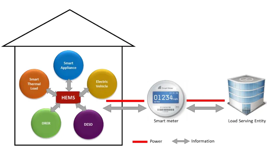
Figure 1.2 Smart house schematic diagram ...4
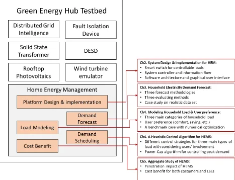
Figure 1.3 GEH research project framework ...8
Figure 2.1 Lifecycle of an HEM Operation Forming the OODA Loop ...14
Figure 2.2 HEM hardware system overview ...16
Figure 2.3 Mesh ZigBee network topology of HEM ...18
Figure 2.4 HEM software framework ...19
Figure 2.5 Information flow among smart device, local and cloud controller ...22
Figure 2.6 Timeline of forecasting and scheduling algorithm horizon and update frequency ....23
Figure 2.7 1-SST Test System Schematic Diagram ...24
Figure 2.8 Physical HEM testbed in FREEDM System Center ...25
Figure 2.9 Smart switch diagram ...26
Figure 2.10 A Matlab-based Graphical User Interface ...27
Figure 2.11 Case setting (a) TOU price curve, (b) base-load ...29
Figure 2.12 Demonstration case results ...31
Figure 2.13 Voltage and Power at the SST side ...32
Figure 3.1 Household electricity load forecast process: DA and HA ...36
Figure 3.2 A household load and temperature daily change ...37
Figure 3.3 An example of sorted household load ...40
Figure 3.4 Data structure for multinomial logistic regression ...41
Figure 3.5 Moving window of data points selected in the load forecast model ...44
Figure 3.6 State-space Kalman filter algorithm flowchart ...46
Figure 3.7 Illustration of probabilistic forecast error triangle ...48
Figure 3.8 DB index of different cluster numbers in different months ...50
Figure 3.9 Average Weather in Austin, TX [92] ...51
Figure 3.10 An August forecasted day cluster results of daily temperature ...51
Figure 3.11 A February forecasted day cluster results of daily temperature ...51
Figure 3.12 DA probabilistic forecast result for one house on Aug.31, 2016 ...53
Figure 3.13 Actual load and selected thresholds for one house on Aug.31, 2016 ...53
Figure 3.14 DA forecast error for one house on Aug.31, 2016 ...53
ix
Figure 3.16 Actual load and selected thresholds for one house on Dec. 22, 2016 ...54
Figure 3.17 DA forecast error for one house on Dec. 22, 2016 ...54
Figure 3.18 A moving window of selected point in HA model ...56
Figure 3.19 HA forecast of a house load in a summer day ...56
Figure 3.20 WMAE of HA forecast of a house load in a summer day ...57
Figure 3.21 HA forecast of a house load in a winter day ...57
Figure 3.22 WMAE of HA forecast of a house load in a winter day ...58
Figure 4.1 A typical thermal characteristic curve of an electric water heater load ...64
Figure 4.2 An example of the TCA status and switch on/off indicators ...66
Figure 4.3 A mechanism for HEMS to extend the setpoint according to user’s cost saving expectation ...72
Figure 4.4 Algorithm flowchart of HEMS TCA control strategy (cooling mode) ...73
Figure 4.5 A mechanism for HEMS to delay TBA task according to user’s cost saving expectation ...75
Figure 4.6 Algorithm flowchart of HEMS TBA control strategy ...76
Figure 4.7 EV charging time and charge rates based on price and available time ...77
Figure 4.8 A mechanism for HEMS to adjust SoC target according to user’s cost saving expectation ...78
Figure 4.9 Algorithm flowchart of HEMS EV charging control strategy ...79
Figure 4.10 A rolling priority list for selecting appliance to turn off ...81
Figure 4.11 Algorithm flowchart of HEMS power cap control strategy ...82
Figure 4.12 TOU price and outdoor temperature used in the case study ...83
Figure 4.13 DA probabilistic load forecast in the case study ...84
Figure 4.14 Household total energy usage comparison with and without HEMS ...85
Figure 4.15 Air conditioner energy usage and temperature comparison with and without HEMS ...85
Figure 4.16 Water heater energy usage and temperature comparison with and without HEMS ...86
Figure 4.17 TBAs energy usage comparison with and without HEMS ...86
Figure 4.18 EV charging and SoC comparison with and without HEMS ...87
Figure 5.1 Substation level load profiles under different HEMS penetrations ...94
Figure 5.2 IEEE 123-node test feeder used in the HEMS aggregate study ...95
Figure 5.3 Voltage profiles at some selected nodes ...96
x Figure 5.5 An illustration of “random off-peak start time” based on comfort condition
priority ...98
Figure 5.6 Comparison of total load profiles with three control strategies to mitigate “loss of load diversity” issue ...99
Figure 5.7 Voltage profile at some selected nodes before and after “loss of load diversity” mitigation ...100
Figure 5.8 Three-bus system example ...102
Figure 5.9 LMP and dispatch results with Line B-C congested ...103
1
CHAPTER 1 INTRODUCTION
This chapter introduces the state-of-the-art of demand side management technologies,
presents the technical challenges, and summarizes the main contribution of the thesis.
1.1
An Overview of Demand Side Management MethodsTraditionally, power systems operation applies a centralized, top-down approach.
Electricity is generated by large, MW-level power plants. Power flows are normally
one-directional in power distribution grid: from substations to the loads. In the past ten years,
renewable generation resources are rapidly integrated to the grid from both the transmission and
distribution level, causing significant increase in power variations and uncertainties in grid
operation [1]. Furthermore, behind meter solar and the rapidly adoption of electrical vehicles are
causing shifts in residential and commercial load patterns [2, 3]. The famous California daily
“duck curve” illustrates the drastic change in daily load profiles at regional level caused by the
increase in solar generation across the state. As shown in Figure 1.1, a deep valley is formed in
the middle of the day. This causes a sharp decrease of energy consumption after the solar
generation picks up the load in the morning right after a steep increase to the morning peak in the
early evening (7 – 9 p.m.). This curve is not unique to California. Many grid operators in areas
with high solar penetration feeders start to observe such load patterns.
The “duck curve” brings two main issues to the power system operators and planners:
maintain enough conventional generation capacity to supply peak load while solar generation is
not available and maintain enough flexible ramping resources to follow the variations caused by
2
Figure 1.1 CAISO's 2013 illustration of the “duck curve”[4]
Demand Side Management (DSM) is the demand side solutions to alleviate the power
system stress of energy balancing. Main DSM applications include load shifting [5], peak
shaving [6], load following [7], frequency response [8], and smoothing of intermittent generation
resources [9] using distributed energy resources such as energy storage, distributed generators,
electric vehicles, or controllable loads. Traditionally, DSM was mainly used for peaking shaving
and load shifting for hedging price spikes, investment deferral, or low-frequency load shedding
[10]. In recent years, there are some new trends in DSM due to the smart grid initiative and new
pricing schemes in electricity market operation:
• Using the data collected in DSM programs for advanced data analytics such as load
forecast, end use pattern detection, nonintrusive load monitoring, fault detection, etc.
• Accurate real-time load control. The reduction in the cost of wireless communication
makes it affordable for more accurate real-time load control via smart meters or smart
3 • Time-varying retail prices are implemented by the Load Serving Entities (LSE) to
reflect the wholesale electricity market (if applicable) price dynamic or system status.
It requires intelligent DSM to help energy consumers to adjust their demand patterns
accordingly.
• The DSM promotes the distributed generation consumed locally, deferring new
transmission line expansion or reducing energy storage requirement.
• In the past, the DSM is mainly “utility driven”, it moves towards “customer driven” in
the future.
These new trends in the DSM draws increasing attention from both research and industry
on developing advance energy management systems for energy consumers, especially for
residential consumers. According to U.S. Energy Information Administration (EIA), the
residential electricity use in U.S. is over one third of the total electricity use [11], which is the
largest share sector. The DSM on residential load is expected to provide significant response to
enhance the power system reliability, economic, and eco-friendly. Therefore, I selected the topic
of my Ph.D. thesis in the area of design and implementation of a robust and cost-effective Home
Energy Management System (HEM) for benefiting both the power system and residential
consumers.
1.2
Home Energy Management SystemThe research of HEM was started in 1990s [12-14] in order to extend the DSM policy to
domestic customers. However, due to the lack of 2-way communication infrastructure and tariff
incentives, the interest of developing HEM was minimal until the emerging of “smart home” in
4 appliances/devices, which are managed by the HEM. Figure 1.2 shows the schematic diagram of
a smart house.
Figure 1.2 Smart house schematic diagram
Nowadays, many companies are developing varied smart home products, including
intelligent home security, smart TV, smart appliance (e.g. washer & dryer), smart thermostat [16,
17] and smart light bulb, etc. The HEM is an essential sub-system in a smart home to make it
“smart” and “green”. The HEM manages the household energy consumption in order to improve
the users’ comfort and energy cost saving, especially in the present of time-varying residential
retail pricing schemes [18], such as Time-Of-Use [19, 20], Real-Time-Price [21,22],
Critical-Peak-Price [23], Incremental-Block-Rates [23], Demand Charge [24] and some monetary
incentives/credits [25]. In general, the HEM communicates with external information (e.g. DSM
request, weather) and household devices, and finds the optimal schedules of the energy
consumption/production of the device. The HEM can reduce the household energy cost as well
5 minimization of energy waste, detection of device inefficiency, be eco-friendly and educating
residents energy saving behaviors.
At present, the research of HEM focuses on two aspects: the architecture design of HEM
and the HEM control algorithm/strategy development. The HEM architecture design includes the
connection topology of household device [26, 27], communication protocol [28, 29], data
collection and visualization [30], and controller location (e.g. centralized or distributed) [31, 32,
33]. In the development of HEM control algorithm, there are three main approaches of device
scheduling: the mathematical optimization [34-36], model predictive control [37, 38], and
heuristic control [39-41]. The data requirement, computation complexity and optimality can be
significantly different among different approaches.
Regarding to these two research aspects of HEM, there are two phases in my thesis. The
first phase is to develop a cost-efficient and user-friendly HEM prototype embedded in a smart
microgrid system, including hardware and software architecture design and implementation. The
second phase is to develop HEM control algorithms for demand forecasting and scheduling, with
the consideration of consumers’ involvement and aggregate impact on system profile.
1.3 Technical Challenges
There are various barriers for the deployment of the HEM:
Increasing Communication: Though the reducing cost of bidirectional communication
technique makes affordable for HEM communication, the increasing HEM
communication can lead to a high installation and operation cost. Also, the
communication between grid and HEM can be vulnerable by the hacks. For example, a
6 cost-efficient and secure communication system for HEM is a main issue right now. In
Chapter 2, this problem will be further discussed.
Future Consumption Uncertainty: In order to schedule the demand, HEM usually needs a
forecaster to provide the future (1 hour or 24 hours ahead) energy consumption.
However, an accurate forecast of household demand is challenging, due to the uncertainty
of dwellers’ energy consumption behavior, occupancy, weather condition and (for some
houses) the roof-top PV production [42]. In Chapter 3, I will present the forecasting
algorithms to be used by the HEM algorithms I developed and discuss the accuracy of the
proposed algorithm.
Diversity of Electrical Devices: There are various types of electrical devices in each
household, and the ownership rate of different devices is also significantly different [43].
The HEM should be flexible to handle different type of household device, including the
interface with each device and the control strategy for each unique device. In Chapter 4, I
will present the modeling of controllable appliances and the operational constraints of
those appliances.
Multiple Objectives: The HEM algorithms schedule the controllable appliances based on
the forecast of future energy consumptions as well as the operational constraints of each
devices. The control objectives include minimizing cost, maximizing comfortableness,
maintaining certain load profiles, and maximizing self-consumption. There are constant
tradeoffs among different objectives so the HEM problem formulation needs to be
flexible and robust when coping with multiple control objectives. In Chapter 4, I will
7 The obstacles for HEM implementation include the cost of implementation as well as the
easiness to use. For a customer, the cost saving and other benefit brought by the HEM may not
be sufficient to cover the installation and operation cost. Most customers do not have enough
knowledge of the electricity price as they are billed once a month, and do not fully understand
the benefit for changing the way and time they use energy. On the other hand, it is difficult for
the LSEs to estimate the residential load elasticity, and the response from residential load is not
guaranteed. Though with the help of the HEM system and Advance Measurement Infrastructure
(AMI), it takes a long time for the LSEs to develop and fine tune the price-and-load model, since
the retail price is usually review every two or three years. However, the rapid expansion of
renewable generation, including the Distributed Energy Resource (DER), will be the
fundamental driver for a large deployment of HEM in near future, as it will change the wholesale
and retail prices, net load profiles and the regulatory policies (e.g. encouraging more HEM to
improve the energy efficiency). Therefore, in this thesis, I focused my research on 5 main
aspects: 1) implement the HEM in a cost-efficient and user-friendly way; 2) provide an accurate
forecast for load scheduling; 3) model different types of load as well as user’s involvement in
decision making; 4) develop a robust and computationally-efficient algorithm for load
scheduling; 5) consider both energy user and provider’s requirement of HEM.
1.4 Overview of Thesis Framework
This research is part of the Green Energy Hub (GEH) project in the Future Renewable
Electric Energy Delivery and Management (FREEDM) Systems Engineering Research Center at
North Carolina State University. In the GEH project, a lab-scale testing system is developed for
integrating and demonstrating the three main components in FREEDM system [44]: Solid State
8 microgrid with smart homes, Distributed Energy Storage Device (DESD) and Distributed
Renewable Energy Resource (DRER) (e.g. rooftop PV and wind turbine). As one of the energy
cell in the GEH, the smart home managed by HEM cooperates with other energy cells in the
system. Figure 1.3 shows the research framework of HEM within the GEH.
Figure 1.3 GEH research project framework
This dissertation presents the author’s work on design and implementation of a Home
Energy Management System considering the DRER integration, consumers’ benefit and impact
on utility. In the first step, I developed a smart house platform within the GEH to testify the
FREEDM functionalities with different load conditions. In Chapter 2, it presents the hardware
9 controllable devices, an HEM controller, different software modules and a graphical user
interface (GUI). This smart house testing system can be used for generating the dynamic of
household load by setting different user’s preference (room temperature, schedule, etc.), price
information (TOU, RTP, CPP, etc.) and other external inputs (e.g. weather) [45].
Based on such a design of HEM, I extend the research in the second step to develop the
control algorithms for HEM, which including the works of forecasting algorithm development,
household load modeling, and a heuristic control algorithm that is feasible and affordable for the
HEM. In Chapter 3, three household electricity demand forecasting methodologies are developed
to deal with the randomness and volatility of household load, which include two deterministic
approaches and one probabilistic approach. These three methods are evaluated with realistic
household data showing different application conditions for different approaches. In Chapter 4, I
focus on modeling the household load behaviors and residential customers’ engagement, then a
heuristic control algorithm is developed based on this model such that it is computationally
feasible for the HEM.
In the last step, I study the cost benefit of proposed HEM in terms of costumers’ cost
saving, comfortableness, distribution system impact as well as renewable integration. By the
increasing penetration of HEM, the load diversity would be reduced, thus a control strategy is
developed to alleviate the “rebound effort”. Moreover, the aggregate HEM can be an effective
DR resource to relieve transmission congestion and reduce system cost.
1.5 Contributions of the Thesis
In this thesis, I focused my effort on developing a practical HEM for better manage the
household energy consumption considering the energy users and providers’ benefit. The
10 In Chapter 2, a smart home testbed is developed with controllable load and distributed
renewable energy. The modular design and open-access platform allow users to test their
smart home designs, such as control algorithms, price designs, communication delay, and
etc.
In Chapter 3, based on the analysis of the characteristics of household load, I develop
three forecast methodologies for household electricity demand forecast. These three
approaches can offer day-ahead forecast for load scheduling with different perspectives.
The first one sets up the baseline for the scheduling horizon based on historical similar
day information. The second one can adjust the forecast in real-time and provides an
accurate forecast for near term load scheduling or adjustment. The third one predicts the
probabilities of the electricity demand levels (high, medium, low). They are all
computational affordable for the local controller of HEM.
In Chapter 4, I model the controllable household load in three main types: the
thermostatically control appliance, task-base appliance and electrical vehicle. This set of
model consider both the load characteristics (e.g. thermal dynamic, task sequence, etc.)
and the user preference. It models the trade-off between users’ comfort and cost saving
using a user-defined penalty function. This model can improve the transparency of
electricity demand elasticity. A heuristic control algorithm is developed based on the
model in Chapter 4, aiming to provide a robust and computationally efficient way to
optimize the household energy consumption. Meanwhile, a power-cap control algorithm
is developed based on priority-list method, helping the dwellers to avoid high demand
charge. A cause study is conducted in order to validate the performance of the proposed
11 In Chapter 5, it investigates the impact of increasing penetration of HEM in the system.
The proposed HEM is able to help LSEs to alleviate the “rebound effort” in the TOU
pricing scheme. In addition, the proposed HEM is used to quantify the demand elasticity
in terms of cost saving, so that a virtual power plant model of aggregated HEM DR can
be created.
1.6 Organization of the Thesis
The rest of this thesis is organized as follows. Chapter 2 introduces the hardware platform
and software architecture design and implementation of HEM. Chapter 3 presents three forecast
methodologies for residential demand. In Chapter 4, major load in a household is modeled with
the consideration of user’s involvement. Using the developed load model, a set of heuristic
scheduling algorithm is developed. Chapter 5 presents impact of increasing HEM on the power
12
CHAPTER 2 DESIGN OF HOME ENERGY MANAGEMENT SYSTEMS
This chapter introduces principles of the home energy management (HEM) system design
and requirements for each HEM components. The implementation of the HEM system on a
smart house test bed is also discussed.
2.1 Background
There are two important HEM design considerations: control algorithms development
and hardware implementation. In [46-49], the authors discussed the design of hardware and
communication topology. In [46], the authors discussed communication requirements of the
home area network (HAN) for HEM related applications. In [47], the authors designed a wireless
controllable power outlet to control the on/off of household devices. In [48], the authors
proposed the design of a hardware test bed for testing HEM. In [49], the authors compared
different communication network design and discussed the impact of communication on the
performance of the HEM algorithms.
In literature [50 - 52], HEMS control algorithms are developed and provide simulation
results. In [50], the HEMS is modeled and a dynamic programming algorithm is used to optimize
the load scheduling. In [35], an agent-based HEMS architecture is proposed and it applies game
theory to determine the schedule for each individual agent. Literature [36, 53] discuss the
methodologies to improve the HEMS capability of predicting dwellers’ behaviors or electricity
demand patterns. In addition, some researchers study the impacts of pricing schemes on cost
reduction and demand responsiveness [54-60].
There are several research institutes have worked on HEMS and published related reports.
In Pacific Northwest National Laboratory (PNNL), they developed a home energy model
13 controller called “Grid Friendly Appliance” [61] that enables device-level control for providing
demand response. In Lawrence Berkeley National Laboratory (LBNL), they mainly focus on
HEMS modeling with dynamic price response [62]. We can also find some commercial vision
of HEMS products [63-65], pointing out the functionalities and benefits of HEMS for costumers.
On one hand, these previous work rarely consider the implementation of algorithms in the
hardware prototype, making it less practical to manage the dynamic demand. On the other hand,
some publications over complicate the control algorithms that are either not computationally
feasible for a local HEMS controller or significantly increase the cost of HEMS installation and
operation. In this research, it aims to design an efficient and low-cost HEMS prototype, then
develop a robust control algorithm based on this prototype, so that the HEMS is an easy-to-use
product for customers and practical for deployment.
2.2
Optimization Objectives and Key Functionalities of the HEM SystemIn general, a HEM system is designed to reduce the total electricity cost and improve
comfortableness for residential consumer, while helping load serving entities (LSEs) to deploy
the HEM systems in the residential sector. The optimization objectives include:
Minimizing the electricity cost and the cost of control. Costs arepredominant factors in
HEM problem formulations. Costs include financial cost saving/reward gaining, system
installation and operation cost, device wear-and-tear and battery deterioration. In my
design, minimizing the cost saving expectation of the customers is the main objective.
Maximizing customer comfort. Customer comfort includes deteriorated quality of energy
service, delay in tasks, or forced change customer consumption patterns. In this research,
14 preferred temperature), and the comfortableness criteria are defined to evaluate the
performance of the HEM.
Maintaining target power or energy consumptions. Load profiling is desirable for both
LES and consumer, for example reducing peak demand for the utility and reducing the
grid dependence for customers. The load profile objectives include: peak shaving [5],
target profile following [66], load shifting [67], and self-sustainable [68]. In this research,
the proposed HEM can improve the individual household load profile to avoid high
demand charge, as well as improve the aggregate system load profile to alleviate the
“rebound effort”[69] by the TOU pricing.
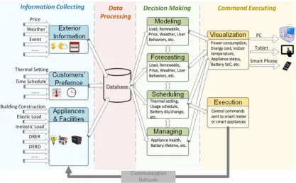
To achieve the above objectives, the proposed HEM operation include four primary
functions: information collecting, data processing, decision making, and command executing, as
shown in Figure 2.1.
15 The information collecting collects three main inputs: ambient information (e.g. outdoor
temperature, solar radiation, and electricity prices), user preferences (e.g. indoor
temperature, task schedule, and cost saving expectation), and measurements from smart
appliances and controllable devices inside the household.
The data processing can process the collected data by specific algorithms, such as data
reorganization and eliminating bad data. Then the data is stored in corresponding
databases.
The decision making consists of four categories of algorithms: modeling, forecasting,
scheduling and managing. The modeling algorithm calculates the model parameters of
load and DER/DESD. The results can then be used by the forecasting algorithm to
produce the energy demand and supply forecast for day-ahead, hour-ahead or intra-hour.
Based on the forecast results, the Scheduling algorithm schedules the appliance usage to
fulfill control objective, such as minimizing the energy cost, enhancing the
comfortableness, and following a load profile target. Management algorithm takes care of
the appliance status and health and gives feedback to scheduling algorithm.
The command executing sends the control commands to the smart switches and
appliances, as well as visualizes the appliance status and energy saving with a Graphical
User Interface (GUI). The two-way communication closes the HEM operation loop,
providing data to the HEM information collecting unit.
2.3
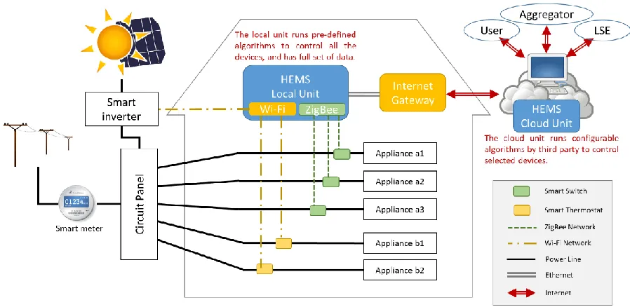
The Proposed Hardware PrototypeThe proposed HEM consists of three main hardware components: an HEM controller, a
16 network. The general topology of proposed HEM is shown in Figure 2.2. This section reviews
the design idea of these three components and their implementation will be discussed in section
2.5.
Figure 2.5 HEM hardware system overview
2.3.1 HEM Controller
The HEM controller is the brain of the system. In order to balance the trade-off between
computational capability and cost effectiveness, the proposed design uses a “hybrid” controller: a
local-centralized unit and a cloud-based unit. The local unit uses control algorithms that requires
less computational resource, while communicates with each of the controllable device/appliance
frequently. It also has the detail energy consumption information in the house. The cloud unit
uses the shared pools of configurable algorithms (developed by a third company) to control
specific large-energy-consume devices (e.g. HVAC and EV) and to cooperate with other HEM to
achieve some upper level control target. The cloud unit can run more advanced control
algorithms with the cloud computer, and it communicates with the household devices less
17 local unit is the main commander for controllable device in the house, but in some cases, the
cloud unit can overwrite or substitute the local unit commands, such as local unit blackout or
power system contingency.
2.3.2 Smart Switch and Smart Thermostat
The HEM uses two types of executors to manage the controllable load: smart switch and
smart thermostat. The smart switch can measure the appliance energy consumption (both voltage
and current), then send this information to HEM controller, and turn it on/off accordingly.
Similarly, the smart thermostat needs to measure the room/water temperature, monitor the house
occupancy, then transmit the data to controller, and decide to turn on/off the device or adjust the
temperature setting.
2.3.3 HEM Communication Network
The HEM operation heavily relies on the communication network in the home area.
There are three types of networking technologies are used in the proposed HEM: Zigbee, Wi-Fi,
and Ethernet.
The Zigbee network is mainly used by the smart switch, which requires low energy
consumption, frequent communication and flexibility of expansion. ZigBee is a short-range,
low-data rate, energy efficient wireless technology based on the IEEE 802.15.4 standard. It uses a
duty-cycle to access to transmit the data, meaning a ZigBee module is active (wakes up) for
18
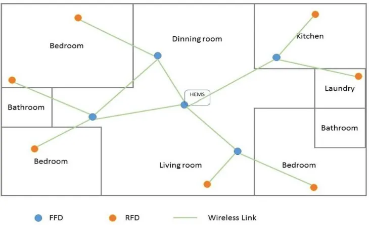
Figure 2.6 Mesh ZigBee network topology of HEM
The ZigBee communication range is between 30 to 70 meters, varied by the obstacle
indoor (e.g. walls). Thus, in my design, it uses the mesh network topology in Figure 2.3. There
are two types of ZigBee devices, full function device (FFD) and reduced function device (RFD).
FFDs can be interconnected with their peers in the mesh topology, while the RFDs can be used at
end nodes. In the smart house, the RFD smart meters or sensors are placed in bedrooms or
bathrooms, FFD smart meters and sensors are placed in hallway or living room. Also there is a
FFD module connecting to the local controller unit as a ZigBee coordinator, working in a beacon
mode to define the duty cycle. The ZigBee module configuration is detailed in the section 2.5.
Other controllable devices, such as smart inverter and smart thermostat, use Wi-Fi
network to communicate with HEM controller. These devices exchange large amount of data
package but in a lower frequency (e.g. every 5 minutes), thus the Wi-Fi network is applied in this
case. The HEM local controller unit collects the data through ZigBee and Wi-Fi, connects to
19
2.4 The Proposed Software Architecture 2.4.1 Software Layers and Interfaces
The proposed HEM software can be divided into three bottom-up layers: library layer,
host layer and application layer, as shown in Figure 2.4.
Figure 2.7 HEM software framework
The bottom layer is the library layer, which is the repository of three main components in
20 HEM setting/parameter: the proposed HEM models different commonly-used household
appliance, such as HVAC, water heater, washer and dryer, etc. Users can input the
appliance setting, such as the thermal setting or usage schedule of the appliances. Also,
the model can allow users to define the price response preference, indicating their
demand elasticity.
External information: this component reads external information that may impact the
HEM operation, including prices, weather information and special events.
Algorithms: the proposed HEM has three main types of algorithms: 1) Forecasting
algorithms provide load or renewable energy forecast for a define horizon; 2) Scheduling
algorithms can schedule load and DRER based on different objectives; 3) Managing
algorithms can be even more extensive, such as battery lifetime evaluation, energy
efficiency monitoring and etc.
The middle layer is called host layer. It has two main components: the database and the
data-flow management. The database stores the historical load profiles and system setting, such
as appliance setting and user preference. The data-flow management controls the time series of
data, and formats the data input and output from/to different layers via the interface.
The upper layer is the application layer. It has a Graphical User Interface (GUI) to
visualize the data and to allow users input the settings. It is also the layer that connects to the
hardware system take in/sent out appliance information.
For research purpose, the HEM software allows researcher to customize some software
components (e.g. control algorithms, pricing schemes, etc.), while the data input/output is
21
2.4.2 HEM Information Flow
There are multiple controllable appliances in a house, but the HEM doesn’t require the
information collected simultaneously in order to avoid more hardware cost. Instead, it measures
the appliances sequentially in a period for multiple times, then averages the measurements of
each appliance as the real-time value. In this design, the smart switch and smart thermostat
measures the appliance 3 times in a minute, and sends the average measurements to HEM
controller as the real-time value. Since the HEM controller has local and cloud units, they have
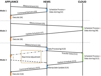
different data process rate. Figure 2.5 shows the information flow among appliance, local
controller and cloud controller. Basically, the smart switch and thermostat measure the appliance
couple times in a minute and send the data to HEM local controller with the average values.
Once the local control gets all the appliance data, it updates the forecast and schedule, and sends
back to those smart devices. The local unit sends some of the appliance data (e.g. HVAC, water
heater) to the cloud unit every 5 minutes. Then based on the cloud unit control command, the
22
Figure 2.8 Information flow among smart device, local and cloud controller
2.4.3 HEM Algorithms Overview
In this thesis, it focuses on developing two main types of algorithm: demand forecasting
algorithm and load scheduling algorithm. There are three key settings for this two algorithms:
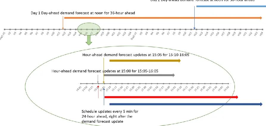
forecast/schedule horizon, update frequency and resolution. Figure 2.6 shows the timeline of
how the forecasting and scheduling algorithm work interactively. In this design, the proposed
HEM forecasts both day-ahead and hour-ahead household electricity demand. The day-ahead
forecast algorithm predicts electricity demand in 15-minute resolution for the next 36 hours. It
updates once a day at 11:45AM, one interval ahead of the forecast horizon (12:00-00:00 next
day). The day-ahead can provide demand forecast for “long-term” schedule, such as charging EV
overnight. For hour-ahead forecast, the forecasting algorithm predicts demand in an hour ahead
with 5-minute resolution, it updates every 5 minutes. The scheduling needs to schedule the load
for 24-hour ahead with a 5-minute resolution. It updates every 5 minutes right after the
23 demand forecast to plan the electricity usage in long-term, such as allocate the dishwashing task,
charging the EV. Meanwhile, with hour-ahead demand forecast, the load scheduling algorithm
can adjust power consumption plan to avoid high demand charge (it is usually based on the
average of power consumption in 15 minutes) or achieve a load profile target. All the forecasting
and scheduling algorithm publish the results one interval before the cover horizon begins.
Figure 2.9 Timeline of forecasting and scheduling algorithm horizon and update frequency
Different than system-level energy management, the HEM needs to use unique
methodologies to forecast and schedule energy demand at household level. In this design, the
forecasting algorithm provides both deterministic and probabilistic demand forecast based on the
granular data from smart devices. It also uses unique methods to evaluate the forecast accuracy.
On the other hand, the scheduling algorithm schedules the controllable device based on their
usage patterns respectively, such as thermostatically-control-appliance, task-base-appliance, and
energy storage device. Moreover, the customer cost saving expectation is considered by
scheduling algorithm, so that it can bridge the gap between user electricity demand elasticity and
24 proposed HEM uses heuristic algorithm, instead of using mathematical optimization algorithm.
In this way, it significantly reduces the computational burden while enhance the algorithm
robustness to the demand uncertainty. The forecasting and scheduling algorithms are presented
in Chapter 3 to Chapter 5.
2.5 HEM Testing System Implementation
In the FREEDM envisioned “Energy Internet” [44], an ac/dc hybrid microgrid system
that enables flexible energy sharing is proposed. A 1-MWh hybrid microgrid testbed called
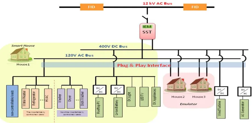
Green Energy Hub [45] is constructed based on several key technologies. As shown in Figure
2.7, the Solid State Transformer (SST) connects the smart house microgrid to distribution grid.
Within the smart house, all household appliances, home-owned energy storage and distributed
generation resources (primarily PV) are managed by an HEM. In this section, it shows the HEM
hardware testbed and the Graphical User Interface (GUI). A showcase demonstrates the HEM
testbed capability.
25
2.5.1 HEM Hardware Testbed
A physical hybrid smart house is setup to provide capability for researchers to validate
control algorithms in a realistic residential microgrid system, as shown in Figure 2.8. The house
includes ac and dc appliances, rooftop PV as DRER, Li-Ion battery as DESD. More specifically,
the dc loads include LED lighting, LED TV, battery (simulating EV) and a dc emulator. AC
loads can be categorized into thermostatically control appliances (TCA) (e.g., HVAC,
refrigerator), task-based appliances (e.g., clothes washer & dryer, EV) and random loads. Hybrid
household loads can also be emulated by ac and dc load emulators (4 kW and 2.5 kW each) so
that the whole smart house test system can be scaled up to 3 houses.
Figure 2.11 Physical HEM testbed in FREEDM System Center
The proposed HEM local controller unit is currently implemented on a PC in the testbed
26 development stage, and it is easier to use GUI to demonstrate the results on PC screen. Actually,
for future deployment, it can be implemented on a mini computer, such a BeagleBone Black or
Raspberry Pi. The local controller unit uses ZigBee network to communicate with smart
switches, and XBee Series 2 is used as the Zigbee RF modules in this design. On the controller
side, it connects with a ZigBee coordinator via RS232. On the smart switch side, the
micro-controller (Microchip PIC16F877A in this design) manages the data flow as shown in Figure 2.9.
Figure 2.12 Smart switch diagram
The proposed HEM cloud controller unit is also implemented on a local PC in order to
communicate with the local unit within university network domain (university network restraints
external visits on internal local machine). To control the smart thermostat, the cloud controller
unit runs a JavaScript program to send JSON file to Ecobee API to change the settings and
events based on the scheduling results.
2.5.2 Graphical User Interface
The GUI provides the users an easy way to set up the simulation and to observe the
step-by-step results. A Matlab-based GUI [30] is developed for the HEM testbed, as shown in Figure
27
① Appliance setting
② Control strategy selection
③ Actual and forecast load profile
④ Renewable energy: PV and energy storage SOC
⑤ Appliance status
⑥ External information
⑦ Appliance monitoring
⑧ Cost comparison before/after control
Figure 2.13 A Matlab-based Graphical User Interface
The HEM GUI is used to modify the resource status and control parameter settings, user
comfort settings, price signals in demand response program, and visualize the results.
1) Appliance parameter setting: For TCAs, whose load profiles are mostly related to outside and
28 For task-based appliances, researchers can set the estimated turn-on time and turn-off time,
during which interval the task should be finished.
2) Control strategy setting: The HEM currently provides three basic control algorithms for
researchers to select: price-cap control, power-cap control and consensus control. For example,
in price-cap control strategy, some appliances will be shut down when the price is higher than
the pre-set price cap. Appliances are turned off according to a priority list calculated by an
optimization algorithm. Power-cap control will shift or shed loads to keep the power
consumption within the pre-set value. The effect on consumer comfort level will be minimized.
Users can also easily implement their control algorithms using the “CUSTOMIZE” function,
which requires users to clarify input/output information in a Matlab programming environment.
3) Input information setting: Before running simulation, input information should be defined,
including pricing scheme, outdoor temperature, and power/price cap.
The main window provides various real-time information, such as actual and forecasted
total power consumptions, solar generation status, battery charging status, and demand response
capabilities. With those displays, researchers can easily access test system status for testing and
validating the effectiveness of their algorithms. In the following section, a demonstration case is
carried out using this GUI to setup and view the results.
2.5.3 A Demonstration Case of HEM Testing System
The showcase demonstrates the capability of HEM scheduling household load under
time-of-use pricing scheme in a typical summer day. The peak hours are from 12 p.m. to 5 p.m
29 charge is not considered in this case. Uncontrolled base load is produced by the load emulators.
The price curve and base-load curve are show in Figure 2.11.
(a) (b)
Figure 2.14 Case setting (a) TOU price curve, (b) base-load
A. Modeling Setup
In each algorithm testing and validation process, the test system needs to be setup in the
following steps.
1) Set up the communication parameters. The users need to configure the smart switching and
metering devices as controllable or metered. In the current test system, the communication
frequency between devices and HEM can be at every 5 second. Although ZigBee technology
allows much faster communication, but communication delay or losses will increase when there
are more devices in the network. This is one of the key reasons that a realistic test system needs
to be used for testing and validating control algorithms.
In addition, a droop control technology is used to regulate the SST output voltage level.
Therefore, there are fluctuations in load measurements. 5-sceond data turns out to be the optimal
communication interval that allows measurements to be collected with good resolution to filter
30 2) Set up the control and monitor parameters for appliances. The following actual appliances can
be used in the test system: air-conditioner (A/C), water heater (WH), clothes washer (CW),
clothes dryer (CD), and dish washer (DW), lighting and TV of both ac and dc, and battery. An
example setting of each controllable appliance is shown in Table 2.1.
3) Select other auxiliary inputs. Auxiliary inputs may be needed based on the control strategies
selected. For example, if one needs to minimize the electric payment under TOU pricing
scheme, TOU prices need to be fed to the communication interface. If peak-shaving is selected,
a signal for executing peak-shaving command will be fed to the communication interface.
Ambient temperatures and user comfort settings and user defined schedules will be needed to
schedule appliance operations.
Table 2.1 Appliances setting
Appliance Rating Setting
A/C 4.5 kW Setpoint: 68 °F, deadband: ±4 °F
WH 2 kW Setpoint: 135°F, deadband: ±15 °F CW 1 kW Scheduled interval: 8 a.m. to 10 p.m. CD 3.5 kW Scheduled interval: 8 a.m. to 10 p.m. DW 1.5 kW Scheduled interval: 10 a.m. to 6 p.m.
Battery 2 kW * 2h --
B. Modeling Results
Figure 2.12 shows the testing results collected from 9 a.m. to 9 p.m., including scheduled
load profile and measured demand curve. We can see that, before peak hour, the demand
increases due to the pre-cooling process and charging battery for later usage. During peak hour,
the battery partly supplies the demand. There is a small peak after peak hours.
It can be seen that the measured demand curve is slightly different from the scheduled
31 processes of appliances can be captured by the metering system, the value of which may mislead
the HEM to trigger a peak shaving signal. This demo case shows the importance of using real
devices to test the HEM algorithms.
Figure 2.13 shows a zoom-in view of the demand curve with corresponding ac and dc bus
voltage at the SST end. Generally, both ac and dc voltage variations are within ±2%, though
voltage spikes can occur when large appliances are switching in and out. This case demonstrates
that providing SST a realistic smart house load can effectively test the SST voltage regulation
algorithms.
32
33
CHAPTER 3 A HOUSEHOLD ELECTRICITY LOAD FORECAST APPROACH FOR HOME ENERGY MANAGEMENT SYSTEM
This chapter introduces the load forecasting algorithms for day-ahead (DA) and
hourly-ahead (HA) residential load forecasting.
3.1 Introduction
Traditionally, load forecasting is often conducted at the system level. This is because the
utility engineers only have access to the load measurements at the feeder head, where
supervisory control and data acquisition (SCADA) data is available. The deployment of smart
meters as well as smart switches possessing metering functions allows the home owners and
utilities to have access to energy consumption data at household level with intra-hour resolution
[70]. To implement different control functions of a Home Energy Management System
(HEMS), a load forecaster is often needed for estimating the energy consumption of appliances
in a scheduling period, which is normally for one day ahead.
Today, many load forecasting techniques have been deployed for forecasting system level
aggregate load, such as linear regression model [71-74], similar day approach [75,76], neural
network model [77-79], support vector machine approach [80, 81], etc. However, at the
household level, because of the randomness in customer consumptions, load is highly volatile.
Therefore, the methods developed for forecasting the aggregated load are not applicable for
forecasting the individual household loads. Some publications have provided study of residential
load forecasting [82, 83]. In [82], it clusters the residential load profiles and summarizes
residential load pattern regarding individual customer attributes, such as house type, number of
residents, age, and number of appliances, etc. [83] uses the smart meter data to identify some
34 household data, so they may not be applicable to forecast individual household demand. Some
researches [83, 84] focus on individual household energy usage disaggregation using either
intrusive or non-intrusive methods, providing information for household appliances modeling.
Some advanced forecast techniques, such as ANN and SVM, are applied on house level load
forecasting [85-87], but they are either system specific or need high computational effect that
HEMS control micro-process can’t handle. Also, most of the residential load forecast related
publications neglect the forecast horizon. Just as system level load forecasting, a household
demand forecaster should consider both short-term (intra hour) and mid-term (day ahead) energy
consumption.
In this chapter, I developed a progressive residential load forecasting method using a
combination of k-mean, multinomial logit regression, and Kalman filter methods to provide the
HEMS with DA and HA load forecast. To obtain the DA load forecast, I used the k-mean based
algorithm to cluster the historical daily electricity load profiles based on their daily weather
conditions. Then, a multinomial logit regression method is applied to subsets of the clustered
load data to forecast the probabilistic of the load level (high, medium, and low) of each 15
minute for day ahead. To obtain the HA forecast, a state-space model with its coefficients
recursively updated by a Kalman filter is used. The forecaster is tested and validated using
realistic smart meter measurements collected from 20 households in Austin, TX. Euclidean
distance and Weighted Mean Absolute Scaled Error (WMASE) are used to quantify the accuracy
of the DA and HA forecast respectively.
The rest of the chapter are organized as following. Section 3.2 presents the forecasting
35 study with 20 household data in both summer and winter case, as well as the household demand
forecast evaluation criteria. Section 3.4 concludes this chapter.
3.2
MethodologyThe proposed forecaster consists of two main processes: DA forecast and HA forecast.
Instead of forecasting a point value, the DA process predicts a 15-minute resolution probability
of three load levels: high, medium, and low, so that HEMS moves schedulable load from higher
demand period to lower demand period. The DA process is updated once a day at noon. The HA
process predicts the deterministic value of load in one hour ahead with 5 minute resolution.
HEMS uses this information to adjust energy usage in real time, for example, if HEMS foresees
a high demand in 10 minutes later, it can postpone a rescheduled dishwasher at that time to a
later time slot. The DA and HA forecaster allows HEMS to largely schedule a load in day ahead
and to fine tune the usage in real time.
The proposed HEM forecasting processes is shown in Figure 3.1. There are two steps in
DA process: (1) find a data set of similar days to the forecasted day based on the weather
condition and day of the week, (2) use the similar days as training dataset to estimate the
parameters in a logistic regression model of load level probabilities. In HA process, it uses the
historical load and weather condition in a state-space model, and applies Karmel filter to
36
Figure 3.17 Household electricity load forecast process: DA and HA
3.2.1 Day-ahead load level probabilistic forecast
Step 1: Clustering load profiles to find similar days
Although residential load profiles vary significantly each day, the probability for high,
medium, and low consumption periods remains stable for similar day types. This is because
weather sensitive loads usually dominate the household energy consumptions. For example,
Figure 3.2 shows the temperature and a realistic household load summer daily change. It
indicates that the load changing interval is correlated with the temperature range during the day.
Thus, we can use the weather information as a criteria to group daily profiles based on an
37
Figure 3.18 A household load and temperature daily change
The inputs of this step include: five months of data (the past two months and three
months last year) and the corresponding weather data (i.e. outdoor temperature, precipitation,
humidity, and wind speed). For example, if March 1, 2018 is the forecasted day, the historical
data set should be January 1st 2018 to February 28th 2018, and February 1st 2017 to April 30th
2018. The output of this step is day groups with similar external conditions. The goal of this
step is to select load profiles that have the highest probability to match the forecast day load
profile.
To cluster the load profiles, the K-mean algorithm is used. Then, the Davies-Bouldin (DB)
index [88] is used to determine the most suitable number of cluster. Eq. 3.1 – 3.5 define the DB
index.
Eq. 3.1 calculates the scatter within the cluster Ci, Xj is the n-dimensional feature vector
assigned to cluster Ci. Ai is the centroid of Ci and Ti is the size of the cluster i.
38 Eq. 3.3 is a measure of how good the clustering scheme is. The lower the value indicates
the better the separation of the clusters and the 'tightness' inside the clusters.
1/ 1 1 i p T p
i j i
j i
S X A
T
(3.1)1
, , ,
1
(
n p)
pi j i j k i k j
p k
M A A a a
(3.2), , i j i j i j S S R M
(3.3)
,
max
i j i i j
D R (3.4)
1 1 N i i DB D N
(3.5)Eq. 3.4 and 3.4 define the DB index, which consider the worst case with the value equals
to Ri,j for the most similar cluster to cluster i. A lower DB index is means that within an
individual cluster, the load profiles are similar to each other and each cluster is well separated.
Once the appropriate number of cluster is identified, the historical day and forecasted day
meteorological data will be used as the input and clustered separately on a 24-hour basis. The
output is the cluster indices of each day, then the days with same index as forecast day will be
used in the second step —probabilistic day-ahead load forecast.
Step 2: Probabilistic forecast with multinomial logistic regression
In the second step, a tri-level load forecast (i.e. high, medium and low) is conducted. This
is because customer consumptions are highly random so capture the exact value of the energy
39 usually important to know when an appliance is turned on whether or not it will create a load
peak. To define the low, medium, and high levels, we used the following criterion:
1. If the consumption is low, then turning on the largest appliance in the household (e.g. a 4
kW air compressor unit) total load can still remain in medium level. Thus, HEMS can
schedule any load to this time slot without creating a peak.
2. If the consumption is medium, then turning on the largest appliance in the household
(e.g. a 4 kW air compressor unit) will make the total load consumption reach 80% of the
predefined peak values.
3. If the consumption is high, then turning on the largest appliance in the household (e.g. a
4 kW air compressor unit) will exceed the predefined peak;
To find the thresholds of the low, medium, and high load levels, a statistical analysis is
conducted based on the predefined peak values and the rated value of the largest appliances. For
example, in Figure 3.3 of a sorted household load in summer time, one can see that the peak
demand is about 11.5 kW. If the largest appliance power rating is 4 kW, we can define the
high/medium threshold is 5.2 kW (11.5*0.8-4), and the medium/low threshold is 1.2kW. With
these threshold, HEMS can schedule the appliance to low load periods, or remove some
40
Figure 3.19 An example of sorted household load
In order to determine the load level probability, a multinomial logistic regression is used
to model the continuous values of predictors (such as temperature, previous load value, time of
the day, etc.) to a probability of load levels between 0 to 1. In a multinomial regression, a logit
function is used to link the odd ratio of an outcome (the probability of an event over the
probability of a reference event) to a linear combination of the predictor variables, so that the
probabilities are restricted between zero and one [89]. Assuming that there are N observations in
the dataset with p predictor variables, and there are J categories of outcome. The problem can be
described as in Eq. 3.6 and 3.7 below.
0 1 1 2 2
1
log ij j j i j i pj ip, 2, , , 1, ,
i
P
x x x j J i N
P
(3.6)
1 1 J ij j P
(3.7)Eq. 3.6 shows that the logarithm of odd ratio for category j to category 1 (reference
category) is a linear combination of predictor variables. The 𝑥𝑖𝑝 represents the p predictor
![Figure 1.1 CAISO's 2013 illustration of the “duck curve”[4]](https://thumb-us.123doks.com/thumbv2/123dok_us/1339032.1166852/15.612.83.530.80.312/figure-caiso-s-illustration-duck-curve.webp)