The Effects of Bus Stops on the Saturation Flow Rate of Signalized Intersections

(1)

HOLT, DANIEL LESTER. The Effects of Bus Stops on the Saturation Flow Rate of Signalized Intersections. (Under the direction of Dr. Joseph E. Hummer)

The total number of vehicle-miles traveled on our roadways has rapidly increased resulting in an increase in traffic congestion and a decrease in the operational integrity of the transportation system. To reduce these numbers of vehicle-miles, agencies attempt to influence and educate users on choosing the alternative mode of travel known as transit. For the potential users to conveniently use transit, agencies must conveniently locate bus stops so as to provide a high level of service. Though transit use has increased to provide

approximately 8 billion passenger trips nationally, the number of vehicles and vehicle-miles traveled on our roadways has not decreased. With these bus stops usually located directly in the traffic stream, detrimental impacts to the traffic flow cannot be avoided as a bus stops and consequently blocks the traffic flow. Therefore, a realistic measure of the effect these transit vehicles have on the transportation system is needed. The 2000 Highway Capacity Manual’s (HCM) Fbb adjustment factor equation found in Chapter 16 uses an average bus blockage time of 14.4 seconds. However, according to Chapter 27 of the 2000 HCM, when an average deceleration and acceleration time of 10 seconds for a bus to enter and exit a bus stop is applied to this 14.4 value, a total bus dwell time of only 4.4 seconds remains to actually serve its passengers. An additional review of Chapter 27 revealed that 15 seconds is a

(2)

on the assumption that the maximum impact of a bus stop occurs during the effective green time period. The near-side bus stop was shown to prohibit the progression of vehicles through the intersection, but that the effective green time and the cycle length were established as non-factors in evaluating this effect. However, the far-side bus stop does allow vehicle progression, but this progression is limited by the available vehicle storage space between the bus and the stop bar and the point in the signal cycle when the stop is performed. These equations were validated using CORISM simulation runs of a simple, saturated roadway network with a single bus route and bus stop that resulted in a simulated and an ideal saturation flow rate. A predicted saturation flow rate was then calculated to compare against the simulated saturation flow rate. Statistical testing and a sensitivity

(3)

(4)

Author’s Biography

The author was born in Sanford, North Carolina, on October 24, 1973, to the parents

of James and Alice Holt. Growing up, the author participated in many social and recreational

activities including the Webelos and Boy Scouts of America, local youth and young adult

baseball, basketball, and soccer leagues and in activities associated with his church. Along

with his parents, the experience of participating in these programs taught the author to set and

achieve lofty goals and high achievements by committing 110% physical and mental effort

towards them and never giving up in pursuit of them.

After relocating to Erwin, North Carolina in the late 1980s, the author graduated from

Triton High School in 1992. Later that year, the author began the pursuit of his Bachelor’s of

Science degree in Civil Engineering at North Carolina State University. During the pursuit

of this degree, the author also spent many hard-earned, but fun-filled, memorable years with

the marching and pep band programs at NCSU as a playing member, as a Drum Major, and

as the graduate assistant. It is these programs that took him to many exciting places

throughout the United States while in support of the Wolfpack of N. C. State including

giving him his first airline trip at the young age of 23.

During the summers between semesters while working toward his bachelor’s degree,

the author gained valuable experience working as an engineering assistant and an engineering

technician with several construction and design units at the North Carolina Department of

Transportation (NCDOT). While working with the band programs at N. C. State and with

(5)

State University with his Bachelor’s of Science degree in Civil Engineering in 1997.

However, the author desired more knowledge to continue his career as a civil engineer.

Later in 1997, with the aide of a graduate assistant and athletic scholarship with the

N. C. State band program, the author began his pursuit of a Masters’ of Science degree in

Civil Engineering at N. C. State. While pursuing and completing his graduate degree, the

author has continued his full-time, professional career as a transportation engineer with the

Traffic Engineering Branch and now as a current member of the Chief Engineer’s Office of

the NCDOT. It was during this time that the author took and passed the Professionals’

Engineering (PE) exam and is now a licensed professional civil engineer with the State of

(6)

Acknowledgements

I wish to thank Dr. Joseph Hummer for his valuable guidance and persistence over the past six years that has helped make this possible. Through the pursuit of my academic and professional career as a transportation engineer, I cannot think of many advisors who have the persistence and belief in a topic to see a professional graduate student through to the end. Not only is this a testament to Dr. Hummer, but it is one to the staff and faculty of the Civil Engineering Department at N. C. State. To these individuals, Dr. John Stone, and Dr. Billy Williams, whose willingness and acceptance to come on at the end is truly appreciative and is something that I may not truly realize, I thank you.

I wish to thank my parents, James and Alice Holt, for their love, support,

encouragement, and, above all, their patience during the past six years. Between the good times and the bad times, your unconditional love, support, and desire for me to achieve a higher education is truly beyond what words could express. For you both I say, ‘I FINALLY did it.’

(7)

I would also like to thank some current and former North Carolina Department of Transportation employees including Jim Rand, Gary Faulkner, and James Dunlop. Your support, understanding, and flexibility during my graduate education and research were greatly appreciated and did not go unnoticed.

Lastly, I would like to express my sincere gratitude to Katherine English. A warm, thoughtless, and patient person who provided unconditional love, support, and

encouragement by giving up countless hours and days so I could finish. Though you only became a part of my life in the past two plus years, it was your inspiration that helped me complete my degree. In hindsight, I think you may have wanted me to have it more than I wanted me to have it. I only hope that life gives me the opportunity to show you my appreciation of your devotion.

Above all, I would be remiss if I did not think God. Things truly happen for a reason. Without him, none of this would be possible.

(8)

Table of Contents

Page

List of Tables ... viii

List of Figures ... x

Chapter 1: Introduction... 1

Purpose and Scope ... 2

Report Outline... 3

Chapter 2: Literature Review... 4

Highway Capacity Manual Treatment ... 4

Curbside Bus Stop ... 7

Reserved Bus Lanes/Bus Bays... 9

Queue Jumpers... 10

Traffic Signal Bus Preemption... 11

Transit Priority Traffic Signal Timing... 12

Contra-Flow Bus Lanes ... 14

Chapter 3: Alternative Selection... 17

Selection Summary ... 22

Chapter 4: Equation Formulation... 23

Near-Side Bus Stop... 23

Far-Side Bus Stop ... 25

Chapter 5: Simulation Approach and Results... 31

Method of Analysis... 31

Far-Side Bus Stop ... 34

Far-Side Simulation Results ... 37

Far-Side Statistical Testing ... 45

Comparison against the HCM Method for the Far-Side Bus Stop ... 53

Far-Side Equation: Sensitivity Analysis ... 54

Near-Side Bus Stop Experiment ... 58

(9)

Comparions against the HCM Method for the Near-Side Bus Stop... 64

Chapter 6: Conclusions and Recommendations ... 66

Future Work... 68

List of References ... 70

Appendix A... 71

(10)

List of Tables

Page

Table 1: Bus Blockage Adjustment Factor Values, 1994 HCM... 6

Table 2: Alternative Evaluatin Matrix ... 18

Table 3: CORSIM Case Inputs – Far-Side Bus Cases... 36

Table 4: Average Simulated and Predicted Flow Rates – Far-Side Bus Cases ... 39

Table 5: T-test Results of Dwell Time, 15 sec vs 30 sec... 45

Table 6: T-test Results of Effective Green Time, 40 sec vs 60 sec ... 45

Table 12: T-test Results of the Proportion of Right-Turns, 0.00 vs 0.25 ... 48

Table 15: T-test Results of Bus Stop Location, 100 feet vs 250 feet... 50

Table 16: T-test Results of Predicted vs Simulated Flow Rates for Accepted Cases... 51

Table 17: T-test Results of Cases D, E, and F ... 52

Table 18: T-test Results of Cases G, H, I, and L ... 53

Table 19: T-test of Simulated Flow Rates vs HCM Flow Rates for Far-Side Stops ... 53

Table 20: T-test of Predicted Flow Rates vs HCM Flow Rates for Far-Side Stops ... 54

Table 21: Case Inputs for Sensitivity Analysis... 56

Table 22: Inputs for Near-Side Cases ... 59

Table 23: Average of Simulated and Predicted Saturation Flow Rate Values - Near-Side Cases ... 60

Table 24: T-test of Predicted Flow Rates vs Simulated Flow Rates for Near-Side Stops.... 62

(11)

Table 28: T-test of Simulated Flow Rates vs HCM Flow Rates for Near-Side Stops... 64

Table 29: T-test of Predicted Flow Rates vs HCM Flow Rates for Near-Side Stops... 64

Table A1: Far-Side CORSIM Results, Cases 1 - 12... 72

Table A2: CORSIM Results and Calculations, Case 14... 73

Table B1: Near-Side CORSIM Results, Repetitions 1 - 5... 82

(12)

List of Figures

Page

Figure 1: Diagram of Time Period One (P1)... 27

Figure 2: Diagram of Time Period Two (P2) ... 28

Figure 3: Diagram of All Three Time Periods... 29

Figure 4: Simulated CORSIM Network ... 32

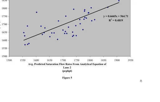
Figure 5: Avg. Predicted Saturation Flow Rates vs Avg. Simulated Saturation Flow Rates (Accepted Cases Only) ... 42

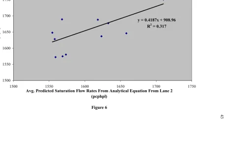
Figure 6: Avg. Predicted Saturation Flow Rates vs Avg. Simulated Saturation Flow Rates Only for Cases with Suffixes D, E, F... 43

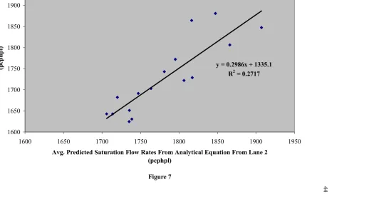
Figure 7: Avg. Predicted Saturation Flow Rates vs Avg. Simulated Saturation Flow Rates Only for Cases with Suffixes G, H, I, L... 44

(13)

Chapter 1: Introduction

In the past fifty years, the total number of vehicle-miles traveled on America’s

roadways has rapidly increased resulting in an increase in traffic congestion and a decrease in

the operational integrity of the transportation system. In an attempt to reduce the number of

vehicles and miles traveled, agencies attempt to influence and educate transportation users to

choose alternative modes of travel. Their goal is to advocate public transportation and

person-trips rather than vehicular trips to reduce the number of vehicle-miles, thereby

decreasing the amount of traffic congestion. (1)

On a typical weekday, the transportation system may experience more than seven

million workday commuters using public transportation with some additional thirty million

persons depending on it to reach other destinations. Transit stops may accommodate an

estimated eight billion passenger trips nationally. (2)

For these eight billion public transportation passengers, it is necessary for agencies to

locate and design bus stop locations that provide good service, while trying to minimize any

effects to traffic. Besides stopping traffic to serve passengers, transit vehicles are larger,

slower, and less maneuverable than average automobiles and cause detrimental impacts to

the traffic flow and the facility. The effects of these transit vehicles in the traffic flow can be

observed as a reduction in corridor speed or as an increase in vehicular queues and delay. (1)

Ultimately, better measures of the effects these transit vehicles and their stops have on the

(14)

Purpose and Scope

As it currently stands, the NCDOT does not have a formal policy concerning the

construction design or placement of bus stops with respect to its location from intersections

on state maintained roadways in the State of North Carolina. However, a joint effort between

the City of Charlotte and the North Carolina Department of Transportation is currently

underway to develop such a policy for state maintained roadways located within the authority

of the City of Charlotte. As this joint effort continues, it is an objective of this research to

provide recommendations for these agencies to consider in their development of a formal

policy by indicating the potential effects to the transportation system of locating a bus stop

near a signalized intersection.

As a result, the goal of the research is to analyze the effects of a bus stop on the

saturation flow rate of a signalized intersection through the development of analytical

equations with simple, available inputs that estimate those bus stop effects. The equations

will be validated using a simulation of a simple, saturated roadway network with a single bus

route and a single bus stop. As the literature review in Chapter 2 will show, previous

research that investigated the implementation of alternative bus stop designs and treatment

did not evaluate their effect to vehicular traffic during a saturated flow condition. In

addition, keeping the simulation experiment simple allows the researcher to reduce the

number and complexity of the simulation runs as well as minimize the number of factors in

the experiment thereby creating credible and usable results. The validated equations

(15)

saturation flow rate. This, in turn, will allow traffic engineers to quantify the effects of bus

stops on the highway system using standardized procedures.

Report Outline

The process of evaluating the effect bus stops have on the saturation flow rate began

with a literature review. This review involved the use of Internet databases, physical searches

of personal, academic, professional, and other resource libraries, and communication with

contacts in the transportation industry. After completion of this review, criteria were

compiled to evaluate the types of bus stops contained in the literature review for evaluation

in this research.

An evaluation matrix examined each alternative bus stop design based on the

availability of analysis tools to evaluate the design, their effects on traffic capacity, the safety

of the bus stop, and their use in North Carolina. After selecting the alternatives for analysis,

analytical equations were developed to predict the effect of these bus stop alternatives on

saturation flow at signalized intersections. A section of this document describes how the

equations were developed and how the assumptions were made. Next, experimental runs

were created using the CORSIM program to validate the performance of the equations. After

completion of the CORSIM runs and after performing the appropriate statistical tests to

assess the validity of the analytical equations, recommendations were made for a future

(16)

Chapter 2: Literature Review

The intent of the literature review was to identify any research that has been

performed regarding the effects of a bus stop as it relates to the operational performance of a

signalized intersection. Once this research was identified, questions surrounding the validity

of the results were compiled. These questions led to the creation of criteria used in

evaluating this past research to formulate the scope, design, and limitations of the research.

Highway Capacity Manual Treatment

Prior to the year 1965, approximately 1,600 intersection studies were completed for

the Highway Capacity Manual (HCM) for use in level of service and capacity evaluations in

the HCM. As a result of these studies, it was found that the proportion of heavy vehicles was

a factor that influences an intersection’s operational performance. It was concluded that the

degree of this impact was dependent on the type of vehicle, its weight-power ratio, and its

size and turning characteristics. It was also concluded that the effect of a bus and its stop on

an intersection depended on the area of the city in which it was located (central business

district, CBD, or suburban stop), the street geometrics and channelization, any on-street

parking conditions, and the number of buses. (3) Much of this analysis structure survives in

the current (2000) version of the HCM.

Under prevailing traffic conditions, the capacity of a signalized intersection is

calculated and measured in terms of a saturation flow rate – the equivalent hourly rate at

(17)

indication is available at all times and no lost times are experienced. This saturation flow is

measured in terms of passenger cars per hour per lane (pcphpl). (4)

The calculation begins with the selection of an ideal saturation flow rate, So, currently

estimated as 1,900 passenger cars per hour per lane (pcphpl). This ideal flow rate, So, is then

adjusted for field conditions through the utilization of adjustment factors, F, as shown in the

following equation: (4)

S=SoFwFhvFgFpFbbFaFluFltFrtFlpbFrpb , (Equation 16-4, 2000 HCM)

where,

S = saturation flow rate for subject lane group; Fw = adjustment factor for lane width;

Fhv = adjustment factor for heavy vehicles in traffic stream; Fg = adjustment factor for approach grade;

Fp = adjustment factor for existence of a parking lane or parking activity; Fbb = adjustment factor for blocking effect of local buses;

Fa = adjustment factor for area type; Flu = adjustment factor for lane utilization;

Flt = adjustment factor for left turns in lane group; Frt = adjustment factor for right turns in lane group; Flpb = pedestrian adjustment for left-turn movements; and Frpb = pedestrian-bicycle adjustment for right-turn movements.

Of these adjustment factors, Fbb, the bus blockage factor, accounts for the effect of a bus stop

that is located within 250 feet, either upstream or downstream, of the signalized intersection.

The adjustment value is based on the number of lanes in a lane group and the number of bus

(18)

the HCM with negligible numerical changes between the values that can be attributed to

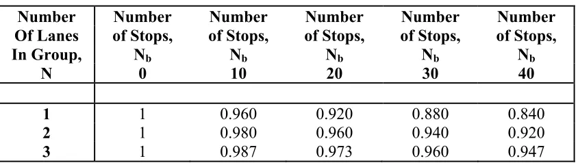
mathematical rounding. Table 1 shows the table for finding Fbb from the 1994 HCM.

Table 1: Bus Blockage Adjustment Factor Values, 1994 HCM

Number Number Number Number Number Number Of Lanes of Stops, of Stops, of Stops, of Stops, of Stops,

In Group, Nb Nb Nb Nb Nb

N 0 10 20 30 40

1 1 0.960 0.920 0.880 0.840

2 1 0.980 0.960 0.940 0.920

3 1 0.987 0.973 0.960 0.947

However, beginning with the 1994 HCM, an equation to directly calculate the value

of the bus blockage factor was introduced: (4)

Fbb = (N – ((14.4Nb)/3600)) / N (Exhibit 16-7, 2000 HCM)

In this equation, ‘N’ represents the number of lanes in the lane group and ‘Nb’ represents the

number of buses stopping per hour. This equation was also recommended for use when the

number of bus stops per hour exceeded 40 in an hour. The 2000 HCM omits the table of bus

blockage adjustment values and only a calculation utilizing the equation is now available.

In the 2000 HCM equation for bus blockage, the value of 14.4 (seconds) represents

the average bus blockage time per bus stop. Of the available bus characteristics that can

impact a facility’s traffic flow, the blockage time is perhaps the most critical. Simply

defined, the blockage time is the amount of time a bus blocks a travel lane. The capacity

reduction to the intersection is directly correlated to the amount of blockage time. A portion

(19)

time. Though a field calculation of dwell time is possible, in the absence of field data,

Chapter 27 of the 2000 HCM recommends commonly-accepted values of dwell times from

15 to 60 seconds. The remainder of the blockage time is what is necessary for the bus to

decelerate to a stop and to accelerate from a stop. Chapter 27 of the HCM recommends

typical values of five seconds for deceleration and five seconds for acceleration for a total of

ten additional seconds. (4) When this additional ten seconds is applied to the 14.4 value in

Chapter 16, it is unrealistic to assert that approximately 4.4 seconds is available to serve the

passengers at a bus stop.

A review of the differing bus blockage and dwell times from Chapters 16 and 27

reveal an additional discrepancy in the Fbb adjustment factors from Table 1. If an

HCM-recommended dwell time of fifteen seconds is coupled with the additional ten seconds from

the bus maneuvers to equate a total bus blockage time of twenty-five seconds and as the

number of bus stops (Nb) increase from zero to one per minute, with all other factors held

constant and ideal, the total Fbb adjustment factor increases from zero to forty-two percent.

However, using a bus blockage time of only 14.4 seconds per stop, the HCM adjustment

factor approaches, at most, a twenty-four percent adjustment as the value of Nb approaches

one per minute. Therefore, this research will question whether the value of 14.4 is

appropriate.

Curbside Bus Stop

A common design of most bus stops is the curbside bus stop. With these types of

stops, the bus performs its stop in the actual travel lane. Typically, this stop is either located

(20)

the stop bar (i.e., the far-side stop). Located either upstream or downstream, it is the

stopping of the bus in the travel lane that is the curbside’s bus stop greatest impact to the

traffic flow. To analyze the impact to traffic operations, a portion of Transit Cooperative

Research Program (TCRP) Project A-10 was set aside to study how bus stops influenced both

roadway and pedestrian traffic for both the curbside and bus bay types of bus stops on

suburban arterials. (5) The TCRP project visited and collected data at fourteen sites located

in Arizona, Michigan, and California. These field studies indicated that through vehicles

with the far-side bus stop encountered more delay than those with a near-side bus stop. The

project noted that buses stopping at near-side stops, particularly at signalized intersections,

overlapped with the red phases of the traffic signal which resulted in less delay.

During the computer simulation portion of the study, researchers concentrated their

investigations on using such factors as vehicle speeds and maximum queue lengths behind a

stopped bus. The researchers calibrated the models by comparing field studies for travel time

and queue lengths with the data generated by the computer model. In the outputs, a

relationship between vehicle speed differences and bus dwell times was discovered for dwell

times of twenty, forty, and sixty seconds. In its conclusions, the study reported that the bus

bay stop, where an exclusive lane or turnout is provided to remove a bus from the traffic

stream to perform its stop, showed advantages over curbside stops in increased average

vehicle speeds at simulated traffic volumes of 250 and 350 vehicles per hour (vph). (5)

The results of this research indicated, as expected, that when a bus stop is out of the main

travel lane the impact to traffic operations is minimized. However, factors related to such

(21)

roadway geometry were not identified as being significant in their field studies or in their

computer modeling. In addition, though a plot of the speed difference versus the total traffic

volume was presented, the impact to the saturation flow was unknown.

Reserved Bus Lanes/Bus Bays

A bus bay is a designated area adjacent to a roadway that allows for the loading and

unloading of passengers while removing the transit vehicle from the adjacent traffic flow.

The removal of buses from the traffic flow allows the facility to maintain a consistent traffic

flow without significant interruption (5). Transportation analysts with the IBI Group in

Toronto, Ontario, Canada, researched the impacts of bus bays on a surface street corridor in

Toronto. The research team wanted to conduct a corridor study to evaluate whether bus bays

are successful in improving bus and corridor performance. Rather than physically

implementing bus bays into an existing transportation system, they chose simulation with the

TRANSYT-7F program, a macroscopic simulation and signal-optimization program, to

model traffic conditions. The decision to use TRANSYT-7F resulted from its history of

analyzing transit priority measures and its estimates of delay based on the principles

associated with the theory of deterministic queuing.

The experiments employed basic study cases that evaluated the ‘before/after’

conditions of transit and traffic flow operations during AM and PM peak hour of traffic

volume. The ‘before’ case consisted of the shared-lane scenario (where a bus and

automobile utilize the same lane) with a curbside bus stop. The ‘after’ case simulated the

existence of a bus bay that separated the transit vehicle from the adjacent traffic flow. To

(22)

conducted to collect data on traffic signal delay, total vehicular travel time, and bus stop

dwell time. Using field validation, the local saturation flow rate was calculated.

The research results showed that the average delay and travel time for the adjacent

traffic increased by 28% and 15%, respectively, with a 15% decrease in average speed, as the

bus dwell time increased to serve the increased bus ridership. Likewise, buses experienced a

14% reduction in average delay and a 9% reduction in average travel time with an 11%

improvement in average speed. As can be seen by these results, the improvements in bus

operation were exceeded by the degradation impacts to the adjacent traffic stream. However,

it was unclear whether the increased bus ridership and dwell time was attributed to a possible

traffic shift to other surface street routes with the implementation of bus bays or whether

users actually switched to the transit mode. (6)

As the research noted, the use of the TRANSYT-7F program resulted in unreliable

capacity estimates as the degree of saturation approached 100%. However, it is at the

saturated condition where the greatest detrimental impact of a bus stop on an intersection’s

capacity should be measured. Therefore, for this research, a computer simulation program

will be selected that will allow saturated traffic conditions to be analyzed so that the

detrimental impact to an intersection’s capacity can be quantified.

Queue Jumpers

A portion of TCRP Project A-10 also studied the queue jumper, a unique type of bus

bay, in a transit-priority design that provides the bus the ability to bypass queued vehicles at

a signalized intersection to reach a far-side bus stop. This bypass maneuver is accomplished

(23)

intersection. This exclusive lane allows for a direct movement to a far-side bus stop. A

queue jumper removes a bus from the traffic flow and allows it to make its stop while being

removed from the traffic flow. A queue jumper study was performed to develop possible

recommendations for queue jumper designs at far-side bus stops. The potential benefits of a

queue jumper for buses are measured in terms of travel time savings and an increase in

speed. To estimate the advantages of a queue jumper, the travel time savings were converted

to speeds. The research indicated that the bus benefits of a queue jumper were noticed once

traffic volumes exceeded 250 vph. (5) A queue jumper is an example of a transit-priority

design that improves the efficiency and operation of the transit vehicle. By removing a

transit vehicle from the main traffic flow via an exclusive lane, its impact to saturation flow

rate has already been minimized. Therefore, this bus stop design would not be a good

treatment to analyze for its effect on the saturation flow rate.

Traffic Signal Bus Preemption

Khasnabis, Karnati, and Rudraraju discuss traffic signal preemption techniques that

provide preferential treatment for bus progression through signalized intersections. (7) This

priority is achieved via green extension, red truncation, or red interruption. Green extension

increases the green time by a specified amount. Red truncation terminates a red phase with

the injection of a short green phase that is not a part of the normally-programmed green

phase. The lack of contiguity with using a red truncation calls for additional time to be

incorporated into the clearance phase. With each technique, an increase in green time, a

reduction in delay, a reduction in queue lengths, and an increase in vehicle capacity are the

(24)

To analyze this signal preemption, the researchers chose the NETSIM software. The

primary objective of the research was to develop a procedure for assessing the operational

impacts of implementing the signal preemption. To perform the research, a series of

signalized intersections on a primary bus route in Ann Arbor, Michigan was selected for data

collection and validation. To minimize the complexity of the data collection, a number of

signalized intersections were excluded based on their complex phasing and actuated signal

operations.

At the outset, it was suggested that bus preemption may adversely impact side street

traffic operations as the preferential allocation of effective green time for the main street

increases vehicular delay and queue length on remaining approaches not given preferential

treatment. However, the paper indicated that no preemption technique was validated in its

entirety with this research nor should it be used to evaluate the results of bus preemption on

intersections, and that further research is necessary to estimate a net savings in vehicular

delay. (7)

Transit Priority Traffic Signal Timing

The Southwest Region University Transportation Center presented research into

modifying the existing transportation infrastructure in lieu of the higher cost of physically

reconstructing a transportation infrastructure. (8) To offset an increased traffic demand and

congestion, the encouragement of high occupancy vehicles (HOV) such as surface street

buses, as an alternative in meeting travel demand, was introduced. This research noted that

one method of promoting the use of mass transit by increasing its operational efficiency in

(25)

research team believed that the signal timing adjustments should be re-focused on the entire

transportation system and not just at a single point, i.e. the transit vehicle.

To model and simulate the impacts of implementing any signal timing priority

scheme, the TRAF-NETSIM software, a microscopic simulation program that analyzes

individual vehicles as they interact with other vehicles, was chosen. The simulation used

signal timing methods such as green extension or red truncation over a run time of sixty

minutes to evaluate any effect from a signal adjustment. The researchers simulated traffic

volumes that ranged, in increments of 10%, from 0% to 100% of saturated flow. In each

simulation run, a transit priority cycle was inserted in lieu of the normal signal timing plan

once every ten minutes to simulate a ten-minute bus headway. After completing these

NETSIM runs, an increase in travel delay was observed along with a degree of uncertainty as

to whether the bus benefits of the transit priority signal timing scheme outweighed the delay

increase incurred by the remaining vehicles.

The NETSIM outputs indicated that once the level of saturation reached 100%,

priority signal timing schemes yield no significant advantage. The results further noted

limited success utilizing the green extension treatment method with a near-side bus stop.

However, the research indicated that priority methods might have success with far-side bus

stops since the measure of effectiveness is no longer a direct function of the bus dwell time.

The researchers further noted that the use of the green extension method could allow traffic

to operate under its normal signal timing scheme. The results showed a positive effect in that

transit vehicles gain a significant share of trips through the use of a priority signal timing

(26)

cycle length, transit delay, and vehicular delay can in fact decrease. However, it should be

noted that the runs involved with this research concentrated on off-peak times of operation.

Therefore, the researchers indicated that an emphasis on peak hour operations when traffic

corridors are operating at their highest possible degree of saturation needs to be performed.

(8)

Contra-Flow Bus Lanes

In order to improve surface street traffic operations, Rouphail presented research

involving the use of contra-flow bus lanes and the programming of traffic signal settings to

minimize passenger delays rather than using the conventional signal timing method of

minimizing vehicular delays. (9) The research intent was to evaluate the relationship between

bus performance and signal priority techniques. A contra-flow bus lane provides a bus an

exclusive lane to travel and perform its operation in the opposite direction of the adjacent

traffic flow. The advantage of a contra-flow bus lane is that any bus blockage of traffic flow

is eliminated and the adjacent traffic flow is not impeded, although cars lose the use of one

lane.

The research reflected actual field observations on a typical Chicago, Illinois,

downtown street where a contra-flow bus lane was installed in 1980. The conclusions

indicated that bus operation dramatically improved with the dedication of an exclusive lane

to bus traffic. This improvement was observed by an increase in the overall bus speed on the

route. This separation of bus traffic from the normal traffic flow was viewed as a means of

(27)

To evaluate the effectiveness of the contra-flow bus lanes and a traffic signal timing

priority schemed designed to minimize passenger delays, the researchers chose the

TRANSYT-7F program. In using this program, six scenarios were developed for analysis.

However, with the density of the pedestrian traffic in the study area, the default saturation

flow rate in TRANSYT-7F was revised.

The TRANSYT-7F model results showed that the degree of operational improvement

was dependent on whether the buses operated in mixed traffic conditions or in exclusive

contra-flow lanes. In addition, the research noted that the total number of vehicle-miles for

the nonbus traffic did decrease after the implementation of the contra-flow bus lane. The

research noted that some of the improvements in nonbus traffic could be attributed to the

increased bus ridership. Though a ridership increase and a lower total of vehicle-miles

traveled with the implementation of the contra-flow bus lane has a positive impact on a

congested arterial, the impact of these bus treatment measures on the saturation flow rate was

still not known. (9)

The literature review uncovered several research projects that looked at different

strategies and bus stop treatments at intersections to improve bus performance while also

attempting to reduce the magnitude of traffic congestion on our nation’s roadways. The

analysis for each of these strategies typically resulted in an improvement and enhancement of

the bus ridership and operations. However, as buses and vehicles predominately share the

same travel lanes, the magnitude of the bus operation improvement was usually at a cost to

the vehicular portion of the traffic stream. Whether it was an increase in bus ridership that

(28)

signal network was optimized for bus vehicles to improve or maintain its service, it is the

vehicular traffic that is negatively impacted. This impact to vehicular operations was not

accurately estimated or, at times, even noted in the research analysis. Though certain

research reported the degradation to adjacent vehicles in terms of speed or delay, a more

basic measure of the impact a bus stop has on an intersection, its saturation flow rate was not

quantified. Though computer software such as TRANSYT-7F was used to evaluate traffic

operations, at the time the computer software included flaws in its modeling that can

inaccurately report the level of operations, especially at saturated conditions. In addition,

most of the research and computer software had its handling of bus operations and its effects

on the traffic stream rooted in the Highway Capacity Manual. In using the manual, it is

observed that the handling and characteristics of buses and bus stops from the average or

typical bus blockage time to the equations to use differ even between the chapters of the

same manual.

With the clear discrepancies in the average bus blockage times found in Chapters 16

and 27 of the Highway Capacity Manual, 14.4 and 25 seconds respectively, and the lack of

any conclusive analysis in the literature review of the impacts that an alternative bus stop

design and treatment have on an intersection’s saturation flow rate, this research will focus

its efforts on developing analytical equations that serve to more accurately estimate and

quantify the bus blockage adjustment factor for use in the calculation of an intersection’s

(29)

Chapter 3: Alternative Selection

Upon completion of the literature review, a list of bus treatments that have the

potential for further analysis was compiled. This list was narrowed in an evaluation matrix

that uses criteria that arose during the literature review that measure the scope of the impacts.

The first criterion measures the potential use and application of the bus stop on roadways in

the State of North Carolina. The second criterion measures the ability of computer software

such as CORSIM, TRANSYT, Synchro, and HCM to analyze an intersection containing a

bus stop. The next criterion measures the effects the bus stop treatment has on the vehicular

safety of the adjacent traffic volume. This criterion measures the expectation of a transit

vehicle performing a stop and how this expectation alters driver behavior. The remaining

criteria measure the use of a particular type of bus stop and its effect on the capacity of a

signalized intersection and the effect it can produce on transit operations in terms of whether

transit can deliver a high quality of service to its users. Each bus stop treatment was assigned

a categorical score - positive, negative, or neutral benefit – based on its comparison to a

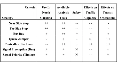
signalized intersection without a bus stop. Presented in Table 2 is an evaluation matrix that

shows the score for each bus stop treatment in each criteria category that was used in

(30)

Table 2: Alternative Evaluation Matrix

Criteria Use In Available Effects on Effects on

North Analysis Safety Traffic Transit

Strategy Carolina Tools Capacity Operations

Near Side Stop ++ ++ - - - - -

Far Side Stop ++ ++ - - - - -

Bus Bay + ++ + + +

Queue Jumper - + - N + +

Contraflow Bus Lane - - ++ + ++ + +

Signal Preemption (Bus) + + N - - +

Signal Priority (Timing) + + N - - +

Legend

+ + = very positive effect + = somewhat positive effect N = neutral effect

- = somewhat negative effect - - = very negative effect

Alternatives that create only marginal results as well as those that would create a

complex experimental design beyond the constraints of the research were not selected. After

considering the results of the literature review and the evaluation matrix, two alternatives

emerged as promising for further analysis. In the following sections, the two alternatives

selected for further analysis are discussed with the remaining sections examining those

alternatives that were not selected.

Curbside bus stops, both near-side and far-side, appropriately satisfied the

(31)

selected as the most promising alternatives for further analysis. These common types of bus

stops are perhaps the easiest and most convenient for passengers and transit vehicles to use.

However, these curbside stops are perhaps the most detrimental to the traffic flow.

As a curbside stop occurs in the traffic flow lane, they impede traffic progression and

reduce the number of vehicles that an intersection can process. With the relative ease and

ability to model these types of stops, obtaining credible results and conclusions can be

accomplished within the constraints of the research.

Though not a common bus design treatment on North Carolina’s roadways due to the

right-of-way necessary for it, a bus bay bus stop is a condition where a transit vehicle uses

an exclusive travel lane or turnout to perform its stop. A major advantage of the bus bay is

the opportunity it provides for a bus to perform a stop while removed from the traffic flow.

This opportunity assists in minimizing the impact the stop has on the adjacent traffic flow.

With the stop performed outside of the traffic flow, the surrounding vehicles can continue

their normal traffic progression.

Though the bus bay allows a stop to occur outside the traffic flow, a degree of

concern is introduced when the transit vehicle exits and re-enters the traffic stream. Due to

the nature of the transit vehicle, the amount of time and space necessary for it to decelerate

and accelerate before and after the stop may alter the behavior of the adjacent traffic flow.

However, with an overall positive benefit to the traffic flow of a bus bay, it was not selected

for further analysis.

An uncommon design in North Carolina, a queue jumper is a type of bus stop that is

(32)

turn lane, allows a bus to bypass a standing queue, if it exists, and to progress through the

intersection to perform a stop in an extension of this exclusive lane on the far-side of the

intersection. Though the frequency of implementing this type of stop is low, it does provide

benefits to transit similar to a bus bay. By utilizing an exclusive lane to bypass a vehicle

queue, a bus can avoid delay in performing its stop. In addition, the exclusive transit lane

allows the normal traffic progression to continue without impedance from a stopped bus. As

is the case with a bus bay stop, the deceleration and acceleration associated with the bus

exiting and re-entering the traffic stream can provide some impacts to traffic operations.

Though the initial exiting and re-entering of the bus into the traffic stream will degrade

traffic operations, the traffic progression is not forced to endure additional effects that result

from a stopped bus. With an overall positive impact to the adjacent traffic flow, a queue

jumper was not selected for further analysis.

Extremely uncommon in North Carolina, a contra-flow bus lane is an exclusive

transit lane that allows transit vehicles to perform their stops while traveling in the opposite

direction of the vehicular traffic flow on a one-way street. The potential for this design to

provide a positive benefit to transit operations and the surrounding traffic flow may be

substantial where it can be implemented. As a bus performs its functions outside of the

traffic flow, the acceleration and deceleration characteristics and the dwell time that

accompanies each stop is not a direct impact to the adjacent traffic flow. However, a degree

of concern exists where these contra-flow lanes intersect and interact with the normal traffic

flow. Also, a contra-flow lane does reduce the number of lanes available for cars, and there

(33)

analyzed in a computer simulation program, with its significant potential of providing

positive benefits to the surrounding traffic operations, its effect on the saturation flow rate

will be minimal. Therefore, a contra-flow bus lane was not selected for further analysis.

Where implementing physical treatments for a bus and a bus stop are not feasible, the

use of traffic signal preemption is a possibility. The objective of this or any other type of

preemption technique is to provide some kind of preferential treatment to ease the movement

of a particular vehicle or approach. This preferential treatment is usually achieved at the

expense of the other users of the network. Various preemption techniques may involve

extending the green time for an approach or by truncating a phase to induce a red signal

indication to allow for a preferential movement. However, the measures of the benefits or

costs to an intersection’s capacity and traffic progression are difficult to quantify. These

preemption techniques are difficult to analyze in a computer simulation program as a

complex experiment design is needed. For these reasons, this technique was not selected for

further analysis.

The last alternative studied in the literature review was transit priority in traffic

signal timing. As noted by Rouphail (4), the standard in developing a traffic signal timing

plan is to use the minimal amount of green time necessary to process the maximum amount

of vehicles possible while vehicular delay is minimized to the maximum extent possible. If

this standard is followed, in theory, the capacity of the intersection and its traffic progression

are optimized. However, when a signal timing plan is developed with its focus to ensure that

(34)

published stop schedule, the magnitude and severity of the impacts to the surrounding traffic

flow and approaches are secondary considerations.

Selection Summary

Based on the criteria that were compiled after the literature review, two alternatives,

the near-side and far-side bus stops, were selected for further analysis and experimentation

with a computer simulation program. These alternatives have the potential to produce a

significant impact to an intersection’s saturation flow rate. As for the remaining alternatives

that were not selected, they either already have a positive benefit to the surrounding traffic

flow (bus bay, queue jumper, contra-flow lane) or they focus on improving bus operations

and not necessarily improving the adjacent traffic flow (signal preemption, signal timing) and

(35)

Chapter 4: Equation Formulation

The Highway Capacity Manual (4) is the pre-eminent traffic operations analysis

reference in use in the United States. In reviewing the HCM, we see that the bus blockage

time includes the time to serve the passengers, or dwell time, and the deceleration and

acceleration time involved in entering and exiting the bus stop. According to Chapter 27 of

the HCM, a typical dwell time value, Dw, for an outlying (suburban) stop is approximately

fifteen seconds with an accepted value of five seconds for the deceleration and five seconds

for the acceleration time (ten seconds total) for the bus at the bus stop. Given a typical

outlying stop, the typical bus blockage time would be twenty-five seconds (Dw +

deceleration + acceleration, or 15 + 5 + 5). This pause in vehicle movement has its

maximum impact on the saturation flow rate when it occurs during the effective green time

period of the traffic signal cycle.

Near-Side Bus Stop

When a near-side bus stop is assumed with random bus arrivals, the chance that a bus

stop occurs during the effective green time (g) is equal to the g/C ratio, or the effective green

time to total cycle length time (C) ratio. With the g/C ratio applied to the value of the total

bus blockage time (BT) for all buses that stop (Nb) in a given time frame (e.g., one-hour), the

proportion of the green time blocked for that one-hour time period is expressed in the

(36)

Proportion Blocked = Nb * BT * g/C

For example, if a cycle length of 100 seconds has an effective green time of 40 seconds and a

bus blockage time of 25 seconds with 6 bus stops occurring, the following proportion of one

hour of green that is blocked by the bus given these arbitrary values is as follows:

Nb * BT * g/C = 6 bus/hour * 25 sec/bus * (40/100) sec/sec

= 60 sec blocked/hour

Given the units that remain and that the equation is for the proportion of one hour of green

that is blocked, to find the proportion of a real hour that is blocked, we need to divide by the

g/C ratio times 3,600 seconds, or 1,440 seconds, as follows:

Proportion of hour blocked = 6 bus/hr * 25 sec/bus * (40/100) sec/sec = 60 sec blocked (40/100) sec/sec * 3600 sec/hr = 1440 sec of green time

The result of this example is that 0.04167, or 4.167%, of the hour is blocked by the bus. It is

clearly observed that the g/C ratio factors out and is of no consequence in evaluating the

effect of a near-side bus stop on the saturation flow rate. In the equation for the bus blockage

adjustment factor, Fbb in the HCM, the value of 14.4 represents an average bus blockage

time, in seconds. Noting Chapter 27 of the HCM and the recommended value of the

blockage time for a typical bus stop of 25 seconds, the value of 14.4 can be questioned.

Accounting for the fact that a lane group may contain more than one lane, the saturation flow

rate adjustment factor for bus blockage, Fbb, for a lane group with N number of lanes can be

calculated as follows:

(37)

Far-Side Bus Stop

Though the effective green time and bus stop positioning are of no consequence for a

near-side bus stop location, these same statements, assumptions, and conclusions cannot be

made for the far-side bus stop location. As the near-side scenario prohibits vehicles from

progressing through the intersection while a bus stop is in progress, the far-side stop allows

for the movement of vehicles through the intersection to continue. However, the limitations

of this continued progression is based upon two distinct factors – the amount of vehicle

storage between the bus stop and the stop line and the point within the signal cycle when the

stop is made.

In developing an equation for the far-side bus stop, the bus could stop during three

distinct time periods (P1, P2, and P3). The critical detail in deriving this equation is the

distance of the far-side bus stop from the stop bar of the signalized intersection. Each of the

three time periods were measured relative to when the bus passed the stop bar. For each

period, an average number of vehicles (V1, V2, and V3) that could use the shared

through-right turn lane during each time period are calculated to achieve a total number of vehicles

for each signal cycle with a bus stop for all three time periods (VT).

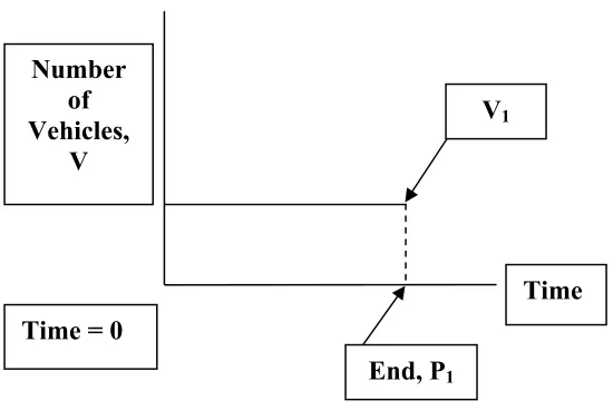
The first time period (P1) applies when the bus moves past the stop bar early in the

green phase starting when the effective green (g) equals zero. The ideal number of vehicles

is the amount that can traverse the intersection during the effective green time of the

intersection given no buses stopping during the signal cycle. Given an average vehicle

headway (h), this magnitude can be expressed as the effective green time (g) divided by the

(38)

the lane. Therefore, given the value of the bus blockage time (BT) and the vehicle headway

(h), the number of vehicles that are blocked can be calculated by dividing the blockage time

(BT) by the headway (h), or BT/h. However, vehicles can move past the stop bar as the

far-side bus stop is performed to fill the distance between the stop bar and the bus stop or to

make right-turns. Therefore, the number of vehicles that can get past the stop bar while the

bus is stopped is the number of storage spaces between the stop bar and the back of the bus

(St) divided by the proportion of through vehicles in the traffic stream (1 - Prt), where Prt is

the proportion of right-turns in the shared lane, St / (1 – Prt). Finally, we need to adjust for

time lost between when the bus finishes its stop and when the vehicles start flowing again.

This can be expressed as (L + h)/h, where ‘L’ is the lost time in seconds. Putting all of these

parts together, the average number of vehicles (V1) processed during the first time period (P1)

is computed by the following equation:

V1 = g/h – BT/h + St/(1-Prt) – (L + h)/h

The first time period ends at that time at which a stopped bus would start again, but

no more vehicles could be processed past the stop bar because the signal had turned red.

This time is (g – BT – (L + h)) which leads to the assumption that BT + L + h < g. A

(39)

Figure 1: Diagram of Time Period One (P1)

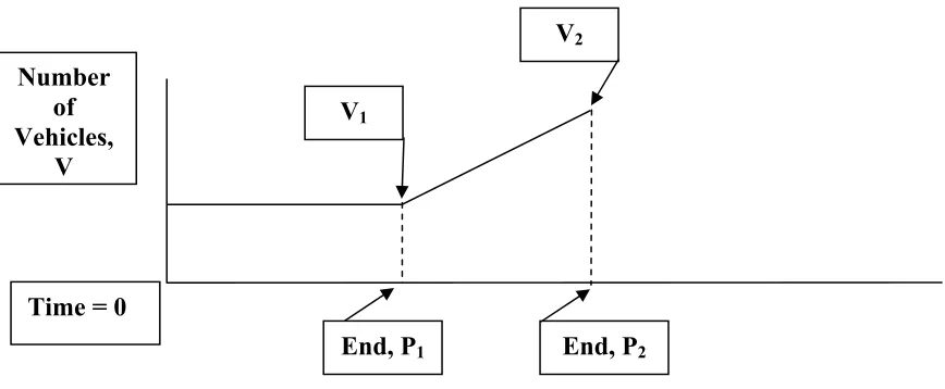
The second time period (P2) begins with the bus passing the stop bar at some point in

time greater than the value of (g – BT – (L + h)), or the end of P1. During P2, the storage

spaces behind the bus are filled so no more vehicles are processed by the travel lane, and the

bus does not start moving soon enough to allow vehicles to get beyond the stop bar because

the signal turns red. The number of vehicles that can be processed during a green phase

when a bus stops during P2 increases linearly during P2 from the number processed during P1

to the number processed during time period three, P3 (g/h, see below). The average number

of vehicles (V2) processed when a bus stops during P2 can be computed as:

V2 = (V1+ V3) / 2 =

(g/h – BT/h + St/(1-Prt) – (L + h)/h + g/h) / 2

P2 holds from the end of P1 at (g – BT – (L + h)), until the bus stop is no longer an issue to

the vehicles in the travel lane. This occurs at the time (g – (St * h)/(1 - Prt)). At that time and

for the rest of the effective green period, the storage spaces behind the stopped bus will not

fill up. Thus, the calculation of the length of P2 is as follows:

Number of Vehicles,

V

End, P1

Time = 0

V1

(40)

P2 = End of P2 – End of P1 = g – ((St * h)/(1 – Prt)) - (g – BT – (L + h)) =

BT – (St * h)/(1 – Prt) + L + h

A diagram of V2 and P2 is presented in Figure 2.

Figure 2: Diagram of Time Period Two (P2)

This leads to another assumption that BT + L + h > (St*h)/(1-Prt). During time period three

(P3), the bus stops so late in the green phase that the storage spaces are not filled before the

signal turns red.

With the bus stop no longer an issue, the number of vehicles that can be processed in

P3 by the travel lane is simply the ideal value of g/h. With the limit of the three distinct time

periods equal to the value of the effective green time, the length of P3 is calculated by

subtracting the beginning of P3 from the effective green time, g, as follows:

P3 = End of P3 – End of P2 = g - (g + (St * h)/(1 – Prt)) = (St * h)/(1 – Prt)

V

End, P1 End, P2

Time = 0

V1

(41)

With all time periods derived, the equation to obtain the average number of vehicles

processed during a green phase (VT) with a bus stop is as follows:

VT = (1 / g) * (V1 * P1 + V2 * P2 + V3 * P3)

In the preceding equation, P1, P2, P3, and g are calculated in seconds. Graphically, these

three distinct time periods are shown in Figure 3:

Figure 3: Diagram of All Three Time Periods

For example, if an effective green time of 40 seconds, a blockage time of 20 seconds, a

vehicle headway and lost time of 2 seconds each, a proportion of right turns at 0.50 (50%),

and 4 storage spaces are allowed behind a stopped bus, the average number of vehicles

expected for that cycle is computed as follows:

V1 * P1 = (40/2 - 20/2 + 4/(1-0.50) – (2+2)/2)*(40-20-2-2)

= (20 – 10 +8 – 2)*(40 – 20 – 4) = 256 veh-sec

V

Time

End, P1 End, P2

Time = 0

End, P3

V1

(42)

V1 * P1 = (g/h – BT/h + St/(1-Prt) – (L + h)/h + g/h)*(BT – (St * h)/(1 – Prt) + L + h)

= ((40/2 – 20/2 + 4/(1-0.50) – ((2+2)/2) + 40/2) * (20 – (4*2)/(1-0.50) + 2 + 2)

= ((40 – 10 + 8 – 2)/2)*(20 – 16 + 4) = 144 veh-sec

V3 * P3 = (g/h)*((St * h)/(1 – Prt)) = 40/2 * ((4*2)/(1-0.50))

= 20 * 16 = 320 veh-sec

VT =(1 / g) * V1 * P1 + V2 * P2 + V3 * P3

VT =40 * (256 + 144 + 320) = 18 vehicles per cycle containing a bus

With the average number of vehicles calculated, to obtain the saturation flow rate adjustment

for that cycle, the average number of vehicles (VT) is divided by the ideal number of vehicles

that can be processed by the intersection, g/h, which are 20 vehicles for this example.

Therefore, the adjustment factor is 18/20 or 0.90. This adjustment factor accompanied by an

adjustment factor for any cycles in an hour of analysis that does not contain a bus stop will

(43)

Chapter 5: Simulation Approach and Results

This chapter will address the process involved in creating and performing the

simulation runs that provide the data used to validate the equations derived in the last

chapter. The research relied upon CORSIM v. 5.1, a microscopic, stochastic simulation

package developed by the Federal Highway Administration (FHWA). With its established

track record, the ability to obtain and analyze results quickly, the ease in estimating

parameters, the ability to control the surrounding parameters, the ability to view simulations

in TRAFVU, and its ability to avoid the logistical difficulties that are encountered in

performing field experiments, the CORSIM simulation package was a good choice for this

research. Appropriate steps to ensure that CORSIM provides credible estimates of the

impact of bus stops on the saturation flow rate were followed.

When a traffic signal indication turns green, a separation between vehicles, or

headway, is introduced, measured in terms of seconds between consecutive vehicles crossing

the stop bar. If a consistent headway and a continuous green signal indication are observed

for a specified time period, e.g., a one-hour time period, a maximum theoretical flow rate is

expected. Any interruption in the green time will result in a capacity reduction. (4)

Method of Analysis

The research used CORSIM to model a saturated roadway network with one isolated,

pre-timed signalized intersection (Figure 4). Typical values regarding traffic signal timing

and roadway operations were assumed when needed. The entry number of vehicles per hour

(44)

reflect a saturated traffic condition. Efforts were made to view the simulations in TRAFVU

as well as examining the CORSIM output to verify the existence of a saturated flow

condition for each case simulated.

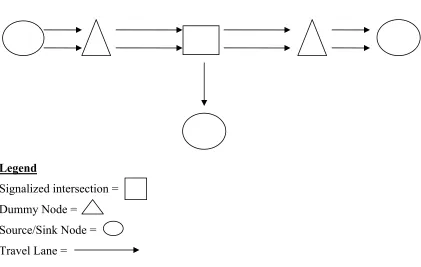
Legend

Signalized intersection = Dummy Node =

Source/Sink Node = Travel Lane =

Figure 4: Simulated CORISM Network

Each case simulated had two travel lanes: an exclusive through lane (CORSIM Lane

2) and a combination through-right turn lane (CORSIM Lane 1) that contained the curbside

bus stop. After the simulation runs were performed, data regarding the vehicle discharge for

the combination through-right turn lane was retrieved. By applying the amount of effective

green time and its proportion of the 60-minute simulation time period against the vehicle

(45)

is calculated. The discharge value for the combination lane already accounts for the effects

of the proportion of right-turns as well as the effects of the bus stops. For Lane 2, using the

proportion of the time period that is the effective green time and to the

discharge value, we can obtain a saturation flow rate. The inverse of this saturation flow rate

(3600 seconds / ideal flow rate) is calculated to obtain the headway per vehicle. Since Lane

2 did not contain any turn lanes, turning vehicles, or heavy vehicles and with all the

remaining details of Lane 2 having adjustment factors equal to 1.00, this calculated flow rate

value is referred to as the ‘ideal’ saturation flow rate per lane for each case.

The research consisted of two basic experiments – far-side and near-side bus stops.

For the far-side bus stop experiment, each simulation run was composed of a 60-minute time

period that is preceded by a warm-up (equilibrium) period not to exceed fifteen minutes. The

selection of a 60-minute time simplifies the subsequent calculations and allowed the

simulations to achieve stable operations. To obtain the saturation flow rate, output

referencing the vehicle discharge per lane, the average queue per lane, and the number of

buses serviced during the time period is utilized. Though additional performance data are

found in the CORSIM output, this research will only rely on select output that is used to

directly calculate the saturation flow rate.

In the experimental design, CORSIM requires the selected simulation time period be

evenly divisible by the traffic signal cycle length. If this situation does not exist, CORSIM

will revise the cycle length to a value that satisfies this constraint. To avoid any artificial

(46)

the 2000 HCM (pg. 16-160) suggests that to produce statistically significant values, a

minimum of fifteen complete signal cycles should be observed. Though CORSIM has the

ability to model actuated traffic signals, since each simulation contained a traffic volume that

sustained saturated conditions, actuated signals would behave like pre-timed traffic signals

anyway. Therefore, with each simulation having a 60-minute (3,600-second) time period, a

fixed cycle length of either 100 or 150 seconds that results in 24 to 36 complete signal cycles

per hour was used.

If a left-turn maneuver were introduced, to obtain any significant data, an opposing

traffic volume would need to be introduced into the simulation, thereby complicating the

research greatly. Therefore, with only traffic volumes simulated in a one-way direction, no

left-turning vehicles or maneuvers are included in this research. The remaining design

details listed below remained constant for all models. These values were also selected to

minimize any additional adjustment of the saturation flow rate:

a 90-degree intersection

free flow speed of 30 miles per hour

yellow and all red time of 4 seconds and 0 seconds, respectively lost time of 2 seconds

0% grade

Far-Side Bus Stop

Cases 1 – 12 modeled a basic roadway network with no buses with cases 13 to 17

modeling the far-side bus stop. With the high number of cases, only two repetitions of each

case were needed to provide adequate sample sizes. The two repetitions will use a different

set of random number seeds that were chosen from a spreadsheet of 8-digit random numbers

(47)

lane and a combination through-right turn lane and one pre-timed, signalized intersection.

The number of vehicles per hour necessary to sustain a saturated flow condition was selected

from a range of 1,000 to 2,500 vehicles per hour (vph). A 150-second signal cycle length

was selected that results in 24 complete signal cycles per simulation time period. Noting that

the effect of the far-side stop depends on the portion of the green phase in which the bus

arrives at the stop, four levels of effective green time (40, 60, 80, and 100 seconds) were

used. Three levels of right-turn percentage (0%, 12.5%, and 25% of the approach volume)

were selected. According to Chapter 16 of the HCM, the bus blockage factor measures the

effect of bus stops that occur within a 250-foot distance of the stop line. Therefore, bus stop

locations approximately 100 feet and 250 feet downstream of the stop line were modeled.

We could not make the bus stop any closer to the stop bar without the bus blocking part of

the cross street, which is not allowed in CORSIM. With the variability of the effective green

time and the restrictions on the far side analytical equation noted previously, only two levels

of bus dwell time (15 and 30 seconds) were modeled. Using a bus headway of 5 minutes

allows each bus and bus stop to remain independent of the preceding and proceeding one.

(48)

36

1 2 3 14a 14b 14c 14d 14e 14f 14g 14h 14i 14j 14k 14l

Right Turn % By Approach (veh) 0 12.5 25 0 12.5 25 0 12.5 25 0 12.5 25 0 12.5 25

Dwell Time (sec) 0 0 0 15 15 15 30 30 30 15 15 15 30 30 30

Bus Headway (minutes) 0 0 0 5 5 5 5 5 5 5 5 5 5 5 5

Bus Stop Distance from Stop Bar (feet) 0 0 0 100 100 100 100 100 100 250 250 250 250 250 250 Vehicles per hour (vph) 1000 1000 1000 1000 1000 1000 1000 1000 1000 1000 1000 1000 1000 1000 1000

60-Second Effective Green Case

4 5 6 15a 15b 15c 15d 15e 15f 15g 15h 15i 15j 15k 15l

Dwell Time (sec) 0 0 0 15 15 15 30 30 30 15 15 15 30 30 30

7 8 9 16a 16b 16c 16d 16e 16f 16g 16h 16i 16j 16k 16l

Dwell Time (sec) 0 0 0 15 15 15 30 30 30 15 15 15 30 30 30

10 11 12 17a 17b 17c 17d 17e 17f 17g 17h 17i 17j 17k 17l

Dwell Time (sec) 0 0 0 15 15 15 30 30 30 15 15 15 30 30 30