Estimation Method for First Excursion Probability of Secondary System with Impact and Friction Using Maximum Response

18th International Conference on Structural Mechanics in Reactor Technology (SMiRT 18) Beijing, China, August 7-12, 2005 SMiRT18-M04-7

ESTIMATION METHOD FOR FIRST EXCURSION PROBABILITY OF

SECONDARY SYSTEM WITH IMPACT AND FRICTION USING

MAXIMUM RESPONSE

Shigeru Aoki

Tokyo Metropolitan College of Technology

1-10-40 Higashi Ohi, Shinagawa-ku, Tokyo 140-0011, Japan

Phone: +81-3-3471-6331, Fax: +81-3-3471-6338

E-mail: [email protected]

ABSTRACT

The secondary system such as pipings, tanks and other mechanical equipment is installed in the primary system such as building. The important secondary systems should be designed to maintain their function even if they are subjected to destructive earthquake excitations. The secondary system has many nonlinear characteristics. Impact and friction characteristic, which are observed in mechanical supports and joints, are common nonlinear characteristics. As impact damper and friction damper, impact and friction characteristic are used for reduction of seismic response. In this paper, analytical methods of the first excursion probability of the secondary system with impact and friction, subjected to earthquake excitation are proposed. By using the methods, the effects of impact force, gap size and friction force on the first excursion probability are examined. When the tolerance level is normalized by the maximum response of the secondary system without impact or friction characteristics, variation of the first excursion probability is very small for various values of the natural period. In order to examine the effectiveness of the proposed method, the obtained results are compared with those obtained by the simulation method. Some estimation methods for the maximum response of the secondary system with nonlinear characteristics have been developed.

Keywords: Random vibration, Nonliear system, Seismic response, Response spectrum, Reliability

1. INTRODUCTION

The secondary system such as pipings, tanks and other mechanical equipment is installed in the primary system such as building. The important secondary systems should be designed to maintain their function even if they are subjected to destructive earthquake excitations. It is pointed out that seismic reliability of such important secondary system should be evaluated in probabilistic manner (Lin, 1967). First excursion failure is one of the most important failure modes (Lin and Cai, 1995) (Schueller, 1998). The secondary system has many nonlinear characteristics. Impact and friction characteristic, which is observed in mechanical supports and joints, are common nonlinear characteristics (Lin, 1991) (Abu-Yasein, Lay, Pickett, Madia and Sinha, 1997) (Aoki and Watanabe, 1998). As impact damper and friction damper, impact and friction characteristic are used for reduction of seismic response (Soong and Dargush, 1997).

modeled as single-degree-of-freedom system. As input ground motion, nonstationary artificial time histories compatible with the response spectrum are used. The Fokker-Planck equation is derived from equations of motion. The moment equations are obtained from integral of the Fokker-Planck equation. As impact characteristic, bilinear force-displacement relation is assumed. As friction characteristic, Coulomb friction is assumed. Friction force is equivalently linearized by considering stick and slip conditions. Even though input has Gaussian distribution, the response of the system with nonlinear characteristic has non-Gaussian distribution (Pradlwarter, 2001). Moments higher than second order are required to obtain the statistical characteristics of the nonlinear response (Bendat, 1990). However, Gaussian distribution of the response is assumed since statistical characteristics of the response are determined only from the second moments of the response. Under this assumption, the first excursion probability is obtained from the second moments of the response.

By using the methods, the effects of impact force, gap size and friction force on the first excursion probability are estimated. The first excursion probability decreases with the increase of impact force and with decrease of gap size. The first excursion probability decreases with the increase of friction force. When the tolerance level is normalized by the maximum response of the secondary system without impact or friction characteristics, variation of the first excursion probability is very small for various values of the natural period. The maximum response of the secondary system without impact or friction characteristics can be simply obtained by using some factors or modal analysis (Suzuki and Aoki, 1981) (Gupta, 1990). In order to examine the effectiveness of the proposed method, the obtained results are compared with those obtained by the simulation method. In general, the theoretical method gives larger value of the first excursion probability than the simulation method. A simple empirical equation which describes a relation between the tolerance level for the theoretical method and that for the simulation method is derived. Some estimation methods for the maximum response of the secondary system with nonlinear characteristics have been developed (Aoki and Suzuki, 1988), (Igusa and Sinha, 1991). Considering this point, the tolerance level is normalized by the maximum response of the secondary system with impact or friction. In those cases, variation of the first excursion probability is very small for various values of impact force, gap size and friction force.

It is concluded that when the tolerance level is normalized by the maximum response of the secondary system without impact or friction, the first excursion probability can be estimated independent of the natural period of the secondary system. It is also concluded that when the tolerance level is normalized by the maximum response of the secondary system with impact or friction, the first excursion probability can be estimated independent of impact force, gap size or friction force.

2. ANALYTICAL MODEL AND INPUT EXCITATION

As an analytical model, two-degree-of freedom model with impact or friction as shown in Fig.1(a) and Fig.1(b) are used. In this model, the secondary system and the primary system are modeled as single-degree-of-freedom system respectively. m is mass, c is damping coefficient, k is stiffness, x is absolute displacement. It is one of the model of secondary system with cap assuming mass ratio of the contacting system to the secondary system is negligible. Subscript s is used for the secondary system, p is for the primary system. And, y is absolute displacement of ground surface, d is gap size, kg is stiffness of collided part. fr is friction force. As input ground motion, artificial time histories compatible with the response spectrum is used. Figure 2 shows

(a) system with impact (b) system with friction

Fig.1 Analytical model with impact or friction

mp

m

s d

d

y _xp

cs

x s

kg

c p _kg

kp

ks

mp

m s f r f r

y _xp

cs

x s ks

target response spectrum (Japanese Ministry of International Trade and Industry, 1983). S is the response amplification factor, ratio of the maximum response of single-degree-of-freedom system to that of earthquake motion. Figure 3 shows envelope function I(t) representing nonstationary amplitude characteristic of earthquake motion (Jennings, Housner and Tsai, 1968).

3. ANALYTICAL METHOD FOR FIRST EXCURSION PROBABILITY

Theoretical method for obtaining the first excursion probability is shown. This method is based on the equivalent linearization method.

3.1 Equations of Motion 3.1.1 System with impact

Equations of motion with respect to relative displacement of the secondary system to the primary system zs and that of the primary system to the ground surface zp are written as:

(

)

_⎪⎭⎪⎬

⎫ − = + ω ζ γ − ω + ω ζ +

− − = + ω ζ +

y f z 2 z z

2 z

z y f z 2 z

1 s s s p 2 p p p p p

p 1

s s s s

(1)

where _⎟⎟

⎠ ⎞ ⎜⎜

⎝ ⎛ = ζ

mk 2

c

is the damping ratio, _⎟⎟ ⎠ ⎞ ⎜ ⎜ ⎝ ⎛ = ω

m k

is the natural circular frequency, _⎟⎟ ⎠ ⎞ ⎜ ⎜ ⎝ ⎛ = γ

p s

m m

is

mass ratio of the secondary system to the primary system. f is restoring force in the secondary system and has bilinear characteristic as shown in Figure 4. In this case, f is given as:

(

)(

)

(

)(

)

⎪ ⎪ ⎩ ⎪⎪ ⎨ ⎧

≤ +

+ ω + ω −

≤ ≤ − ω

≥ −

+ ω + ω =

d z : d z 1 b d

d z d : z

d z : d z 1 b d

f

s s

2 s 2 s

s s

2 s

s s

2 s 2 s

1 (2)

Fig.2 Target response spectrum Fig.3 Envelope function

Fig.4 Bilinear restoring force characteristic Fig.5 Coulomb friction characteristic

5

1

0.5

0.05 0.1 0.5 1 5

Natural Period(s)

S

0 0.2 0.4 0.6 0.8 1

0 10 20 30 40 50

t(s)

I(t) _{A B}

C OA:I(t)=t2/16

D AB:I(t)=1.0

BC:I(t)=exp{-0.0924(t-15)} CD:I(t)=0.05+0.005(50-t)2

f

xs f_r

ω_s2(b+1) f

xs 1

ω_s2 1 -d

d

1 eq

where b is stiffness ratio of collided part to the secondary system kg/ks. 3.1.2 System with friction

Equations of motion with respect to relative displacement of the secondary system to the primary system zs and that of the primary system to the ground surface zp are derived. When the secondary system moves to the primary system, equations of motion is given as:

(

)

_⎪⎭⎪⎬ ⎫ − = + ω + ω ζ γ − ω + ω ζ + − − = + ω + ω ζ + y f z z z z z z z z y f z z z z 2 s 2 s s s s p 2 p p p p p p 2 s 2 s s s s s (3)

where ζ

(

=c/

(

2 mk

)

)

is the damping ratio, ω

(

= k/m

)

is the natural circular frequency, γ

(

=ms/mp

)

is

mass ratio of the secondary system to the primary system, f is a term of friction characteristic. As friction characteristic, Coulomb friction characteristic as shown in Fig.5 is introduced. fr

(

=Fr/ms

)

is acceleration

corresponds to friction force. f is given as:

s s r 2 z z f f

= (4) Equation (3) is given when absolute acceleration of the primary system xp is greater thanfr. When this

condition is not satisfied, the condition where the secondary system does not move to the primary system should be considered. In this case,

0 zs =

and xs <fr (5)

where xs is absolute acceleration of the secondary system. And,

⎪ ⎭ ⎪ ⎬ ⎫ = = = st s s p s z z 0 z x x (6)

where zst is displacement when Eq.(6) is satisfied. The secondary system begins to move to the primary

system when each of the following equations is satisfied.

⎪ ⎭ ⎪ ⎬ ⎫ < > > < > ω + < < > > > ω − 0 x , 0 z or 0 x , 0 z ; f z x 0 x , 0 z or 0 x , 0 z ; f z x p st p st r st 2 s p p st p st r st 2 s p (7)

From Eq.(7), when the secondary system is subjected to earthquake motion from the condition z_s =0, the secondary system does not move to the primary system until the condition xp >fr is satisfied. Thus, fr is

determined by the maximum response of the linear system without friction characteristic

max p x _{as follows:} max p r x

f =ξ (8)

where ξ is normalized friction force and 0≤ξ≤1.

max p

x

_{is determined by multiplying S given by Fig.2 by}

the maximum ground acceleration

max g

x

.

3.2 Equation of first excursion probability

It is assumed that failure occurs when absolute value of displacement response of the secondary system zs

first crosses the tolerance levelBD. The first excursion probability Pf is obtained by the following equation

assuming Poison process (Soong and Grigoriu, 1992).

( )

⎭ ⎬ ⎫ ⎩ ⎨ ⎧_{− ν} −

=

∫

t

0 f(t) 1 exp 2 tdt

P (9)

When the probability density function is assumed to be Gaussian distribution,

ν

( )

t

is given as (Iyengar and Iyengar, 1970):

( )

{

( )

}

_⎥⎥ ⎦ ⎤ ⎢ ⎢ ⎣ ⎡ + ⎟ ⎟ ⎠ ⎞ ⎜ ⎜ ⎝ ⎛ σ − σ π κ + ⎪⎭ ⎪ ⎬ ⎫ ⎪⎩ ⎪ ⎨ ⎧ ⎟ ⎟ ⎠ ⎞ ⎜ ⎜ ⎝ ⎛ _κ + σ − σ π =

ν 1 erf C

2 B exp D 2 B D 1 2 B exp D 2 1 t ₂ z 2 D 2 z z z D 2 z z 2 z 2 D 2

z _{s s}

where

( )

∫

− π = κ − σ σ = σ = u 0 2 2 z z 2 z 2 z 2 z D z z dy y exp 2 ) u ( erf , D , D 2 B k C s s s s s s s (11) 2

σ and κ are variance and covariance for variable given by subscripts, respectively. 100 artificial time histories are generated (Vanmarcke, et al., 1968) and the expected value of power spectral density function of artificial time histories is obtained. In Fig. 6, the expected value is shown as broken line. The following equation (Tajimi, 1960) is fit to the expected value.

( )

(

)

(

)

(

)

0

2 g g 2 2 g 2 4 g 2 g g G 2 2 G ω ω ζ + ω − ω ω + ω ω ζ =

ω (12) where ζg is the damping ratio of the ground model,

g

ω is the natural circular frequency of the ground

model, G0 is power spectral density of white noise

which is input to the bed rock. Values of parameters, 5

. 0

g =

ζ ,Tg

(

=2π/ωg

)

=0.285s, G 1.94x10 (1/s)

3

0= − ,

give the best fit curve shown as solid line in Fig. 6. The Fokker-Planck equation of joint probability density function p with respect to relative displacement of the secondary system to the primary systemzs, relative

velocity zs , relative displacement of the primary

system to the ground zp, relative velocity zp, relative

displacement of the ground to the base rock z , relative g

velocity zg is expressed as (Aoki and Suzuki, 1985)

(Baratta, 1993):

(

)

{

( )

(

)}

(

)

(

)

(

)

(

)

{

}

(

)

2 G z p z z 2 z p p 2 z z p z z 2 f 1 z 1 z 1 2 z p p 1 2 z z p z z 2 t I f z z 2 z z 2 z p p 2 z z p t p 0 2 g 2 g 2 g g g g g g g g g p 2 p p p p s 2 s s s s s s s s s g 2 g g g g s 2 s s s s p 2 p p p p p p p p p π ∂ ∂ + ω + ω ζ ∂ ∂ + ω ζ + ∂ ∂ − ω + ω ζ + γ + − γ + ω − γ + ω ζ − ∂ ∂ − γ + ω ζ + ∂ ∂ − ω + ω ζ + + ω + ω ζ γ + ω − ω ζ − ∂ ∂ − ω ζ + ∂ ∂ − = ∂ ∂ (13) where I(t) is envelope function shown in Fig. 3. In order to use Eq.(4), the second moments with respect tozsand

s

z are to be obtained. Multiplying both sides of Eq.(6) by two state values, for examples, zs2,zszs,zszp so on,

and integrating from −∞ to ∞ with respect to zs,zs,z ,p zp,z andg zg, moment equations of second

moments with respect to zs,zs,z ,p zp,z andg zg are obtained as follows (Aoki, 1988).

p p p z z 2 z 2 dt d κ = σ s p p s s p z z z z z z dt d +κ κ = κ

(

)

_ps

( )

_ps

( )

_{p g}

p p s p p p p p z z g g z z 2 g z z eq s s z z p p z z 2 eq z 2 p 2 z z z t I 2 t I C 2 2 dt d κ ω ζ + κ ω + γκ + ω ζ + κ ω ζ − γκ ω + σ ω − σ = κ

Fig.6 Power spectral density function

(

)

_{p s pp}

(

)

(

)

_ps p s p s p z z eq s s z z p p z z 2 eq 2 z 2 p z z z z 1 C 2 2 1 dt d κ γ + + ω ζ − κ ω ζ + κ γ + ω − σ ω + κ = κ g p g p g p z z z z z z dt d +κ κ = κ g p g p g p g p z z g g z z 2 g z z z z 2 dt d κ ω ζ − κ ω − κ = κ

s _{s s} z z 2 z 2 dt d κ = σ

(

)

_ss

( )

_sg

( )

_{s g}

p s s s p s p p s z z g g z z 2 g z z eq s s z z p p 2 z 2 eq z z 2 p z z z z t I 2 t I C 2 2 dt d κ ω ζ κ ω + γκ + ω ζ + κ ω ζ − γσ ω + κ ω − κ = κ +

(

)

_{s s p}

(

)

(

)

_{s s}

s p s s s z z eq s s z z p p 2 z 2 eq z z 2 p 2 z z z 1 C 2 2 1 dt d κ γ + + ω ζ − κ ω ζ + σ γ + ω − κ ω + σ = κ g s g s g s z z z z z z dt d +κ κ = κ g s g s g s g s z z g g z z 2 g z z z z 2 dt d κ ω ζ − κ ω − κ = κ

p

{

_{pp ps s}

(

)

_{p s}

( )

_pg

( )

_{p g}

}

z z g g z z 2 g z z eq s s 2 z p p z z 2 eq z z 2 p 2 z t I 2 t I C 2 2 2 dt d κ ω ζ + κ ω + γκ + ω ζ + σ ω ζ − γκ ω + κ ω − = σ

(

)

( )

( )

(

)

_{p s p}

(

)

(

)

_ps

p p g s g s s s p s s s p s p z z eq s s 2 z p p z z 2 eq z z 2 p z z g g z z 2 g 2 z eq s s z z p p z z 2 eq z z 2 p z z 1 C 2 2 1 t I 2 t I C 2 2 dt d κ γ + + ω ζ − σ ω ζ + κ γ + ω − κ ω + κ ω ζ + κ ω + γσ + ω ζ + κ ω ζ − γκ ω + κ ω − = κ

(

)

( )

_g

( )

_{gg p g}

g 2 g p g s g p g p z z z z g g 2 z 2 g z z eq s s z z p p z z 2 eq z z 2 p z z t I 2 t I C 2 2 dt d κ + κ ω ζ + σ ω + γκ + ω ζ + κ ω ζ − γκ ω + κ ω − = κ

(

)

( )

_{g g}

( )

_{g pg pg}

g 2 g p g s g p g p z z g g z z 2 g 2 z g g z z 2 g z z eq s s z z p p z z 2 eq z z 2 p z z 2 t I 2 t I C 2 2 dt d κ ω ζ − κ ω − σ ω ζ + κ ω + γκ + ω ζ + κ ω ζ − γκ ω + κ ω − = κ

{

(

)

(

)

(

)

2

}

z eq s s z z p p z z 2 eq z z 2 p 2 z s s p s s s p

s _{2 1 2 2 C 1}

dt d σ γ + + ω ζ − κ ω ζ + κ γ + ω − κ ω = σ

(

)

_{s g p g}

(

)

(

)

_{2g s g}

g p g s z z z z eq s s z z p p z z 2 eq z z 2 p z z 1 C 2 2 1 dt d κ + κ γ + + ω ζ − κ ω ζ + κ γ + ω − κ ω = κ

(

)

_{s g pg}

(

)

(

)

_{2g sg sg}

g p g s z z g g z z 2 g z z eq s s z z p p z z 2 eq z z 2 p z z 2 1 C 2 2 1 dt d κ ω ζ − κ ω − κ γ + + ω ζ − κ ω ζ + κ γ + ω − κ ω = κ g g g z z 2 z 2 dt d κ = σ g g g g g g z z g g 2 z 2 g 2 z z z 2 dt d κ ω ζ − σ ω − σ = κ

(

)

0

2 z g g z z 2 g 2 z G 2 2 dt d g g g

g = −ω κ − ζ ω σ +π

σ

(14) For the system with friction, weq2 is given as Eq.(17) and for the system with friction, Ceq is given as Eq.(21).

3.3 Equivalent linearization method

3.3.1 Equivalent stiffness of system with impact

Nonlinear restoring force f is equivalently linearized as follows.

s eq

1 z

f =ω (15) where ωeq is the equivalent natural circular frequency. ωeq is approximately obtained by assuming stationary

random process since main shock is long. It is assumed that when amplitude of steady-state response to

harmonic excitation Zs is greater than d,

2 eq ⎟_⎠⎞ ⎜ ⎝ ⎛_ω ′

is approximately given as gradient of line connecting Zs and –Zs as shown in Fig. 4. Then,

(

)

⎪ ⎩ ⎪ ⎨ ⎧

≤ ω

> ω

− + ω = ⎟ ⎠ ⎞ ⎜ ⎝ ⎛_ω ′

d Z ;

d Z ; Z

d b Z 1 b

s 2 s

s s

2 s s 2

s 2

eq (16)

It is assumed that the probability density function of amplitude is Rayleigh distribution. The expected value

of

2 eq ⎟_⎠⎞ ⎜ ⎝ ⎛_ω ′

is obtained as:

( )

2 1

( )

1 s

1 2

s 2 s 2

eq b exp b erfc

− −

− _{− ω πη η}

η − ω + ω =

ω (17) where

d / 2

s z

σ =

η ,

∫

( )

−

π −

= u

0

2 _dy

y exp 2 1 ) u (

erfc (18)

3.3.2 Equivalent damping of system with friction Nonlinear force f is equivalently linearized as follows.

s eq 2 C z

f = (19) where Ceq is equivalent damping coefficient. It is assumed that friction force is not large and the secondary

system moves to the primary system near the main shock. And Ceq is approximately obtained by assuming

stationary random process since main shock is long. Equivalent damping coefficient for sinusoidal excitation is given as:

s i

r eq

Z f 4 ' C

πω

= (20)

where Zs is amplitude of steady-state response of the secondary system and ωi is frequency of excitation. It

is assumed that probability density function of amplitude is Rayleigh distribution. Expected value of C_eq' is obtained as:

s s

r eq

f 2 2 C

σ ω π

= (21)

eq

C near the main shock is given as Eq.(21). However, from the beginning of excitation to the main shock and after the main shock, Eqs.(5), (6) and (7) should be considered. From Eq.(7), when the system is subjected to excitation from equilibrium position, the secondary system moves to the primary system when xp >fr.

Considering this condition, Ceq is approximately obtained by using σx_p, standard deviation of xp. It is

assumed that standard deviation is proportional to the maximum response. First,

max x_p

σ , the maximum value of

standard deviation of linear system σx_p, is obtained. Next, it is assumed that when standard deviation of

absolute acceleration response of the primary system with friction σx_p is less than

max x_p

σ

ξ , Eqs.(5) and (6)

are satisfied with probability ps.

max x_p

σ

to response of the secondary system is 0 with probability ps. ps is approximately given as:

max x

x s

p p

p

σ ξ

σ

= (22)

When

max x x_p/ _p

ξσ

σ is less than 1, ps is assumed to be 0.

Fig.7 shows relation between psandσx_p. Second moments

with respect to response of the secondary system,σzs2, 2 zs

σ

and

s sz z

κ , are obtained by multiplying those obtained from

moment equations multiplying

{

}

2

max x xp/ p

ξσ

σ . Second

moments with respect to the secondary system and the primary system or the ground, for example κz_sz_p , are

obtained by multiplying those obtained from moment equations multiplying

max x xp/ p

ξσ

σ .

3. NUMERICAL EXAMPLES

Numerical results of the first excursion probability of the secondary system with impact are shown and the effect of collision on the first excursion probability is examined. Then, validity of obtained results is examined by simulation method.

3.1 Examples of system with impact 3.1.1 Gap Size and Tolerance Level

Gap size is normalized by the maximum response of the secondary system without impact

max z_s

z _A as:

max s *

z / d

d = A (23)

The tolerance level BD is normalized as:

max s D t =B /zA

δ (24)

max z_s

z _A is determined as:

2 s max p max

s Rx /

zA = ω (25)

where R is ratio of the maximum response of the secondary system without impact to that of the primary system.

max p

x is the maximum value of response of the primary system and given by S in Fig. 2. Some values of parameters are fixed as γ=0,

ζs=0.01 and ζp=0.05. For the natural period, the least feasible condition, that is Ts=Tp, is selected. In this case, response of the secondary system is greatly amplified. Values of the natural period are selected between 0.2s and 0.8s. In this condition, R in Eq.(25) is about 10 (Suzuki and Aoki, 1978). Pf is function of time. The important secondary system should maintain their functions after decaying earthquake excitation. In this paper, Pf after decaying earthquake excitation is obtained.

Fig.7 Relation between

ps

and

σx_p

Fig.8 First excursion probability of

secondary system with impact

(γ=0, ζs=0.01, ζp=0.05, Ts=Tp, b=5, d*=0.8)

ps

3.1.2 Obtained results

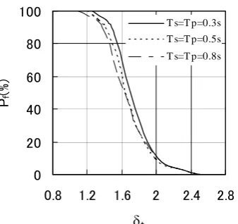
Figure 8 shows Pf for some values of the natural period. In this figure, b=5 and d*=0.8. Variation of Pf is very small. Same characteristic is obtained for other values of b and d*. Thus, Pf is independent of the natural period when the tolerance level is normalized as Eq.(24). And Pf for other values of the natural period can be obtained by using Figure 6.

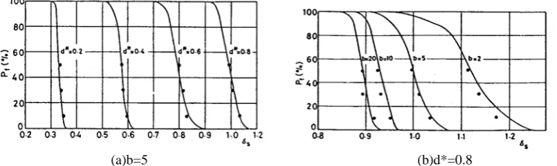
Next, the effect of d* and b on Pf is examined. Figure 9(a) shows Pf for some values of d*. In this figure, b=5. Figure 9(b) shows Pf for some values of b. In this figure, d*=0.8. From Fig.9(a), when d* is small, that means gap size is small, Pf is small. From Fig.9(b), when b is large, that means ratio of the stiffness of collided part to the secondary system is large, Pf is small. These figures show Pf for Ts=Tp=0.3s. From the results of Fig.8, Pf for other values of Ts=Tp can be estimated from Fig.9.

3.1.3 Simulation results

In order to examine validity of estimation method of Pf, Pf is obtained from simulation method using 100 artificial time histories. In order to distinguish from the tolerance level for theoretical method, symbol δs is used for the tolerance level for simulation method.

Figure 10 shows Pf for some values of the natural period. This figure corresponds to Figure 8. Variation of Pf is very small when the tolerance level is normalized as Eq.(24). This

(a)b=5 (b)d*=0.8

Fig.9 First excursion probability of secondary system with impact

(γ

=0,

ζ

s

=0.01,

ζ

p

=0.05, T

s

=T

p

)

Fig.10 First excursion probability of

secondary system with impact (simulation)

(γ=0, ζs=0.01, ζp=0.05, Ts=Tp, b=5, d*=0.8)

(a)b=5 (b)d*=0.8

characteristic is same as Figure 8.

Figure 11(a) shows Pf for some values of d*. In this figure, b=5. Figure 11(b) shows Pf for some values of b. In this figure, d*=0.8. These figures correspond to Figure 7. From Figure 11(a), when d* is small, Pf is small. From Figure 11(b), when b is large, Pf is small. When b is greater than 20, Pf is almost same as that for b=20. Thus, characteristic obtained from the proposed theoretical method is same as that from the simulation method.

Comparing Fig.8 with Fig.10 and Fig.9 with Fig.11, theoretical method gives larger values of Pf than simulation method. Main reason is that assumption used to obtain Eq.(9), time at which zs(t) crosses BD is statistically independent, is not strictly appropriate (Crandall and Mark, 1963). However, a simple relation between δt and δs can be obtained. The following equation between δt and δs is obtained by using least square method.

t 2 1 s =CC δ

δ (26) where

⎭ ⎬ ⎫ +

= + =

b 006 . 0 97 . 0 C

P 2 . 0 62 . 0 C

2

f 1

(27)

Pf obtained from Eq.(26) is shown in Fig.11 by dots. Obtained results well agree with those of simulation method qualitatively in the region in which Pf is relatively small.

3.2 Examples of System with Friction 3.2.1 Friction force and tolerance level

Friction force is determined as Eq.(8). The tolerance level BD is normalized by the maximum response of the secondary system without friction zsA_maxas same as Eq.(24).

Some values of parameters are fixed as γ=0, ζs=0.01 and

ζp=0.05. For the natural period, the least feasible condition, that is Ts=Tp, is selected. In this case, response of the secondary system is greatly amplified. Values of the natural period are selected between 0.3s and 0.8s. Pf is function of time. The important secondary system should maintain their function after earthquake excitation. In this paper, Pf after earthquake excitation is obtained.

3.2.2 Obtained results

Figure 12 shows Pf for some values of the natural period. ξ is fixed as 0.05. Variation of Pf is very small. Same characteristic is obtained for the case where ξ is less than about 0.1 Thus, Pf is independent of the natural period when the tolerance level is normalized as Eq.(24).

Figure 13 shows Pf for some values of ξ. From this figure, when ξ is large, that means friction force is large, Pf is small. This figure shows Pf for Ts=Tp=0.3s. From the results of Fig.12, Pf for other values of Ts=Tp is obtained from Fig.13.

3.2.3 Simulation results

In order to examine validity of estimation method of Pf, P is obtained from simulation method using 100 artificial time histories. In order to distinguish from the tolerance level for theoretical method, symbol is used for the tolerance level for simulation method.

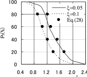
Figure 14 shows Pf for some values of ξ. This figure corresponds to Fig.13. In Fig.14, when ξ is large, that means friction force is large, Pf is small. This characteristic corresponds to Fig.13. Thus, characteristic obtained from the proposed theoretical method is same as that from the simulation

Fig.12 First excursion probability of

secondary system with friction

(γ=0, ζs=0.01, ζp=0.05, Ts=Tp, ξ=0.05)

Fig.13 First excursion probability of

secondary system with friction

(γ=0, ζs=0.01, ζp=0.05, Ts=Tp)

0 20 40 60 80 100

0.8 1.2 1.6 2 2.4 2.8

δt

Pf

(%

)

T s=T p=0.3s

T s=T p=0.5s

T s=T p=0.8s

0 20 40 60 80 100

0.8 1.2 1.6 2 2.4 2.8

δt Pf

(%

)

method. Comparing Fig.13 with Fig.14, theoretical method generally gives larger values of Pf than simulation method. The reason is that assumption used to obtain Eq.(7), time at which zs(t) crosses BD is statistically independent, is not strictly appropriate (Crandall and Mark, 1963). However, a simple relation between δt and δs can be obtained. The following equation between δt and δs is obtained by using least square method.

δs =δt/

{

(

2−Pf

)(

1.1−ξ

)

}

(28)

Pf obtained from Eq.(28) is shown in Fig.14 by dots. Obtained results well agree with those of simulation method qualitatively.

4. ESTIMATION METHOD USING NONLINEAR RESPONSE

In chapter 3, estimation method of Pf using the maximum response of the secondary system without impact as Eg.(24) is shown. In this chapter, estimation method using the maximum response of the secondary system with impact or friction is proposed.

4.1 System with Impact

For example, we focused on Pf for d*=0.8. Tolerance level for Pf=0.5, which is considered as the expected value of the response, is defined as δs*. For Pf=0.5, comparing the tolerance level for other than d*=0.8 with that for d*=0.8, the following equation is obtained.

* C_{3 s}

s = δ

δ (29) Figure 15 shows C3. The tolerance level for Pf for other than Pf=0.5 is obtained using Figure 15 and Eq.(29). Results are shown

as ▲ in Fig.16. Results obtained by Eq.(29) agree with those obtained by simulation method shown as solid lines. This method is applied to the results obtained by theoretical method shown in Figure 11(a). Results are shown as ▲ in Fig.17. Results obtained by Eq.(14) agree with those obtained by theoretical method shown as solid lines. Thus, when Pf is obtained for one value of d* (for example d*=0.8), Pf for other values of d* can be estimated by Eq.(14). δs* corresponds to the expected value of the maximum response of the secondary system with impact. Estimation methods of the maximum response of the secondary system with nonlinear characteristics have been developed [9],[10]. Thus, Pf can be obtained form Eq.(14) using the maximum response of the secondary system with nonlinear characteristics.

4.2 System with Friction

Fig.14 First excursion probability of

secondary system with impact (simulation)

(γ=0, ζs=0.01, ζp=0.05, Ts=Tp)

Fig.15 Value of C

3

Fig.16 First excursion probability of

secondary system with impact (simulation)

(γ=0, ζs=0.01, ζp=0.05, Ts=Tp, b=5)

Fig.17 First excursion probability of

secondary system with impact

(γ=0, ζs=0.01, ζp=0.05, Ts=Tp, b=5)

0 20 40 60 80 100

0.4 0.8 1.2 1.6 2.0 2.4

δs

P

f

(%

)

ξ=0.05 ξ=0.1

In Eq.(17), the tolerance level is normalized by the maximum response of the secondary system without friction. In this chapter, an estimation method of the first excursion probability using the maximum response of the secondary system with friction is proposed.

The tolerance level BD is normalized by the maximum response of the secondary system with friction zsf _maxas same

as Eq.(28).

max sf D t*=B /z

δ (30)

max sf

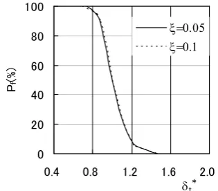
z is determined as the expected value of the maximum response of the secondary system with friction which is assumed to be the tolerance level for Pf=0.5 in Fig.13. Figure 18 shows the result obtained from Fig.13 using Eq.(30). Variation of Pf for ξ is very small.

For simulation results, BD is normalized as Eq.(30). max

sf

z is assumed to be the tolerance level for Pf=0.5 in Fig.14. Symbol s is used. Fig.19 shows the result. In this case, Variation of Pf for ξ is very small.

ξ defined as Eq.(8) corresponds to the friction force. Thus, Pf is independent of the friction force when the tolerance level is normalized by the maximum response of the secondary system with friction as Eq.(30).

5. CONCLUSIONS

An estimation method of the first excursion probability of the secondary system with impact or friction subjected to earthquake excitation is proposed. In this method, the maximum response is used.

For the system with impact, a theoretical estimation method for the first excursion probability of the secondary system is proposed. Using this method, the effect of gap size and stiffness ratio of collided part to the secondary system on Pf is examined. Next, obtained results are shown by normalizing the tolerance level by the maximum response of the secondary system. Obtained results are summarized as follows:

(1) When the tolerance level is normalized by the maximum response of the secondary system without impact, elastic system, as Eq.(24), variation of Pf is very small for various values of the natural period.

(2) Pf becomes small with the decrease of gap size. Pf becomes small with the increase of stiffness ratio of collided part to the secondary system b.

(3) Theoretical method gives greater value of Pf than simulation method. Equation (26) gives relation between the tolerance level for theoretical method and that for simulation method.

(4) Using Pf for one value of nonlinear parameter and Eq.(29), Pf for other values of nonlinear parameter can be estimated.

For the secondary system with friction, obtained results are summarized as follows:

(1) The tolerance level is normalized as Eq.(24), variation of Pf is very small for various values of the natural period.

(2) Pf becomes small with the increase of friction force.

(3) In general, theoretical method gives greater value of Pf than simulation method. Equation (28) gives relation between the tolerance level for theoretical method and that for simulation method.

(4) Using Pf for one value of nonlinear parameter and Eq.(30), Pf for other values of nonlinear parameter can be estimated.

Fig.18 First excursion probability of

the secondary system using

normalized tolerance level as Eq.(30)

(

γ

=0,

ζ

_s=0.01,

ζ

_p=0.05,Ts=Tp=0.3s)

Fig.19 First excursion probability of the

secondary system using normalized

tolerance level as Eq.(30) (simulation)

(

γ

=0,

ζ

_s=0.01,

ζ

_p=0.05,Ts=Tp=0.3s) 0

20 40 60 80 100

0.4 0.8 1.2 1.6 2.0

δt*

P

f

(%)

ξ=0.05 ξ=0.1

0 20 40 60 80 100

0.4 0.8 1.2 1.6 2.0

δs*

P

f

(%

)

REFERENCES

Abu-Yasein, OA., Lay, C., Pickett, M.A., Madia, J., Sinha, S.K., (1997), The Influence of Higher Modes and Support Gaps on the Seismic Response of Piping Systems Containing Snubbers. Transactions of ASME, Journal of Pressure Vessel Technology, Vol.119, No.4, pp.444-456

Aoki, S., Suzuki, K., (1985), First Excursion Probability Estimation of Mechanical Appendage System Subjected to Nonstationary Earthquake Excitations, Proceedings of the 4th International Conference on Structural Safety and Reliability, Vol.I, pp.201-210

Aoki, S., Suzuki, K., (1988), Dynamic Response Reduction Effect of the Piping due to Gap and Friction. Proceedings of the ASME Pressure Vessels and Piping Conference, Application of Modal Analysis to Extreme Loads, PVP-150, pp.17-21

Aoki, S., (1988), First Excursion Probability of Secondary System Subjected to Earthquake Excitations. Report of Tokyo Metropolitan College of Technology, No.23, pp.1-8

Aoki, S., Watanabe,T., (1998), Forced Vibration of Continuous System with Unsymmetrical Collision Characteristics, Nonlinear Dynamics, Vol.17, pp.141-157

Baratta, A., (1993), Dynamic Motion Chaotic and Stochastic Behaviour, Approximate Solution of the Fokker-Planck-Kolmogorov Equation for Dynamical Structure, Dynamic Motion Chaotic and Stochastic Behaviour Edited by Casciati,F., Springer-Velag, New York, pp.93-125

Bendat, J.S. (1990), “Nonlinear System Analysis & Identification”, John Wiley & Sons, New York, 15-73 Clough, R.W., Penzien, J., (1993), “Dynamics of Structures (Second Edition)”, McGraw-Hill, Singapore, pp.575-611

Crandall,S.H. and Mark,W.D., (1963), “Random Vibration in Mechanical System”, Academic Press, New York, pp.106-110

Gupta, A.K., (1990), “Response Spectrum Method”, Blackwell Scientific Publications, Cambridge, pp.89-124 Igusa, T., Sinha, R., (1991), Response Analysis of Secondary System with Nonlinear Supports. Transactions of ASME, Journal of Pressure Vessel Technology, Vol.113, No.4, pp.524-531

Iyengar, R.N., Iyengar, K.T.S.R., (1970), Probabilistic Response Analysis to Earthquakes. ASCE Journal of Engineering Mechanics Division, Vol.96, No.3, pp.207-225

Japanese Ministry of International Trade and Industry. (1983), Guidelines for Aseismic Design of High Pressure Gas Facilities

Jennings, P.C., Housner, G.W., Tsai, N.C., (1968), Simulated Earthquake Motions. Earthquake Engineering Research Laboratory, California Institute of Technology, pp.7-8

Lin, C.W., (1991), Seismic Evaluation of System and Components. Transactions of ASME, Journal of Pressure Vessel Technology, Vol.113, No.2, pp.273-283

Lin, YK., (1967), “Probabilistic Theory of Structural Dynamics”, Krieger, New York, pp.293-338 Lin, Y.K., Cai, G.Q., (1995), “Probabilistic Structural Dynamics”, McGraw-Hill, Singapore, pp.363-404

Pradlwarter,H.J. (2001), “Non-Gaussian Response Distributions of Non-linear MDOF- systems”, Proceedings of the Eighth International Conference on Structural Safety and Reliability, CD-ROM

Schueller, G.I., (1998), Structural Reliability –Recent Advances. Proceedings of the 7th International Conference on Structural Safety and Reliability, Vol.1, pp.3-35

Soong, T.T., Dargush, G.F., (1977), “Passive Dissipation Systems in Structural Engineering”, John Wiley & Sons, Chichester, pp.83-126

Soong,T.T. and Grigoriu, M., (1992), Random Vibration of Mechanical and Structural Systems, Prentice Hall, Englewood Cliffs, 305-306

Suzuki K., Aoki, S., (1981), Conventional Estimating Method of Earthquake Response of Mechanical Appendage System Installed in the Nuclear Structural Facilities. Transactions of the 6th International Conference on Structural Mechanics in Reactor Technology, K10/3, pp.1-8

Tajimi, H., (1960), A Statistical Method of Determining the Maximum Response of a Building Structure during an Earthquake, Proc. 2nd World Conference on Earthquake Engineering, Vol.II, pp.781-798