Some Numerical Results on Function Space (Fsa) Algorithms

(1)

504

SOME NUMERICAL RESULTS ON FUNCTION SPACE (FSA) ALGORITHMS

J. O. Omolehin1 K. Rauf2 A. Mabayoje3 O. T. Arowolo4 A. Lukuman5

ABSTRACT

In this work, we consider the numerical implementation of Function Space Algorithm (FSA) for the solution of quadratic continuous cost functional. It is used to solve Reaction Diffusion Control problems. It considered specifically a parabolic problem characterized by dynamics constraints and the results obtained analyzed. The cumbersome nature of the line search techniques associated with FSA was addressed by time discretization approach. It is shown that the convergence rate of FSA improves as the penalty parameter grows.

Key Words:FSA, Penalty parameter, Constraints, Convergence rate, Time Discretization

2010 Mathematics Subject Classification: 93B40, 93CXX & G 1.7

INTRODUCTION

Let us first consider the quadratic functional of the form:

Where is an 𝑛𝑥𝑛 symmetric positive definite matrix operator on the Hilbert space 𝐻. 𝛼 is a vector in 𝐻 and 𝐹0 is a constant term.

1_{Mathematics and Computer Science Department, IBB University, Lapai, Nigeria}

2_{Mathematics Department, University of Ilorin, Ilorin, Nigeria}

3

Computer Science Department, University of Ilorin, Ilorin, Nigeria

4_{Mathematics and Statistics Department, Lagos State Polytechnics, Lagos State}

5

Federal College of Fisheries and Marine Technology, Lagos State

 

,

2

1 ,

H H

o

a

x

Ax

F

x

F















A

Journal of Asian Scientific Research

(2)

505

Let us also consider what is termed conjugate descent with 𝐹. With conjugate descent, it is

assumed that a sequence

𝑝𝑖 = 𝑝0, 𝑝1, … , 𝑝𝑘, ..

is available with the members of the sequence conjugate with respect to the positive definite linear

operator .

By conjugate with respect to 𝐴, we mean that

< 𝑝𝑖, 𝐴𝑝𝑖 >𝐻= ≠ 0, 𝑖𝑓 𝑖 ≠ 𝑗_{= 0, 𝑖𝑓 𝑖 = 𝑗}

In this case, 𝐴 is assumed positive definite so < 𝑝𝑖, 𝐴𝑝𝑖>𝐻> 0.

The conventional Conjugate Gradient Method (CGM) was originally designed for the minimization of a quadratic objective functional of the form stated above.

STAGES INVOLVED IN CONJUGATE GRADIENT METHOD

Stage 1: The first element 𝑥0∈ 𝐻 of the descent sequence is guessed while the remaining members

of the sequence are computed with the aid of the following formulae:

Stage 2: 𝑝0= −𝑔0= −(𝑎 + 𝐴𝑥0)

(𝑝0 is the descent direction and 𝑔0 is the gradient of 𝐹(𝑥) when 𝑥 = 𝑥0)

Stage 3: 𝑥𝑖+1= 𝑥𝑖+ 𝛼𝑖𝑝𝑖, 𝛼𝑖 =< 𝑔𝑖, 𝑔𝑖>𝐻/< 𝑝𝑖,𝐴𝑝𝑖>𝐻

𝛼 is the step length

Stage 4: if 𝑔𝑖 for some 𝑖 terminate the sequence else, set 𝑖 = 𝑖 + 1 and go to stage 3.

The CGM has a well worked out theory with an elegant convergence profile. It has been proved that the algorithm converges, at most, in n iterations in a well posed problem and the convergence

rate is given as:

A

;

1 i i i

i

g

a

Ap

g

_





H i i H i i i i i i

i

g

p

g

p

_₁





_₁





;





_₁

,

_₁



/



,



   0

2

1 1

x E

M m M m

x E

n

      

      

(3)

506

Where m and M are smallest and spectrums of matrix A respectively

That is, for an n dimensional problem, the algorithm will converge in at most n iterations.

The CGM algorithm cannot handle quadratic cost functional of the form:

Minimise

Subject to

𝑣 = 𝑐𝑣 𝑡 + 𝑑𝑢(𝑡)

For the reason that operator A was not known explicitly in continuous cost functional, researchers

came up with different approximation – based techniques that could estimate 𝛼𝑖 that minimizes F(xi

+ αpi). (1) In this fashion, there came into being various cumbersome techniques. The most popular

among such methods is the conventional function space (CFS) algorithm, (1) to minimize the

continuous cost functional of the form:

Problem (1)

Minimise 𝑥_𝑜𝛿 𝑇 𝑡 𝑄𝑥 𝑡 + 𝑢𝑇 𝑡 𝑃 𝑢 𝑡 𝑑𝑡

Subject to the dynamic constraints

𝑥 (t) =C x (t) + Du (t),

0 < t < δ (δ given); where 𝑥(t) denotes the transpose of x(t), 𝑥 (t) stands for the first derivative of x(t) with respect to t. x(t) is the n x 1 state vector, u(t) is the q x 1 control vector, C and D are n x q

constant matrices respectively, while Q and R are symmetric, positive definite, constant square matrices of dimensions n and q respectively.

The control operator A is associated with problem (1) satisfying

< 𝐴, 𝐴𝑍 > K= J x, u,μ = {xT δ

0

t Qx t + u(t)T_Pu(t)

+μ|| 𝑥 (t) – Cx(t) – Du(t) ||2_}dt₍_μ_{> 0)}

by transforming problem (1) into an unconstrained optimal control problem. Where μ is the penalty constant 𝐾 is given by K = 𝐻1[0, δ] x Lq2 [0, δ], and 𝐻1 [0, δ], denotes sobolev space of the

absolutely continuous functions x(.), square integrable over the closed interval [0, δ].

 









T

dt

t

bu

t

av

0

(4)

507 𝐿𝑞₂ 0, 𝛿 stands for the Hilbert space consisting of the equivalence classes of square integrable functions from [0, δ] into Rq, with norm denoted by ||. ||𝐸 and defined by

| | u | | = {||u||2} 1 2 𝑑𝑡

𝛿

0 and with scalar product conventionally denoted by < .,.> and defined by

<u1, u2> = < u₀δ 1, u2 >E dt where ||. ||𝐸 and <. , . >𝐸 denote the norm and scalar product in

Euclidean q – dimensional space.

FUNCTION SPACE ALGORITHM

The function space algorithm is constructed to solve the optimal control problem (1):

Min J (x, u, μ) = Min {x𝑅 T_{(t) Px (t) + u}T_{(t) Qu(t) } dt} 0

+μ | |(x (t) – Cx(t) – Du(t) || ₀T 2dt

Where C and D are constant matrices of appropriate dimensions. The steps involve in FSA is as follows:

Step 1

choose the initial values x 0 t , uo t ,

where 0 < 𝑡 < 𝑇, 𝑇 𝑖𝑠 𝑘𝑛𝑜𝑤𝑛 𝑎𝑛𝑑 𝑐𝑜𝑚𝑝𝑢𝑡𝑒 xo t = x 0 t T

o

dt

Step 2

Initialize the Counter: i = 0, and compute [∇_xJ ]i, ∇U J

i using formulae for

∇J = ∇X J

∇_UJ

∇_XJ = 2μ x t − f x(t , u t , t ] − (t ∂T_∂x)T T –

∂f ∂x

T

[2μ(x s − f(x s , u(s), s)] }ds

0 < t < T

[∇uJ] = ∂I ∂u − (

∂F ∂v)

(5)

508 Step 3

Compute the current descent direction.

s x,i 𝑡 = { _{− ∇}

𝑋 𝐽_{𝑖 + 𝛽}

𝑖−1𝑆 𝑋 ,𝑖−1 𝑡 , 𝑓𝑜𝑟 𝑖>0,𝑤𝑕𝑒𝑟𝑒 𝑡 ∈ 𝑜,𝑇

{− ∇ 𝑜, 𝑓𝑜𝑟 𝑖=𝑜

sx,i (t) = 𝑠 𝑥,𝑖(𝑡) 𝑡

𝑜 𝑑𝑡

s u,i(𝑡) = { _{− ∇}

𝑈 𝐽

𝑖 + 𝛽𝑖−1𝑆𝑖−1 𝑡 𝑓𝑜𝑟 𝑖>0

{− ∇_𝑈𝐽

0 , 𝑓𝑜𝑟 𝑖=𝑜

Where t [0, T ], and

𝛽𝑖−1=

|| ∇𝑥𝐽 _𝑖||2 𝑑𝑡 + 𝑇

𝑜 || ∇𝑢𝐽 _𝑖||2 𝑑𝑡

𝑇 𝑜 || ∇𝑥𝐽 𝑖−1||2 𝑑𝑡 +

𝑇

𝑜 || ∇𝑢𝐽 𝑖−1||2 𝑑𝑡

𝑇 𝑜

STEP 4

Find P*i

such that J (xi + Pi* sx, i, ui + P*i su,i, μ,) < J (xi + pi sX, i ui + pi su,i, μ,), p>o

STEP 5

Test for the stopping criterion of the algorithm by verifying if

S(x, u, μ) = || Ø (z) ||2

+ ( Jx )T ( Jx) + ( uJ) T ( uJ) < ε,

(Ø = 𝑥 - f)

Where ε is a chosen predetermined tolerance to indicate that the desired accuracy required for the computational programming method.

STEP 6

Set 𝑥𝑖+1(t) =𝑥 𝑖(t) +𝑝 ∗𝑖s (t) 0 <t< T

𝑢𝑖+1(t) =𝑢 𝑖(t) +𝑝 ∗𝑖s (t) 0 <t< T

STEP 7

(6)

509

To the best knowledge of the authors, no numerical work has been carried out prior to the time this

work was concluded.

NUMERICAL RESULTS ON FSA

In carrying out our numerical investigation using FSA algorithm discussed, we study computationally the convergence rate of various diffusion equation problems which are only dimensionally different from one another. Thus, when we say the dimensionality of the resulting

diffusion control problem is ℝ12 and ℝ11 it means that is α, u ∈ ℝ12 and

α, u ∈ ℝ11_{, respectively.}

Thus, in ℝ12 and ℝ11we have problems (1) and (2) respectively as stated below:

Problem (1)

Minimize {𝛼12 𝑡 + 𝛼22 𝑡 + … + 𝛼122 𝑡 + 𝑢12 𝑡 + 𝑢22 𝑡 + … + 1

𝑜 𝑢12 2 𝑡 }𝑑𝑡

Subject to α1 (t) = -π2α1 (t) + u1 (t)

α2 (t) = -4π2α2 (t) + u2 (t)

……….

α12 (t) = -144π2α12 (t) + u12 (t)

The problem is transformed into an unconstrained problem with the introduction of a penalty constant μ and it becomes:

Min J (α, u, μ) = Min {𝛼_𝑜1 12 𝑡 + 𝛼2 2 𝑡 + … + 𝛼122 𝑡 + 𝑢1 2(t) + 𝑢22 𝑡 + … + 𝑢12 2 𝑡 ] 𝑑𝑡

+ 𝜇{ { 𝛼1(𝑡) + 𝜋2𝛼1 𝑡 − 𝑢1(𝑡) 2

+ 𝛼2(𝑡) + 4𝜋2𝛼2 𝑡 − 𝑢2(𝑡) 2

+ 𝛼3(𝑡) + 9𝜋2𝛼3 𝑡 − 1

0

𝑢3(𝑡)2+…+𝛼12(𝑡)+144𝜋2𝛼12𝑡−𝑢12(𝑡)2}}dt

Also, problem in ℝ11 i.e. when α, u ℝ11, we obtain the following equivalent problem

formulation:

Problem (2)

Minimize {𝛼_𝑜1 12 𝑡 + 𝛼22 𝑡 + … + 𝛼112 𝑡 + 𝑢12 𝑡 + 𝑢22 𝑡 + … +𝑢11 2 𝑡 𝑑𝑡

(7)

510

α1 (t) = -π2α1 (t) + u1 (t)

α2 (t) = -4π2α2 (t) + u2 (t)

……….

α11 (t) = -122π2α11 (t) + u11 (t)

The problem is now transformed into an unconstrained problem with the introduction of a penalty constant μ.

Min J (α, u, μ) = Min {𝛼_𝑜1 12 𝑡 + 𝛼2 2 𝑡 + … + 𝛼112 𝑡 (𝛼, 𝑢)

+ 𝑢1(t) + 𝑢22 𝑡 + … + 𝑢11 2 𝑡 ] 𝑑𝑡 + 𝜇{ { 𝛼1(𝑡) + 𝜋2𝛼1 𝑡 − 𝑢1(𝑡) 2

+ 1

0

𝛼2(𝑡)+4𝜋2𝛼2𝑡−𝑢2(𝑡)2+𝛼3(𝑡)+9𝜋2𝛼3𝑡−𝑢3(𝑡)2+…+𝛼11(𝑡)+121𝜋2𝛼11𝑡−𝑢11(𝑡)2}}dt.

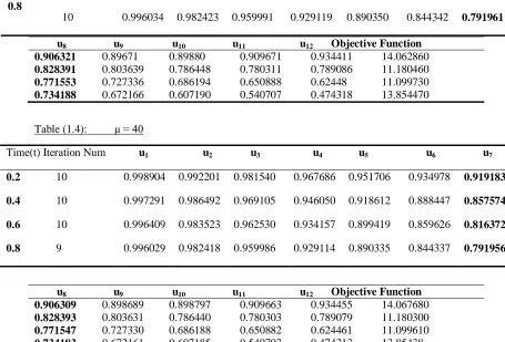
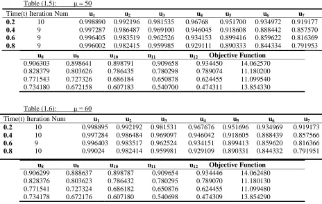
The problems in other dimensions can easily be formulated in similar manner. Meanwhile, the convergence rate for various values of penalty constants in ℝ12 is shown by Tables (1.1) – (1.6).

Table-1. FSA Algorithm in ℝ𝟏𝟐

Table (1.1): μ = 10

Time (t)Iteration Num u1 u2 u3 u4 u5 u6 u7

0.2

0.4

0.6

0.8

4

9

8

0.998991

0.997361

0.996464

0.996073

.992290

0.986562

0.983578

0.982462

0.981630

0.969175

0.962585

0.960030

0.967777

0.94612

0.934212

0.929157

0.951799

0.918683

0.899475

0.890379

0.935071

0.888516

0.859680

0.844381

0.919281

0.857644

0.816428

0.79200

u8 u9 u10 u11 u12 Objective Function

0.906385 0.828453 0.771602 0.734227

0.898730 0.803700 0.727384 0.672205

0.898913 0.786510 0.686244 0.607229

0.909716 0.780373 0.650937 0.540747

0.934522 0.789148 0.624517 0.474358

(8)

511

Table (1.2): μ = 20

Time (t)Iteration Num u1 u2 u3 u4 u5 u6 u7

0.2 0.4 0.6 0.8 5 8 9 10 0.998933 0.997315 0.996427 0.996044 0.992232 0.986516 0.983541 0.982433 0.981572 0.969129 0.962549 0.960001 0.967719 0.946074 0.934175 0.929128 0.951742 0.918636 0.899438 0.890350 0.935017 0.888471 0.859644 0.844352 0.919213 0.857598 0.816391 0.791971

0.906306 0.828406 0.771565 0.734198 0.898689 0.803654 0.727347 0.672176 0.898843 0.786463 0.686207 0.607200 0.909705 0.780326 0.650901 0.540718 0.934476 0.789102 0.624480 0.474329 14.063360 11.180790 11.099970 13.854660

Table (1.3): μ = 30

Time(t) Iteration Num u1 u2 u3 u4 u5 u6 u7

0.2 0.4 0.6 0.8 4 9 10 10 0.998914 0.997299 0.996415 0.996034 0.992212 0.986500 0.983529 0.982423 0.981552 0.969113 0.962536 0.959991 0.967699 0.946058 0.934163 0.929119 0.951722 0.918620 0.899426 0.890350 0.934990 0.888455 0.859632 0.844342 0.919200 0.857582 0.816378 0.791961

0.906321 0.828391 0.771553 0.734188 0.89671 0.803639 0.727336 0.672166 0.89880 0.786448 0.686194 0.607190 0.909671 0.780311 0.650888 0.540707 0.934411 0.789086 0.62448 0.474318 14.062860 11.180460 11.099730 13.854470

Table (1.4): μ = 40

0.906309 0.828393 0.771547 0.734183 0.898689 0.803631 0.727330 0.672161 0.898797 0.786440 0.686188 0.607185 0.909663 0.780303 0.650882 0.540703 0.934455 0.789079 0.624461 0.474313 14.067680 11.180300 11.099610 13.85438

(9)

512

Table (1.5): μ = 50

0.2 0.4 0.6 0.8 10 9 9 9 0.998890 0.997287 0.996405 0.996002 0.992196 0.986487 0.983519 0.982415 0.981535 0.969100 0.962526 0.959985 0.96768 0.946045 0.934153 0.929111 0.951700 0.918608 0.899416 0.890333 0.934972 0.888442 0.859622 0.844334 0.919177 0.857570 0.816369 0.791953

0.906303 0.828379 0.771543 0.734180 0.898641 0.803626 0.727326 0.672158 0.898791 0.786435 0.686184 0.607183 0.909658 0.780298 0.650878 0.540700 0.934450 0.789074 0.624455 0.474311 14.062570 11.180200 11.099540 13.854330

Table (1.6): μ = 60

0.2 0.4 0.6 0.8 10 10 9 10 0.998895 0.997284 0.996403 0.99024 0.992192 0.986484 0.983517 0.982414 0.981531 0.969097 0.962524 0.959981 0.967676 0.946042 0.934151 0.929109 0.951696 0.918605 0.899413 0.890331 0.934969 0.888439 0.859620 0.844332 0.919173 0.857566 0.816366 0.791951

0.906299 0.828376 0.771541 0.734178 0.888637 0.803623 0.727324 0.672176 0.898787 0.786432 0.686182 0.607180 0.909654 0.780295 0.650876 0.540698 0.934446 0.789070 0.624455 0.474309 14.062480 11.180130 11.099480 13.854290

ANALYSIS OF RESULTS

If you look at the results of the tables, it is easily shown that the convergence rate of our method improves as the penalty parameter grows without bound. It is observed that the values of the

calculated objective function keep on decreasing as the penalty parameter 𝜇 grows. Part of future

research in this work is to determine the optimal value for µ.

CONCLUSION AND RECOMMENDATION FOR FUTURE WORK

It is clear that the conventional function space algorithms for solving minimization of penalized cost functional for optimal control problem characterized by linear system integral quadratic cost due to Di pillo et al (1) though falling within the framework of conjugate gradient method algorithm,

is difficult to apply computationally. For further work (2-6).

The advantage of this method is that, it can handle continuous quadratic functional which cannot be

(10)

513

REFERENCES

Di Pillo, G and Grippo, L. (1972): A Computing Algorithm for the Epsilon Method to

Identification and Optimal Control Problems, Ricerche di Automatica, Vol.3, pp.54-77.

Ibiejugba, M.A. (1985): Computational methods in optimization, Ph.D. Thesis, University of Leeds, Leeds, U.K..

Omolehin, J. O. (1986): Experiment with extended conjugate gradient method algorithm, Unpublished M. Sc. Thesis, University of Ilorin, Ilorin. , Nigeria.

Omolehin, J. O. (1991): On the control of reaction diffusion equation, Unpublished Ph.D Thesis, University of Ilorin, Ilorin, Nigeria.

Omolehin, J. O. (2005): Eigen value perturbation for gradient method, Anaele Stiintifice Ale

Universitata “Al,I.Cuza,Tomul L1,s.I.Matematical,f. Vol. 1, pp. 127-132. MR2187363

(2006h:65083) 65K10.

Russel, David, L. (1970): Optimization theory, W.A. Benjamin, Inc. New York .

APPENDIX

C OPEN 12, ’’JULU’’,ATI=’’AP’’

C THIS PROGRAME IS USED TO MINIMIZE AN

OBJECTIVE FUNCTIONAL THROUGH THE METHOD OF FUNCTION SPACE

ALGORITHM DIMENSION X(12),U(12),PAE(12),LAMDA(12),GX(12),GU(12)

DIMENSION UPGX(12),

UPGU(12),SX(12),SU(12),DOTSX(12)

DIMENSION UPDOTSX(12), PSU(12),UPSX(12),DOTX(12),UPDOTX(12)

DIMENSION UPX(12), UPU(12),BITA (12)

TIME=-0.2

ITERA=0

DO 3 I=1, 12 X(I)=0.0

U(I)=0.0

PAE(I)=0.0

LAMDA(I)=0.0

G X(I)=0.0

GU(I)=0.0

UPGX(I)=0.0

UPGU(I)=0.0

(11)

514

UPLAMDA (I)=0.0

SX(I)=0.0

SU(I)=0.0

DOT SX(I)=0.0

UPDOTSX(I)=0.0

PSU(I)=0.0

UPX(I)=0.0

UPU(I)=0.0 UPSX(I)=0.0

DOTX(I)=0.0

UPDOTX(I)=0.0 CONTINUE

AM=0.0

70 AM=AM+10.0

WRITE (12, 301)AM 301 FORMAT(70X,’’AM=’’,F15.6//////)

IF(AM.GT.(10.0))GOTO 60

TIME=0.

TIME=TIME+0.2

IF(TIME.GT.1)GOTO 70 DO 4 I=1, 2

DOTX(I)=1.0 X(1)=TIME

BITA(I)=0.0 U(I)=1.0

CONTINUE

ITERA=0

BITA(I)=0.0

(12)

515

SUMU=0.0

SUMX=0.0

C THE CONSTRUCTION OF THE GRADIENT FOLLOWS

DO 5 I=1, 2

PAE(I)=(I**2)*(3.142**2)

DI=2*AM*(PAE(I)*X(I)- U(I))

D2=2*X(I)*TIME-2*X(I)

D3=PAE(I)*2*AM*(PAE(I)*X(I)-U(I)*(TIME)-1)

GX(I)=D1-(D2+D3)

GU(I)=2*U(I)-2*AM*(PAE(I)*X(I)-U(I))

CONTINUE DO 13 I=1,2

DOTSX(I)=-GX(I)+BITA(I)*SX(I) SX(I)=DOTSX(I)*TIME

SU(I)=-GU(I)+BITA(I)*SU(I)

CONTINUE

RNI=(X(I)*SX(I))+(X(2)*SX(2))+(X(3)*SX(3))+(X(4)*SX(4))+(X(5)*SX(5))+(X(6)*SX

(6))

RN2=(X(7)*SX(7))+(X(8)*SX(8))+(X(9)*SX(9))+(X(10)*SX(10))+(X(11)*SX(11))+(X( 12)*SX(12))

RN3=(U(1)*SU(1))+(U(2)*SU(2))+(U(3)*SU(3))+(U(4)*SU(4))+(U(5)*SU(5))+(U(6)*S U(6))

RN4=(U(7)*SU(7))+(U(8)*SU(8))+(U(9)*SU(9))+(U(10)*SU(10))+(U(11)*SU(11))+(U(

12)*SU(12))

RN5=(SX(1)+(PAE(1)*SX(1))-SU(1))*(DOTX(1)+(PAE(1)*X(1))-U(1))

(13)

516

RN13=(SX(9)+(PAE(9)*SX(9))-SU(9))*(DOTX(9)+(PAE(9)*X(9))-U(9)) RN14=(SX(10)+(PAE(10)*SX(10))-SU(10))*(DOTX(10)+(PAE(10)*X(10))-U(10)) RN15=(SX(11)+(PAE(11)*SX(11))-SU(11))*(DOTX(11)+(PAE(11)*X(11))-U(11))

RD1=(SX(1)**2)+(SX(2)**2)+ (SX(3)**2)+ (SX(4)**2)+ (SX(5)**2)+ (SX(6)**2)

RD2=(SX(7)**2)+(SX(8)**2)+ (SX(9)**2)+ (SX(10)**2)+ (SX(11)**2)+

(SX(12)**2)

RD3=(SU(1)**2)+(SU(2)**2)+ (SU(3)**2)+ (SU(4)**2)+ (SU(5)**2)+ (SU(6)**2)

RD4=(SU(7)**2)+(SU(8)**2)+ (SU(9)**2)+ (SU(10)**2)+ (SU(11)**2)+

(SU(12)**2) RD5=(SX(1) +(PAE(1)*SX(1))-(SU (1)**2))

RD6=(SX(2) +(PAE(2)*SX(2))-(SU

(2)**2)) RD7=(SX(3)

+(PAE(3)*SX(3))-(SU (3)**2))

RD8=(SX(4) +(PAE(4)*SX(4))-(SU (4)**2))

RD9=(SX(5) +(PAE(5)*SX(5))-(SU (5)**2))

RD10=(SX(6) +(PAE(6)*SX(6))-(SU (6)**2))

RD11=(SX(7)

+(PAE(7)*SX(7))-(SU (7)**2)) RD12=(SX(8)

+(PAE(8)*SX(8))-(SU (8)**2))

RD13=(SX(9) +(PAE(9)*SX(9))-(SU (9)**2))

RD14=(SX(10) +(PAE(10)*SX(10))-(SU (10)**2))

RD15=(SX(11) +(PAE(11)*SX(11))-(SU (11)**2))

RD16=(SX(12) +(PAE(12)*SX(12))-(SU (12)**2))

RNT=(2*(RD1+RD2+ RD3+ RD4)+2*AM*( RN5+ RN6+ RN7+ RN8+ RN9+

RN10+ RN11+ RN12+ RN13+ RN14+ RN15+ RN16)) RMT=(2*(RD1+RD2+

RD3+ RD4)+2*AM*( RD5+ RD6+ RD7+ RD8+ RD9+ RD10+ RD11+ RD12+ RD13+ RD14+

RD15+ RD16)) ROW=RNT/RMT

IF (ITERA.GT.50)GOTO 19

C CS MEANS CONSTRAINT

SATISFACTION

C CSAT MEANS THE TOTAL CONSTRAINT SATISFACTION

CSAT=0.0

DO 6 I=1, 12

(14)

517

CSAT=CSAT+(CS(I)**2)

6 CONTINUE

C WE DECIDED TO LEAVE ALL THE WRITE STATEMENTS OUT SINCE ANY

VARIABLE NEEDED CAN EASILY BE CALCULATED DO 9 I=1, 12

BITA=((UPGX(I)**2)+(UPGU(I)**2))/((GX(I)**2)+(GU(I)**2)) UPX(I)=X(I)+ROW*SX(I)

UPU(I)=U(I)+ROW*SU(I)

9 CONTINUE

SNURM1=0.0

SNURM2=0.0 DO 7 I=1, 12

SNURM1=SNURM1+(GX(I)**2)

SNURM2=SNURM2+(GU(I)**2)

7 CONTINUE

SNOM1=SQRT (SNURM1)

SNOM2=SQRT (SNURM2)

DO 10 I=1, 12

X(I)=UPX(I)

U(I)=UPU(I)

SUMU=SUMU+(U(I)*U(I)) STOTAL=SUMU+SUMX

OB=STOTAL

10 CONTINUE

WRITE(12,112)OB,SNOMI,SNOM2

112 FORMAT(//40X,’’OB=’’,F15.6/40X,’’SNOM1=’’,F15.6/10X,’’SNOM2=’’,F15.6)

IF(SNOM1.LE.(0.01).AND. SNOM2.LE.(0.01))GOTO 19 GOTO 20

60 STOP