Article
A Robust General Multivariate Chain Ladder Method
Kris Peremans1,†, Stefan Van Aelst1,† and Tim Verdonck1,†*
1
2
3
4
5
6
7
8
9
10
11
12
13
14
15
1 DepartmentofMathematics,KULeuven,Celestijnenlaan200B,3001Leuven,Belgium
* Correspondence:[email protected];Tel.:+32-16-32-27-89 † Theseauthorscontributedequallytothiswork.
Abstract: The chain ladder method is a popular technique to estimate the future reserves needed to
handle claims that are not fully settled. Since the predictions of the aggregate portfolio (consisting of different subportfolios) in general differ from the sum of the predictions of the subportfolios, a general multivariate chain ladder (GMCL) method has already been proposed. However, the GMCL method is based on the seemingly unrelated regression (SUR) technique which makes it very sensitive to outliers. To address this issue a robust alternative is introduced which estimates the SUR parameters in a more outlier resistant way. With the robust methodology it is possible to detect which claims have an abnormally large influence on the reserve estimates. We introduce a simulation design to generate artificial multivariate run-off triangles based on the GMCL model and illustrate the importance of taking into account contemporaneous correlations and structural connections between the run-off triangles. By adding contamination to these artificial datasets, the sensitivity of the traditional GMCL method and the good performance of the robust GMCL method is shown. From the analysis of a portfolio from practice it is clear that the robust GMCL method can provide better insight in the structure of the data.
Keywords: Claims reserving; Contemporaneous correlations; Outliers; Robust MM-estimators;
Seemingly unrelated regression 16
1. Introduction 17
Stochastic claims reserving in non-life insurance, also known as general insurance in the UK or property 18
and casualty insurance in the US, is an important and challenging discipline for actuaries. Since the 19
claims settlement in non-life insurance may last several years, e.g. due to long legal procedures or 20
difficulties in determining the size of the claim, insurers have to build up reserves enabling them to 21
handle the liabilities related to current insurance contracts. These outstanding claims reserves are often 22
the largest position on the liability side of the balance sheet of a non-life insurance company. 23
With the introduction of new regulatory guidelines for the insurance business (e.g. Solvency 24
II in Europe) there is a growing awareness that advanced statistical techniques should be used for 25
forecasting the future claims payments. A comprehensive discussion on the Solvency II directive and 26
its implications may be found inDreksler et al.(2015). 27
A well-known and widely used technique to forecast future claims is the chain ladder method, 28
a deterministic algorithm which estimates the future claims recursively using a set of development 29
factors. To include a stochastic component, this simple technique can be embedded into the statistical 30
framework of generalized linear models (GLM), introduced byNelder and Wedderburn(1972). The 31
relationship between the deterministic chain ladder method and various stochastic models based on 32
GLMs is discussed inEngland and Verrall(2002) andWüthrich and Merz(2008) for instance. 33
In practice, a non-life insurance company subdivides portfolios into several correlated 34
subportfolios, such that each subportfolio, presented in the form of a run-off triangle, satisfies certain 35
homogeneity properties. The chain ladder method is then typically applied to the different single 36
run-off triangles, ignoring the contemporaneous correlations between these various subportfolios. 37
It is well known that the chain ladder predictions for the aggregate portfolio, which consists of 38
the sum of the different subportfolios, is in general different from the sum of the chain ladder 39
predictions for each of the separate subportfolios (Ajne 1994). To address this issue the claims 40
reserving problem is also studied in a multivariate context to cope with the problem of dependence 41
between different subportfolios.Braun(2004) studied the bivariate model which takes into account 42
the correlation between two subportfolios of an aggregate portfolio. Merz and Wüthrich (2007) 43
consider claims reserving for a portfolio consisting ofNcorrelated run-off triangles.Pröhl and Schmidt 44
(2005) andSchmidt(2006) proposed a multivariate chain ladder (MCL) model where they deduced 45
multivariate chain ladder predictors that take into account the dependency between the different 46
subportfolios. These predictors are shown to satisfy a classical optimality criterion. Moreover, it 47
is explained how multivariate methods solve the lack of additivity of the chain ladder predictions. 48
Multivariate methods also have the advantage that we can learn something about the behavior of 49
several subportfolios by observing another subportfolio.Merz and Wüthrich(2008) further discussed 50
the conditional mean squared error of prediction (MSEP) for the MCL model. 51
Recently,Zhang(2010) proposed a general multivariate chain ladder (GMCL) model that further 52
extends the MCL model by including intercepts to improve model adequacy. The parameters of this 53
flexible model are estimated using the seemingly unrelated regression (SUR) framework. The SUR 54
model (Zellner 1962) is a generalization of a linear regression model which consists of more than one 55
equation and where the error terms of these equations are contemporaneously correlated. SUR models 56
have found considerable use in many applications in econometrics, finance and insurance. Taking 57
into account the contemporaneous correlations among different portfolios may lead to more accurate 58
uncertainty assessments. Another advantage is that also structural relationships between triangles 59
where the development of one triangle depends on past losses from other triangles can be included in 60
the GMCL model. The GMCL model also allows joint development of the paid and incurred losses 61
from multiple business lines. The similarity and difference between the GMCL model on bivariate 62
data and the Munich chain ladder model (Quarg and Mack 2004) are discussed byZhang(2010), who 63
also shows that several existing multivariate claims reserving estimators can find their equivalent in 64
the SUR estimator family. 65
To estimate the parameters in a SUR model, one typically uses the feasible generalized least 66
squares (FGLS) estimator (Zellner 1962)), which takes into account the covariance structure of the 67
errors. Since FGLS is based on the classical covariance matrix and ordinary least squares estimation, 68
using FGLS makes the SUR estimates and thus in particular the GMCL estimates very sensitive to 69
outliers. Outliers are observations that differ from the majority of the data and it is well known that 70
these atypical observations can have a large impact on traditional statistical methods. On the other 71
hand, robust methods provide estimates for the claim provisions which resemble the classical estimates 72
that would have been obtained if there were no outliers in the data, while they do not model the outlier 73
generating process. As a consequence of fitting the majority of the data well, robust methods also 74
provide a reliable method to detect outliers. Observations which are flagged as outliers can then be 75
examined in detail by experts to understand their origin. InKoenker and Portnoy(1990) a robust 76
SUR estimator is proposed based on M-estimators. Since this procedure is not affine equivariant and 77
does not take full account of the multivariate nature of the problem, a method based on S-estimators 78
was introduced inBilodeau and Duchesne(2000). This robust SUR estimator is regression and affine 79
equivariant, but is computationally expensive. Therefore,Hubert et al.(2017) proposed the FastSUR 80
algorithm, which implements the ideas of the FastS algorithm (Salibian-Barrera and Yohai 2006) for 81
the SUR S-estimator. Recently,Peremans and Van Aelst(2018) developed robust inference for the SUR 82
model based on MM-estimators. 83
This paper is structured as follows. A review of the GMCL model ofZhang(2010) is given in 84
introduced. Section4describes robust MM-estimators for estimating the parameters in GMCL models 86
and its numerical algorithm for computation. We then show the good performance of these estimators 87
in an extensive simulation study in Section5. In Section6the robust procedure is illustrated on a real 88
dataset from a non-life business line. Some concluding remarks and potential directions for further 89
research are given in Section7. The Appendix contains the parameter estimates obtained from the 90
GMCL models for the real dataset. 91
2. General Multivariate Chain Ladder Model 92
We assume that the non-life insurance company needs to handle M ≥ 1 subportfolios. Let Iand 93
Kdenote the final accident and development period respectively. For 1 6 i 6 I, 1 6 k 6 Kand 94
1 6 m 6 MdenoteCi(m),k as the cumulative claims amount of accident periodiand development 95
periodkof subportfoliom. Depending on the size ofK, one refers to long or short tail business and for 96
simplicity we takeK=I. 97
At timeIwe have observed the claimsCi(m),k withi+k−16Ifor every subportfoliom. Typically, a subportfoliomis then presented in the form of a run-off triangle as illustrated in Table1. This triangle
Table 1.Typical representation of subportfoliomas a run-off triangle.
accident development periodk
periodi 1 2 . . . k . . . I−1 I 1 C1,1(m) C1,2(m) . . . C1,(mk) . . . C1,(mI−)1 C1,(mI) 2 C2,1(m) C2,2(m) . . . C2,(mk) . . . C2,(mI−)1
..
. . . . i Ci(,1m) Ci(,2m) . . . Ci(,mk) ..
. . . . I−1 CI(−m)1,1 C(Im−)1,2
I C(Im,1)
structure shows the development of claims for each accident period. Usually yearly, quarterly or monthly periods are used. The columns represent the development periods whereas the diagonals present payments in the same calendar period. The overall outstanding reserveRthat will need to be paid in future, is defined as
R=
M
∑
m=1I
∑
i=2
C(m)i,I −Ci(m),I−i+1,
and depends on the ultimate claim valuesC(m)i,I . The aim of claims reserving is then to complete the 98
run-off triangles into squares, i.e. forecasting the future claims in the bottom right corner of the run-off 99
triangles in order to estimate the overall outstanding reserves. 100
LetCi,k = (Ci(,1k), . . . ,Ci(M),k )0 denote the vector of cumulative claims of accident periodi and development periodk. Consider the following model structure from development periodktok+1:
Ci,k+1=Ak+BkCi,k+ei,k, (1)
one run-off triangle in development periodkto depend on the claims in the other run-off triangles at development periodk. Moreover, it is assumed that the errorsei,ksatisfy
E(ei,k|Di,k) =0 (2)
Cov(ei,k|Di,k) =diag(Ci,k)1/2Σkdiag(Ci,k)1/2, (3)
whereDi,k = {Ci,j|j 6 k}, the set of cumulative claims for accident periodiup to and including 101
development periodk,Σkis a symmetric positive definite M×Mmatrix, and diag is the operator 102
that turns its argument(s) into a diagonal matrix. Consequently, for a non-diagonal matrixΣk the 103
components of the error termsei,k are allowed to be correlated. Equations (1), (2), and (3) fork = 104
1, . . . ,I−1 constitute the general multivariate chain ladder model as proposed inZhang(2010). A 105
separate chain ladder (SCL) model can be obtained as a special case by takingAkthe zero vector, and 106
by imposing thatBkandΣkare diagonal matrices. The advantages of the GMCL model over already 107
existing models like SCL are evident (Zhang 2010). The parametersAk,BkandΣkare unknown model 108
parameters and need to be estimated from historic claims. 109
3. Seemingly Unrelated Regression 110
InZhang(2010) the model structure from development periodktok+1, given in equation (1) for
i=1, . . . ,I−k, has been rewritten as a multiple linear regression model. Omitting the dependence on
k, the following system of equations is obtained:
y1
.. .
yM
=
X1 . . . 0 ..
. . .. ... 0 . . . XM
β1 .. . βM
+
ε1 .. . εM
, (4)
where form=1, . . . ,Mandn= I−kit holds that 111
• ym= (C(m)1,k+1, . . . ,Cn(m),k+1)0is thenvector of all observed losses at development periodk+1 from 112
trianglem; 113
• Xm = ((1,C1,0k)0, . . . ,(1,C0n,k)0)0 is the n×(M+1) matrix of the first n observations at 114
development period kfrom each triangle, including the constant 1 for the intercept. Hence, 115
X1=. . .=XM; 116
• βm= (βm0, . . . ,βmM)0is the(M+1)vector of development parameters, including the intercept; 117
• εm= (e(m)1,k+1, . . . ,e(m)n,k+1)0is thenvector of error terms.
118
From (2) and (3) it follows that
Cov(ε) =E(εε0) =diag(Vk)1/2(Σk⊗In)diag(Vk)1/2,
whereε= (ε01, . . . ,ε0M)0, andVk = (V(1)
0
k , . . . ,V (M)0
k )0withV (m) k = (C
(m) 1,k , . . . ,C
(m)
n,k )0form=1, . . . ,M. 119
Moreover,Inis the identity matrix of sizenand⊗represents the Kronecker product. 120
Pre-multiplying both sides of equation (4) by diag(Vk)−1/2leads to the following linear regression model
y∗1
.. .
y∗M
=
X∗1 . . . 0 ..
. . .. ... 0 . . . X∗M
β1 .. . βM
+
ε∗1 .. . ε∗M
, (5)
where y∗m = diag(V(m)k )−1/2ym, X∗m = bdiag(V(m)k )−1/2Xm, and ε∗m = diag(V(m)k )−1/2εm. Note that now then×(M+1)matricesX∗mare different for each equation, i.e.X∗m 6= X∗m0 form 6= m
0.
the error covariance matrix Cov(ε∗) is consistent with the SUR assumption of contemporaneous correlation (Zellner 1962):
Cov(ε∗) =diag(Vk)−1/2Cov(ε)diag(Vk)−1/2=Σk⊗In.
Hence, it is straightforward to estimate the development parameters by using estimators for SUR 121
models on the transformed data. 122
Consider the estimation of the unknown development parametersβ= (β01, . . . ,β0M)0under the SUR model given in (5). The equations in this model can be considered asMseparate linear regression models of the form
y∗m=X∗mβm+ε∗m, (6)
form=1, . . . ,M. Then each linear regression model can be estimated separately by least squares (LS). However, this method may yield inefficient estimates since it ignores the correlation structure in the error terms. Generalized least squares (GLS) is a modification of least squares that can deal with any type of correlation. In this context, the GLS estimator for the model in (5) becomes
ˆ
β= (X∗0(Σ−k1⊗In)X∗)−1X∗0(Σ−k1⊗In)y∗, (7)
where X∗ = diag(X∗1, . . . ,X∗M), a block diagonal matrix of size nM×M(M+1), and y∗ =
123
(y∗01, . . . ,y∗0M)0. GLS produces efficient estimators (Zellner 1962). However, since Σk is unknown 124
a feasible GLS (FGLS) estimator is usually introduced. FGLS replaces the unknown matrixΣkin (7) 125
with ˆΣk= (εˆ∗1, . . . , ˆε∗M)0(εˆ∗1, . . . , ˆε∗M)/n, where ˆε∗mare the residuals obtained from estimating (6) by least 126
squares. The efficiency of FGLS is in general smaller than for GLS, although the asymptotic efficiency 127
of both methods is identical. Note that this two-step procedure can be iterated until convergence of the 128
development parameter estimates. After estimating the development parametersβ= (β01, . . . ,β0M)0or 129
equivalently the development matrix(Ak,Bk) = (β1, . . . ,βM)0using the LS or the FGLS estimation 130
procedure consecutively for all development periodsk=1, . . . ,I−1, the bottom right corner of the 131
run-off triangles can be predicted and the overall reserve estimate ˆRcan be obtained (for allMtriangles 132
simultaneously). 133
4. Robust GMCL Method 134
In the univariate setting (M=1)Verdonck and Debruyne(2011) have demonstrated that the chain 135
ladder method is very sensitive to outliers. Several robust alternatives have already been developed 136
in the univariate claims reserving framework (see e.g.Brazauskas et al.(2009),Brazauskas (2009), 137
Verdonck et al.(2009),Verdonck and Van Wouwe(2011),Pitselis et al.(2015) andPeremans et al.(2017)). 138
Even one outlier can lead to a huge over- or underestimation of the overall reserve estimate. Moreover, 139
Hubert et al.(2017) have shown that FGLS estimators in the GMCL model are also not robust and 140
that an outlier in one of the run-off triangles may also affect the estimates of future claims in the other 141
run-off triangles. Note that the multivariate aspect makes the task of outlier detection more challenging 142
because outliers can be univariate or multivariate. Multivariate outliers are observations that deviate 143
from the multivariate pattern indicated by the majority of the observations, i.e. inconsistent with the 144
covariance structure of the dataset, but in contrast to univariate outliers are not necessarily extreme 145
along a single coordinate (a single run-off triangle). Therefore, univariate outlier detection methods 146
may fail to find these outliers and it is important to rely on robust multivariate alternatives. When 147
we combine robust SUR methods with the GMCL model, we obtain robust reserve estimates and 148
diagnostics for outlier detection. 149
We now introduce MM-estimators for the SUR model in (5) as studied byPeremans and Van Aelst
the equations. LetY∗i,X∗i andei∗ be the subvector or submatrix ofy∗, X∗ andε∗ respectively by extracting rowsi,i+n, . . . ,i+n(M−1). Then the system of equations in (5) is equivalent to
Y∗
i =X∗iβ+e∗i, (8)
fori =1, . . . ,n. In this case we easily obtain that Cov(e∗i) =Σk. Decompose the covariance matrix Σk into a shape componentΓk and a scale parameterσk such thatΣk = σk2Γk with|Γk| = 1. Here |A|denotes the determinant of the matrix A. Since we assume thatΣkis positive definite, such a decomposition always exists. Lete∗i(b)be equal toY∗i −X∗
ibfor any M(M+1)vectorbaccording to the SUR representation in (8). Then, given an initial estimator of the scale ˆσk, the MM-estimators
(β, ˆˆ Γk)minimize
1
n n
∑
i=1 ρ
q
e∗i(b)0G−1e∗
i(b) ˆ
σk
,
over allM(M+1)vectorsband positive definite symmetricM×MmatricesGwith|G| =1. The 150
MM-estimator for covariance is defined as ˆΣk = σˆk2Γˆk. The functionρshould satisfy the following
151
conditions: 152
• ρis symmetric, twice continuously differentiable and satisfiesρ(0) =0;
153
• ρis strictly increasing on[0,c]and constant on[c,∞[for somec>0.
154
Evidently, takingρ(x) =x2fulfills the conditions and yields the iterated FGLS estimator. To be robust
155
against outliers, it is necessary to consider boundedρfunctions. The most popular family ofρfunctions
156
for MM-estimators is the class of Tukey bisquareρfunctions given byρ(x) =min(x2/2−x4/2c2+
157
x6/6c4,c2/6). The tuning parameterc>0 is usually chosen to obtain a certain level of asymptotic 158
efficiency under the SUR model with normally distributed errors. 159
MM-estimators require an initial estimator of scale ˆσk. In order for MM-estimators to be robust, 160
also this scale estimator should be robust. Therefore, highly robust S-estimators are computed to obtain 161
a highly robust scale estimator. S-estimators have been introduced for SUR models inBilodeau and 162
Duchesne(2000), and a computational efficient algorithm has been proposed inHubert et al.(2017). 163
Robustness can be measured by the breakdown point of an estimator, which is roughly equal to the 164
maximal fraction of contaminated observations that an estimator can tolerate before its bias becomes 165
unbounded. For MM-estimators the breakdown point can be up to 50%. In this paper we have tuned 166
the MM-estimators to have a 25% breakdown point and 95% normal efficiency, which is commonly 167
considered to be a good compromise between robustness and precision of the estimator. 168
MM-estimators do not have explicit solutions, although they satisfy a similar set of equations as the FGLS estimators given in (7). Indeed, the MM-estimators(β, ˆˆ Σk)satisfy the following set of equations
ˆ
β= (X∗0(Σˆ−k1⊗Dk)X∗)−1X∗0(Σˆ
−1
k ⊗Dk)y∗
ˆ
Σk=M(e∗1(βˆ), . . . ,e∗n(βˆ))Dk(e∗1(βˆ), . . . ,e∗n(βˆ))0 n
∑
i=1ρ0(di)di
!−1
withDk = diag(w(d1), . . . ,w(dn))wherew(x) = ρ0(x)/x,d2i = e∗i(βˆ)0Σˆ−k1e∗i(βˆ), ande∗i(βˆ) =Y∗i − 169
X∗
iβˆ are the residuals derived from the representation in (8). Starting from the initial S-estimates, 170
MM-estimates are calculated easily by iterating these estimating equations until convergence. Ifw 171
is bounded and non-increasing, the convergence of this iterative procedure to a local minimum is 172
guaranteed (Maronna et al. 2006). The functionwcan be interpreted as a weight function that can be 173
used to identify outliers. Indeed, a small value ofw(di)corresponds with a large residual distancedi 174
and indicates that the observation corresponding to accident periodiis an outlier. For more details on 175
the use of these robust estimators in the GMCL model to obtain robust reserve estimates and identify 177
outliers in the run-off triangles. 178
5. Simulation Study 179
First, we introduce a simulation design according to the GMCL model to generate multivariate run-off 180
triangles. Then, we investigate the prediction performance of the classical and robust estimators for 181
GMCL models by simulation. 182
We consider the case where two run-off triangles are available (M=2), but the results can easily be generalized to more triangles (M>2). To generate two run-off triangles under the GMCL model in (1), we first generateC(m)i,1 fori=1, . . . ,Iandm=1, 2 independently from a uniform distribution on the interval[104, 2×10⁴]. These numbers represent the losses observed in the first development period. Then, let
Ak= 104s
k 104sk
!
, Bk=
1 0.1sk 0.1sk 1
!
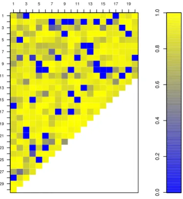
,
fork=1, . . . ,I−1 withsk =0.9(k−1). The entries of the first (second) rows determine the increase of the 183
cumulative claims of the first (second) triangle. Note that the structural connections among triangles, 184
i.e. the non-diagonal entries ofBk, decrease towards zero fork→I−1 to ensure that the cumulative 185
claims stabilize at a certain point in time. Furthermore, assume that the error termse∗1, . . . ,e∗nfrom the 186
representation in (8) are independently and normally distributed with mean zero and covarianceΣk. 187
The covariance matricesΣkare defined by multiplying the equicorrelation matrix with correlation 0.5 188
by the scalar 102s
kfork=1, . . . ,I−1. This choice ofΣkleads to error terms that become smaller for 189
k→I−1. If no shrinkage would be applied on the covariance matrices, then the error terms would 190
grow on average because they are linearly related to the cumulative claims of the previous period 191
which increase over time. Finally, the cumulative claimsC(m)i,k fori=1, . . . ,I,k=2, . . . ,Iandm=1, 2 192
can be computed according to the GMCL model in (1) by generating independent error terms from 193
the aforementioned error distribution. We have chosen the parametersAk,BkandΣksuch that the 194
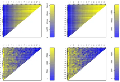
resulting run-off triangles resemble real data. The cumulative and incremental claims of two run-off 195
triangles simulated according to this data generating process are shown in Figure1. Note that the 196
patterns in these run-off triangles behave similar for every accident period. 197
Consider the prediction of a single cell E(Ci(m),k ) of subportfolio mfor i+k > I+1, i.e. the prediction of a future loss. Given historic claims ofMsubportfolios, the development parametersAk andBkof the GMCL model can be estimated fork=1, . . . ,I−1. Following the GMCL model these parameter estimators yield a corresponding prediction estimator ˆCi(m),k for E(Ci(m),k ). In order to measure the prediction accuracy of the estimator ˆCi(m),k , we consider itsmean squared error of prediction(MSEP), given by
MSEP(Cˆ(m)i,k ) =E(Cˆi(m),k −E(C(m)i,k ))2.
Since in general it is not possible to derive a simple expression for the MSEP, we adopt a Monte-Carlo simulation strategy to estimate this quantity. By repeatedly generatingMrun-off triangles as described before, fitting the GMCL model and predicting E(C(m)i,k )through the computation of the estimator ˆCi(m),k , we obtainJprediction estimators denoted by(Cˆi(m),k )1, . . . ,(Cˆ(m)i,k )J. Then, an estimator of the MSEP of
ˆ
C(m)i,k is given by
\
MSEP(Cˆi(m),k ) = 1
J J
∑
j=1((Cˆi(m),k )j−E(Ci(m),k ))2.
Smaller values of MSEP indicate a better prediction performance. In our simulation results we will 198
1 3 5 7 9 11 13 15 17 19 21 23 25 27 29
29 27 25 23 21 19 17 15 13 11 9 7 5 3 1
0
50000
100000
150000
200000
1 3 5 7 9 11 13 15 17 19 21 23 25 27 29
29 27 25 23 21 19 17 15 13 11 9 7 5 3 1
0
50000
100000
150000
1 3 5 7 9 11 13 15 17 19 21 23 25 27 29
29 27 25 23 21 19 17 15 13 11 9 7 5 3 1
0
5000
10000
15000
1 3 5 7 9 11 13 15 17 19 21 23 25 27 29
29 27 25 23 21 19 17 15 13 11 9 7 5 3 1
0
5000
10000
15000
Figure 1.Cumulative and incremental claims for a pair of dependent run-off triangles. The top figures show the cumulative claims of both triangles, whereas the bottom figures show the incremental claims. Development periods are on the horizontal axis, accident periods are on the vertical axis. The bar plot represents a color code indicating the magnitude of the numbers.
For data simulated as described before we consider three procedures: the SCL model in 200
combination with LS (in short SCL-LS) and the GMCL model in combination with FGLS and robust 201
MM-estimators (in short GMCL-FGLS and GMCL-MM respectively). As noted byZhang(2010, pp. 202
595-596) it is difficult to fit the SUR models for the upper right part of the triangles because the data 203
is scarce. To avoid numerical instabilities, it is recommended to use SCL for the development in the 204
tail. Naturally, we advice to combine the robust procedure based on MM-estimators with a robust SCL 205
method such as proposed inVerdonck and Debruyne(2011) for the tail development. Since the focus 206
of this paper is on the multivariate model, we present all results without the tail development part, i.e. 207
the final 10 development periods using traditional or robust SCL. 208
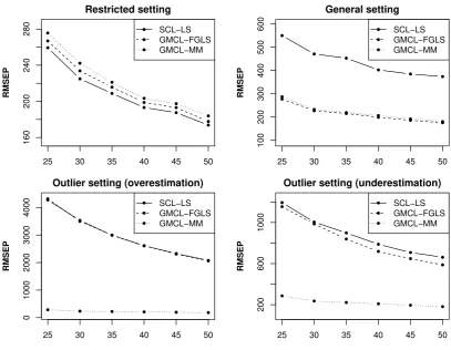
Consider the prediction of the expected claim size E(C(m)I,2 )form=1, 2. The top right panel of 209
Figure2shows the estimated RMSEP of ˆC(I1,2)for SCL-LS, GMCL-FGLS and GMCL-MM as a function 210
of the total number of accident periodsIranging from 25 to 50 forJ=1000 simulations. We can see 211
that the RMSEP estimates are larger for SCL-LS. This is expected because SCL does not take structural 212
connections among run-off triangles into account and contemporaneous correlations between the error 213
terms of the run-off triangles are ignored. Note that GMCL-FGLS and GMCL-MM perform similarly 214
in this setting where the triangles contain only regular measurements. Moreover, similar performance 215
was obtained for ˆC(I2,2)and hence, these results are omitted. 216
We now change the parameters Ak,Bk andΣk in the simulation design in such a way that it matches the SCL structure. Fork=1, . . . ,I−1 take
Ak = 0 0
!
, Bk = 1 0
0 1
!
25 30 35 40 45 50
160
200
240
280
Restricted setting
RMSEP
SCL−LS GMCL−FGLS GMCL−MM
25 30 35 40 45 50
100
200
300
400
500
600
General setting
RMSEP
SCL−LS GMCL−FGLS GMCL−MM
25 30 35 40 45 50
0
1000
2000
3000
4000
Outlier setting (overestimation)
RMSEP
SCL−LS GMCL−FGLS GMCL−MM
25 30 35 40 45 50
200
600
1000
Outlier setting (underestimation)
RMSEP
SCL−LS GMCL−FGLS GMCL−MM
Figure 2.RMSEP estimates of ˆC(I1,2)obtained from SCL-LS, GMCL-FGLS and GMCL-MM as a function ofIfor the restricted, general and outlier settings.
and letΣkbe the identity matrix multiplied with the scalar 102sk. In this setting SCL is optimal, whereas 217
the GMCL model uses too many parameters. Intercepts, slopes measuring the effects of the other 218
triangles and correlation parameters are unnecessary in this case. When we compare the results of 219
both estimation procedures, presented in the top left window of Figure2, we observe that the RMSEP 220
is only slightly larger for GMCL models. 221
To illustrate the sensitivity of the classical procedures and the robustness of MM-estimators, we 222
now consider the following outlier setting: for each pair of run-off triangles we replace the simulated 223
error terme2to generateC2,2with(105, 105)0. Based onJ=1000 generated pairs of triangles of this 224
kind, we obtained the results in the bottom left panel of Figure2. Clearly, both classical estimates break 225
down because they largely overestimate E(C(m)I,2 ), while the robust estimates are not influenced by 226
the outliers. The robust results are similar to the classical results that were obtained when no outliers 227
were present in the data. We also show the effect of small losses in run-off triangles. Therefore, we 228
consider a second outlier setting: for each pair of run-off triangles we replaceC2,2with(0, 0)0. The 229
bottom right plot of Figure2shows the RMSEP estimates for this outlier setting. Now, both classical 230
estimators underestimate E(C(m)I,2 )due to a small loss observed in accident period two, leading to large 231
RMSEP values. On the other hand, the robust method resists the effect of the outlier and still performs 232
well. In both outlier settings the robust method can also detect the outlier because the weight of the 233
corresponding accident period is zero as can be seen in Figure3for the first outlier setting. For the 234
second outlier setting the plot of weights is nearly identical. 235
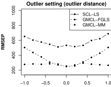
To illustrate the impact of the outlier’s distance to the regular data, we also consider a third outlier 236
Outlier setting (overestimation)
W
eights
1 4 7 10 13 16 19 22
0.0
0.2
0.4
0.6
0.8
1.0
Figure 3.Weights obtained from GMCL-MM for a pair of dependent run-off triangles with one outlier.
104(d,d)0wheredranges from -1 to 1. Non-contaminated error terms take values between -3000 and 238
3000 for the first development period. Therefore, the situations when|d|>0.3 are cases with outliers. 239
AgainJ=1000 bivariate run-off triangles are generated and the prediction accuracy of the expected 240
claim E(C(m)I,2 )is measured by MSEP. As opposed to the previous simulations we now fix the number 241
of accident periodsIto 25. Figure4contains the RMSEP results for different outlier distancesd. When
−1.0 −0.5 0.0 0.5 1.0
200
400
600
800
1000
Outlier setting (outlier distance)
RMSEP
SCL−LS GMCL−FGLS GMCL−MM
Figure 4.RMSEP estimates of ˆC(I1,2)obtained from SCL-LS, GMCL-FGLS and GMCL-MM as a function of the outlier distanced.
242
|d| ≤0.3 no outliers are generated and the prediction performance of the procedures GMCL-FGLS and 243
GMCL-MM are identical, as we have seen before. For situations with outliers the classical methods 244
yield large RMSEP values because their predictions under- or overestimate the target claim due to 245
the presence of the outliers. The larger the outlier distanced, the worse the prediction accuracy is for 246
non-robust methods. On the other hand, the prediction estimates obtained from the robust method 247
remain stable for all situations. 248
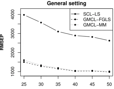
A more general case is to consider the prediction of E(C(m)I,k )form=1, 2 withk>2. In particular, 249
we considerk=15. We repeat the same procedure of squaringJ=500 pairs of dependent triangles 250
and measure the prediction accuracy of ˆC(m)I,15by means of RMSEP. The results for the general setting 251
are shown in Figure5. The performance of the different methods is comparable to their performance 252
in the previous setting when predicting E(C(m)I,2 ). However, sincek= 15 the prediction of E(C(m)I,15)
253
depends on 14 model fits, and consequently, the MSEP estimates of ˆC(m)I,15become much larger. The 254
prediction performance in the restricted setting and outlier settings (not shown) are also similar as 255
25 30 35 40 45 50
1000
2000
3000
4000
General setting
RMSEP
SCL−LS GMCL−FGLS GMCL−MM
Figure 5.RMSEP estimates of ˆC(I,151) obtained from SCL-LS, GMCL-FGLS and GMCL-MM as a function ofIfor the general setting.
We have also investigated how the position of the outlier influences the prediction performance. 257
Here the outlier’s position refers to the development period in which it has occurred because the effect 258
is similar for all accident years. If the outlier occurs after the target claim, then both the classical and 259
robust methods yield reliable prediction results for the target claim. However, when the outlier occurs 260
before the target claim, then the classical methods yield prediction estimates that are affected by the 261
outlier, while the robust method remains reliable. Only when the outlier appears in the upper right tail 262
of a run-off triangle, it will affect any method, whether it is robust or not, because there is not enough 263
data available in this tail to be able to identify an outlier. Since the position of outliers is unknown in 264
practice, this illustrates the importance of robust procedures which offer protection against outliers in 265
almost any position of the run-off triangles. 266
6. Real Data 267
To illustrate the new methodology, we consider an example with paid and incurred data from a motor 268
third party liability (MTPL) and a general third party liability (GTPL) insurance portfolio from a 269
non-life insurance company operating in Belgium. The data have been recorded between March 2008 270
and December 2015. Quarterly data are available leading to run-off triangles of dimension 31×31 271
shown in Figure6. Observe that from accident trimester 15 onwards the cumulative claim amounts 272
for MTPL become much smaller. This effect is due to a decrease in total premium volume, and hence, 273
also in total number of claims. For the GTPL data, accident trimester 1 seems suspicious. The claim 274
amounts are much larger in comparison to any other period. Finally, notice that for the first 15 accident 275
trimesters the losses in the subportfolios are almost fully developed, i.e. the changes in consecutive 276
cumulative claims are minuscule in the last development years. 277
We model these run-off triangles separately with SCL and jointly with GMCL. The joint model is 278
given by equation (1) with M = 3. The separate model simplifies the joint model by excluding 279
intercepts, structural connections and contemporaneous correlations. We have applied SCL-LS, 280
GMCL-FGLS and GMCL-MM to square the run-off triangles up until period 21. As explained before, 281
we exclude the tail development part in order to focus on the multivariate models. 282
TableA1in the Appendix contains the estimates of the development parameters and the sample 283
correlations between the resulting residuals obtained by SCL-LS for all development periods. While 284
the run-off triangles have been modeled separately, for some development periods there are substantial 285
correlations between the residuals which indicates that the independence assumption might be violated 286
for these data. 287
1 3 5 7 9 11 1315 17 1921 23 25 2729 31
31 29 27 25 23 21 19 17 15 13 11 9 7 5 3 1
0
5
10
15
20
25
1 3 5 7 9 11 13 15 1719 21 23 2527 29 31
31 29 27 25 23 21 19 17 15 13 11 9 7 5 3 1
0
10
20
30
40
1 3 5 7 9 11 1315 17 1921 23 25 2729 31
31 29 27 25 23 21 19 17 15 13 11 9 7 5 3 1
0
1
2
3
4
5
Figure 6.Cumulative run-off triangles (divided by 100000) of a real insurance portfolio. Top left: paid data of MTPL. Top right: incurred data of MTPL. Bottom left: paid data of GTPL. Development periods are on the horizontal axis, accident periods are on the vertical axis. The bar plot represents a color code indicating the magnitude of the numbers.
when predicting future losses in a triangle. From TableA2it can be seen that for some development periods these estimates are substantially different from zero. They improve the model fit and the prediction performance. The last three columns of TableA2contain the sample correlations between the residuals of the three run-off triangles, which have been obtained as
ˆ
ρmm0= σˆmm
0 √
ˆ
σmmσˆm0m0,
form,m0 =1, 2, 3, where ˆσmm0are the entries of the covariance matrix ˆΣk. Several moderate to large 288
correlations have been obtained which again supports the joint GMCL model for these data. 289
We now apply the robust method GMCL-MM which yields the development parameter estimates 290
shown in TableA3in the Appendix. Based on this robust procedure we can now detect possible 291
outliers. The weights assigned to each observation in the SUR models are shown in Figure7. The 292
smaller the weight, the more outlying is an observation with respect to the bulk of the data. For 293
example, from Figure7we can observe that in the first development period there are two major 294
outliers corresponding to accident trimesters 16 and 28 respectively. 295
The outliers identified by the GMCL-MM method may have affected the classical estimators, and 296
hence, also the prediction of future losses. Hence, in Table2we compare the total reserve estimates for 297
all methods. Let us first focus on the paid losses of the MTPL portfolio. The non-robust SCL-LS and 298
GMCL-FGLS methods both yield a total reserve estimate that is larger than for the robust GMCL-MM. 299
A close inspection of the predicted run-off triangles revealed that the transition from development 300
trimester 20 to 21 is highly responsible for these large differences. For development trimester 21 one 301
1 3 5 7 9 11 13 15 17 19
29 27 25 23 21 19 17 15 13 11 9 7 5 3 1
0.0
0.2
0.4
0.6
0.8
1.0
Figure 7.Weights obtained from GMCL-MM for a real insurance portfolio. Each row corresponds to an accident trimester used in the fitting procedure. Each columns represents a SUR model.
Table 2. Total reserve estimates for all run-off triangles of a real insurance portfolio obtained from SCL-LS, GMCL-FGLS and GMCL-MM.
Method Run-off Triangle
MTPL paid MTPL incurred GTPL paid
SCL-LS 1924001 -654695 386949
GMCL-FGLS 12198112 -1175336 -670116
GMCL-MM 167221 1043591 -128463
8. The SCL-LS and GMCL-FGLS fits for this transition period are both largely influenced by this 303
particular observation. Consequently, the predicted future losses from this development trimester 304
onward are much larger. On the other hand, the robust GMCL-MM method is much less influenced by 305
this observation and is able to flag this observation as an outlier. 306
Let us now consider the reserve estimates of the incurred losses. The two non-robust approaches 307
agree quite well. The difference is mainly caused by accident trimester 29 for which unexpectedly 308
small paid losses have been observed but at the same time large incurred losses were recorded. In 309
the joint GMCL model the development factorβ12for model 7 differs from zero and thus influences 310
the incurred losses obtained by GMCL-FGLS which is not the case for SCL-LS. Moreover, remark 311
that these reserve estimates are negative. Negative reserve estimates are often observed for incurred 312
run-off triangles due to overestimation of the losses. The robust total reserve estimate obtained by 313
GMCL-MM is much larger than for the non-robust methods. This indicates that the presence of outliers 314
has again affected the classical results. More specifically, in this case the classical procedures yield 315
smaller prediction estimates as compared to the robust procedure. For example, one can verify that for 316
the transition from development trimester 18 to 19 the prediction estimates obtained by GMCL-MM 317
are much larger than those obtained by GMCL-FGLS. 318
Finally, we also consider the estimated reserve for the GTPL portfolio. The unusual data in the 319
first accident trimester affect the total reserve estimates of both non-robust methods. On the other hand, 320
the robust GMCL-MM detected the deviating pattern in the first accident trimester as well as other 321
the available data. Note that the GMCL based methods yield negative reserve estimates for these data. 323
While negative reserve estimates are not uncommon for incurred losses, they are rather unusual for 324
run-off triangles with paid losses. However, the real data have been obtained from a small company 325
and the company informed us that for some claims there has been substantial recovery of initially paid 326
losses. These recoveries have an impact on the cumulative claims data which may explain the negative 327
reserve estimates in this case. 328
To further investigate the performance of the estimation methods, we now focus on the prediction 329
of the values on the last diagonal of all run-off triangles. To measure the accuracy of the predictions, 330
we consider their MSEP. More specifically, we leave out the last diagonal of all three run-off triangles, 331
apply the different methods on the remaining data and calculate the mean squared relative prediction 332
error for each method. The results are given in Table3for each subportfolio separately as well as all 333
portfolios jointly. While the three methods perform quite similar on the first two run-off triangles, this
Table 3.MSEP for the last diagonal of all run-off triangles (and totals) of a real insurance portfolio obtained from SCL-LS, GMCL-FGLS and GMCL-MM.
Method Run-off Triangle Total
MTPL paid MTPL incurred GTPL paid
SCL-LS 0.024 0.021 0.142 0.187
GMCL-FGLS 0.032 0.057 0.337 0.426
GMCL-MM 0.024 0.040 0.076 0.140
334
is not the case for the GTPL paid data as can be seen from Table3. The MSEP of GMCL-FGLS is large 335
for this run-off triangle. SCL-LS performs better, but not as good as GMCL-MM which is the only 336
method that yields reasonable performance for these data. As a result, GMCL-MM also shows the best 337
overall performance which illustrates that the outliers in these run-off triangles affect the predictions 338
of the non-robust methods. 339
7. Conclusion 340
In this paper we have presented a robust estimation method for the general multivariate chain 341
ladder model proposed byZhang(2010). Hence, our proposed methodology takes into account 342
contemporaneous correlations and structural connections between different run-off triangles and still 343
yields reliable results when the data are contaminated. Moreover, it allows us to automatically identify 344
the most influential and atypical claims in the run-off triangles. 345
It is important to further inspect the detected outliers and to understand the reasons for their 346
atypical behavior. If the outliers are errors or due to causes that are not likely to happen again in future, 347
then the robust results can be used as reserve estimates. However, if such atypical observations are 348
expected to re-occur in the future, it is necessary to model also their process (which is outside the 349
scope of this paper) and to predict how much extra reserve besides the robust total reserve estimate 350
is needed to cope with such atypical observations in future years. In such a case the final estimate 351
may for instance be equal to the robust total reserve estimate plus a safe margin when outliers lead to 352
an overestimation of the total reserve estimate. Note that it can also happen that outliers lead to an 353
underestimation of the total reserve estimate even if the atypical claims are larger than the expected 354
claims. 355
The robust GMCL method was applied on simulated run-off triangles illustrating its excellent 356
performance. From a portfolio analysis of real run-off triangles from a small non-life insurance 357
company in Belgium it was clear that the proposed robust methodology is helpful to gain insight in 358
the data and to build up a more realistic reserve, certainly when it is used in addition to the classical 359
Author Contributions:The authors contributed equally to this work. 361
Funding: This research was funded by International Funds KU Leuven grant numbers C16/15/068 and 362
C24/15/001, the CRoNoS COST Action grant number IC1408 and the Flemish Science Foundation (FWO) grant 363
number 1523915N. 364
Conflicts of Interest:“The authors declare no conflict of interest.” 365
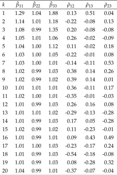
Appendix 366
Table A1.Development parameter estimates and empirical correlation estimates obtained from SCL-LS for a real insurance portfolio.
k βˆ11 βˆ22 βˆ33 ρ˜12 ρ˜13 ρ˜23
1 1.29 1.04 1.88 0.13 0.51 0.04 2 1.14 1.01 1.18 -0.22 -0.08 0.13 3 1.08 0.99 1.35 0.20 -0.08 -0.08 4 1.05 1.01 1.06 0.26 -0.02 -0.09 5 1.04 1.00 1.12 0.11 -0.02 0.18 6 1.03 1.00 1.05 -0.22 -0.01 0.08 7 1.03 1.00 1.01 -0.14 -0.11 0.53 8 1.02 0.99 1.03 0.38 0.14 0.26 9 1.02 0.99 1.02 0.39 0.14 0.01 10 1.01 1.01 1.01 0.36 -0.11 0.17 11 1.02 1.00 1.01 -0.35 -0.01 -0.03 12 1.01 0.99 1.03 0.26 0.16 0.08 13 1.01 1.01 1.02 -0.29 -0.13 -0.28 14 1.01 0.99 1.03 0.17 0.05 -0.28 15 1.02 0.99 1.02 0.11 -0.23 -0.01 16 1.01 0.99 1.01 0.09 0.43 0.49 17 1.01 1.00 1.03 -0.23 -0.17 0.24 18 1.01 0.99 1.03 -0.54 -0.18 -0.08 19 1.01 0.99 1.03 0.08 -0.28 0.32 20 1.04 0.99 1.01 -0.37 -0.07 -0.04
367
Ajne, B.. 1994. Additivity of chain-ladder projections. Astin Bulletin 24(2), 311–318. 368
Bilodeau, M. and P. Duchesne. 2000. Robust estimation of the SUR model. The Canadian Journal of Statistics 28(2), 369
277–288. doi:10.2307/3315978. 370
Braun, C.. 2004. The prediction error of the chain ladder method applied to correlated run-off triangles. Astin 371
Bulletin 34(2), 399–423. 372
Brazauskas, V.. 2009. Robust and efficient fitting of loss models: diagnostic tools and insights. North American 373
Actuarial Journal 13(3), 356–369. 374
Brazauskas, V., B. L. Jones, and R. Zitikis. 2009. Robust fitting of claim severity distributions and the method of 375
trimmed moments. Journal of Statistical Planning and Inference 139(6), 2028–2043. 376
Dreksler, S., C. Allen, A. Akoh-Arrey, J. A. Courchene, B. Junaid, J. Kirk, W. Lowe, S. O’Dea, J. Piper, M. Shah, 377
G. Shaw, D. Storman, S. Thaper, L. Thomas, M. Wheatley, and M. Wilson. 2015. Solvency II Technical Provisions 378
For General Insurers. British Actuarial Journal 20(1), 7–129. 379
England, P. D. and R. J. Verrall. 2002. Stochastic Claims Reserving in General Insurance. British Actuarial 380
Hubert, M., T. Verdonck, and O. Yorulmaz. 2017. Fast robust SUR with economical and actuarial applications. 382
Statistical Analysis and Data Mining 10(2), 77–88. doi:10.1002/sam.11313. 383
Koenker, R. and S. Portnoy. 1990. M-estimation of multivariate regressions. Journal of the American Statistical 384
Association 85(412), 1060–1068. doi:10.1080/01621459.1990.10474976. 385
Maronna, R. A., D. R. Martin, and V. J. Yohai. 2006.Robust Statistics: Theory and Methods. New York: John Wiley 386
and Sons. 387
Merz, M. and M. V. Wüthrich. 2007. Prediction error of the chain ladder reserving method applied to correlated 388
run-off triangles. Annals of Actuarial Science 2(1), 25–50. 389
Merz, M. and M. V. Wüthrich. 2008. Prediction error of the multivariate chain ladder reserving method. North 390
American Actuarial Journal 12(2), 175–197. 391
Nelder, J. A. and R. W. M. Wedderburn. 1972. Generalized Linear Models. Journal of the Royal Statistical Society. 392
Series A (General) 135(3), 370–384. 393
Peremans, K, P. Segaert, S. Van Aelst, and T. Verdonck. 2017. Robust bootstrap procedures for the chain-ladder 394
method. Scandinavian Actuarial Journal 2017(10), 870–897. doi:10.1080/03461238.2016.1263236. 395
Peremans, K. and S. Van Aelst. 2018. Robust Inference for Seemingly Unrelated Regression Models. Journal of 396
Multivariate Analysis to appear, arXiv:1801.04716. 397
Pitselis, G., V. Grigoriadou, and I. Badounas. 2015. Robust loss reserving in a log-linear model. Insurance: 398
Mathematics and Economics 64, 14–27. 399
Pröhl, C. and K. D. Schmidt. 2005. Multivariate chain-ladder. Dresdner Schriften zur Versicherungsmathematik. 400
Quarg, G. and T. Mack. 2004. Munich chain ladder.Blätter der DGVFM 26(4), 597–630. 401
Salibian-Barrera, M. and V. J. Yohai. 2006. A fast algorithm for S-regression estimates. Journal of Computational and 402
Graphical Statistics 15(2), 414–427. doi:10.1198/106186006X113629. 403
Schmidt, K. D.. 2006. Optimal and additive loss reserving for dependent lines of business. Casualty Actuarial 404
Society Forum, 319–351. 405
Verdonck, T. and M. Debruyne. 2011. The influence of individual claims on the chain-ladder estimates: Analysis 406
and diagnostic tool. Insurance: Mathematics and Economics 48(1), 85–98. 407
Verdonck, T. and M. Van Wouwe. 2011. Detection and correction of outliers in the bivariate chain–ladder method. 408
Insurance: Mathematics and Economics 49(2), 188–193. 409
Verdonck, T., M. Van Wouwe, and J. Dhaene. 2009. A robustification of the chain-ladder method.North American 410
Actuarial Journal 13(2), 280–298. 411
Wüthrich, M. V. and M. Merz. 2008. Stochastic claims reserving methods in insurance. John Wiley & Sons. 412
Zellner, A.. 1962. An Efficient Method of Estimating Seemingly Unrelated Regressions and Tests for Aggregation 413
Bias. Journal of the American Statistical Association 57(298), 348–368. doi:10.2307/2281644. 414
Zhang, Y.. 2010. A general multivariate chain ladder model. Insurance: Mathematics and Economics 46(3), 588–599. 415
k ˆβ01
ˆβ11 ˆβ21
ˆβ31
ˆβ02 ˆβ12
ˆβ22
ˆβ32 ˆβ03
ˆβ13
ˆβ23
ˆβ33
k ˆβ01 ˆβ11 ˆβ21
ˆβ31
ˆβ02
ˆβ12
ˆβ22 ˆβ32
ˆβ03 ˆβ13
ˆβ23
ˆβ33