University of South Carolina
Scholar Commons
Theses and Dissertations
2017
Improving Peptide Identification by Considering
Ordered Amino Acid Usage
Ahmed AL-Qurri
University of South Carolina
Follow this and additional works at:https://scholarcommons.sc.edu/etd
Part of theComputer Engineering Commons, and theComputer Sciences Commons
This Open Access Thesis is brought to you by Scholar Commons. It has been accepted for inclusion in Theses and Dissertations by an authorized administrator of Scholar Commons. For more information, please [email protected].
Recommended Citation
AL-Qurri, A.(2017).Improving Peptide Identification by Considering Ordered Amino Acid Usage.(Master's thesis). Retrieved from
IMPROVING PEPTIDE IDENTIFICATION BY CONSIDERING ORDERED AMINO ACID USAGE
by
Ahmed AL-Qurri
Bachelor of Science Sultan Qaboos University, 1998
Post-Graduate Diploma Sultan Qaboos University, 2016
Submitted in Partial Fulfillment of the Requirements
For the Degree of Master of Science in
Computer Science and Engineering
College of Engineering and Computing
University of South Carolina
2017
Accepted by:
John Rose, Director of Thesis
Jijun Tang, Reader
Gabriel A. Terejanu, Reader
ii
iii
ACKNOWLEDGEMENTS
I am using this opportunity to express my gratitude to everyone who supported
me throughout the course of this Master thesis. I am thankful for their aspiring guidance,
invaluably constructive criticism and friendly advice during the project work. I am
sincerely grateful to them for sharing their truthful and illuminating views on a number of
issues related to the project.
Mainly, I express my warm thanks to my thesis advisor Prof. John Rose for his
support and guidance. I would also like to thank Mr. Ryan Austin Systems Manager,
Computing Infrastructure for his support related to UNIX systems. Moreover, I would
like to thank Dr. Webb-Robertson from Pacific Northwest National Laboratory for
providing dataset for testing and also Dr. Craig Lawless from University of Manchester
iv
ABSTRACT
Proteomics has made major progress in recent years after the sequencing of the
genomes of a substantial number of organisms. A typical method for identifying peptides
uses a database of peptides identified using tandem mass spectrometry (MS/MS). The
profile of accurate mass and elution time (AMT) for peptides that need to be identified
will be compared with this database. Restricting the search to those peptides detectable
by MS will reduce processing time and more importantly increase accuracy. In addition,
there are significant impacts for clinical studies. Proteotypic peptides are those peptides
in a protein sequence that are most likely to be confidently observed by current MS-based
proteomics methods. There has been rapid improvement in the prediction of proteotypic
peptides for AMT studies based on amino acid properties such as amino acid content,
polarity, charge and hydrophobicity using a support vector machine (SVM) classification
approach. Our goal is to improve proteotypic peptide prediction. We describe the
development of a classifier that considers amino acid usage that has achieved a
classification sensitivity of 90% and specificity 81% on the Yersinia pestis proteome
(using 3-AAU). Using Ordered Amino Acid Usage (AAU) feature, we were able to
identify a different set of peptides that was not identified by the 35 peptides features that
STEP (Webb-Robertson, 2010)[2] have used. This means that Ordered Amino Acid
Usage (AAU) feature could complement other features used by STEP to improve
v
2010)[2] 35 amino acids features to complement Ordered Amino Acid Usage (AAU)
vi
TABLE OF CONTENTS
ACKNOWLEDGEMENTS ... iii
ABSTRACT ... iv
LIST OF TABLES ... viii
LIST OF FIGURES ... ix
LIST OF SYMBOLS ...x
LIST OF ABBREVIATIONS ... xi
CHAPTER 1:INTRODUCTION ...1
1.1PROBLEM AND HYPOTHESIS ...1
1.2IMPORTANCE OF TOPIC ...3
1.3BACKGROUND ...6
1.4RESEARCH METHODOLOGY ...8
1.5VERIFYING WEBB-ROBERTSON ET AL.RESULTS USING MATLAB MACHINE LEARNING BUILT IN FUNCTIONS ...9
CHAPTER 2:EVALUATIONUSINGAAU ...12
2.1EVALUATING AAU-BASED CLASSIFIERS ...12
2.2COMBINING THE 2-AAUFEATURES WITH STEPPFEATURE ...16
2.3FEATURE REDUCTION USING PCA ...19
CHAPTER 3:RESULTVERFICATION ...23
3.1VERIFICATION USING SECOND DATA SET ...23
vii
CHAPTER 4:FEATURESSELECTION ...26
4.1FEATURES SELECTION ...26
CHAPTER 5:DISCUSSIONOFRESULTS ...29
5.1ACCURACY FOR PROTEOTYPIC AND NON- PROTEOTYPIC PEPTIDE SEPARATELY ...29
5.2PREDICTION TIME ...31
5.3RECEIVER OPERATING CHARACTERISTIC (ROC)CURVE FOR DIFFERENT CONFIGURATION ...32
5.4LIMITATIONS AND KEY ASSUMPTIONS ...34
CHAPTER 6:CONCLUSION ...36
6.1CONTRIBUTIONS ...36
6.2SUMMERY ...36
viii
LIST OF TABLES
Table 1.1: Proteotypic peptide features STEPP ...4
Table 1.2: AUC values for within and across AMT dataset evaluation ...11
Table 1.3: Accuracy for different SVM kernels ...11
Table 2.1: Accuracy for 2 and 3 adjacent Amino Acids ...14
Table 2.2: Accuracy for 35 Features and 2-AAU feature combined ...16
Table 2.3: Accuracy for 35 Features and 3-AAU feature combined ...18
Table 3.1: Success Rate for Yeast dataset ...23
Table 4.1: Accuracy of 6 selected feature from STEPP and 2-AAU...27
Table 4.2: Accuracy of 6 selected feature from STEPP and 2-AAU...28
Table 5.1: Accuracy for proteotypic and non-proteotypic peptide separately using 2-AAU29 Table 5.2: Accuracy for proteotypic and non- proteotypic peptide separately using 3-AAU.. ...29
Table 5.3: Accuracy for proteotypic and non- proteotypic peptide separately using 7 selected feature and 2-AAU.. ...30
Table 5.4: Accuracy for proteotypic and non- proteotypic peptide separately using 7 selected feature and 3-AAU.. ...30
Table 5.5: Prediction Time using different configuration.. ...31
ix
LIST OF FIGURES
Figure 1.1: histogram for 8,073 identified Peptides probability ...10
Figure 1.2: Histogram for the 105,399 Peptides probability for unidentified peptides ...10
Figure 1.3: histogram for peptides score for identified ...10
Figure 1.4: peptides score for un-identified. ...10
Figure 1.5: Accuracy using different kernel types. ...11
Figure 2.1: Accuracy for 2 and 3 adjacent Amino Acids ...14
Figure 2.2 Venn diagram shows common classification (overlap area) and misclassification errors. ...15
Figure 2.3: Venn diagram shows common classification (overlap area) and misclassification errors. ...15
Figure 2.4: Accuracy for 35 Features and 2-AAU feature combined ...17
Figure 2.5: Comparing STEPP 35 feature with AAU+STEPP. AAU her is 2-AAU ...17
Figure 2.6: Accuracy for 35 Features and 3-AAU feature combined ...18
Figure 2.7: Comparing 3-AAU with 2-AAU ...19
Figure 2.8: Matlab ―explained‖ which shows the percentage of how each feature contributes to the variance of data. ...20
Figure 2.9: Errors calculated as a function of the number of included eigenvectors (components) for Linear kernel ...21
x
Figure 2.11: Errors calculated as a function of the number of included eigenvectors (components) for Polynomial kernel ...22
Figure 3.1: Accuracy for Yeast dataset with 2-AAU compared to one without AAU. ...24
Figure 3.2: Success rate for data-set combined using 2-AAU ...25
Figure 4.1: Accuracy for each feature of STEPP 35 features alone using LDA. This is used in feature selection to understand which feature has more weight (more important).26
Figure 4.2: Comparing accuracy of 6 selected feature from STEPP with 2-AAU and 3-AAU. ...28
Figure 5.1: Comparing accuracy for proteotypic and non- proteotypic peptide separately using different configuration...31
Figure 5.2: Comparing prediction Time using different configuration. ...32
xi
LIST OF ABBREVIATIONS
AAU ...Amino Acid usage
AUC ... Area under curve
LDA ... Linear Discriminant Analysis
MS ... Mass spectrometry
PCA ...Principal Component analysis
ROC ... Receiver operating characteristic
1
C
HAPTER1
INTRODUCTION
1.1 Problem and Hypothesis
Proteomics aim to identify and quantify all of the proteins present in a cell at a
specific moment. Such studies typically pose challenges owing to the high degree of
complexity of cellular proteomes and the low abundance of many of the proteins, which
necessitates highly sensitive analytical techniques. Mass spectrometry (MS) has
increasingly become the method of choice for analysis of complex protein samples.
MS-based proteomics is a discipline made possible by the availability of gene and genome
sequence databases and technical and conceptual advances in many areas, most notably
the discovery and development of protein ionization methods, as recognized by the 2002
Nobel prize in chemistry (2003) [15]. Although Mass spectrometry (MS) offers a
high-throughput approach to quantifying the proteome and therefore becomes the standard
method of proteomic analyses, however, a lot of computation is required to analyze those
large data STEP (Webb-Robertson, 2010)[2].
The first formulation of the peptides detectability problem was in 2006 (Tang,
2006) [1]. Since then, several algorithmic approaches have been proposed. Those
approaches use different machine learning techniques and all share common steps:
2
2) Use machine learning techniques on the training data to create a model for prediction.
Researchers have taken different approach to define the concept of prototypic
peptides. For example STEPP (Webb-Robertson, 2010) [2] defines prototypic peptides to
be those that have been included in the AMT database every time the parent protein is
observed. In contrast, PeptideSieve (Mallick, 2007) [3] and CONSeQuence (Eyers,
2011) [4] use peptides that have been observed in 50% of all identification of the
corresponding protein in a set of experiments. In this paper we used one of the three
training testing dataset used by STEPP (Webb-Robertson, 2010) [2] and adopt that
definition of prototypic peptides.
Researchers have used different features and different methods. For example
STEPP (Webb-Robertson, 2010) [2] uses 35 peptide features as input to the support
vector machine (SVM). PeptideSieve (Mallick, 2007) [3] uses 494 properties with
Gaussian mixture likelihood scoring function. Also, authors used different methods, for
example, ESPPredictor (Fusaro, 2009) [5] uses random Forests classification. While
others used neutral networks to classify peptides, such as Tang, et al. (Tang, 2006) [1].
In tandem MS experiments only a small number of peptides present can be
reliably identified. Presumably, those peptides that cannot be reliably detected do not
fragment appropriately for the spectrometer. We hypothesize that bonds between adjacent
amino acids are an important factor affecting how a peptide fragments. Consequently, we
propose to use an abstract model of bonds between adjacent amino acids as an additional
3
We refer to this feature as Ordered Amino Acid Usage (AAU). Specifically, we
implicitly model peptide bonds at an abstract level by looking at ordered adjacent amino
acids. To be clear, we do not explicitly model peptide bonds. Ordered amino acids tuples
capture the mutual information of these peptide fragments at an abstract level. We have
considered ordered adjacent amino acids (2-AAU) as well as ordered triples of adjacent
amino acids (3-AAU). In this research, we have used the 35 features that STEPP have
used, in addition to the new AAU feature.
1.2 Importance of topic
Several mass spectrometry-based quantitative proteomics methods attempt to
comprehensively identify and quantify constituent proteins in complex mixtures.
Differences in the abundance of proteins in distinct samples have enabled scientist to
Identify cellular functions and pathways affected by perturbations and disease.
Revealed new components and changes in the compositions of protein complexes
and organelles.
Enabled detection of putative disease biomarkers (Mallick, 2007) [6].
A standard method for identifying peptides uses databases of peptides identified
using tandem mass spectrometry (MS/MS). A unique advantage for identifying
proteotypic peptides for accurate mass and elution time (AMT) studies is that the
prediction of the detectable peptides along with accurate elution time prediction of these
peptides would allow for prediction via computer simulation of an AMT database
(database of peptides previously identified from tandem mass spectrometry [MS/MS]
4
MS/MS. As a result, accurate prediction of proteotypic peptides for these studies could
significantly reduce cost and time (Webb-Robertson, 2010) [2].
Different researchers have used different parameters and algorithms to calculate
predication of identified and unidentified peptides. For example, STEPP
Robertson, 2010) [2] used 35 features and used the SVM approach. STEPP
(Webb-Robertson, 2010) [2] achieved an accuracy measure of ~83% with SD of less than 0.038.
SD is calculated by first generating ROC curve.
STEPP (Webb-Robertson, 2010) [2] used the following proteotypic peptide features
shown on Table 1:
Table 1.1: Proteotypic peptide features STEPP (Webb-Robertson, 2010) [2]
Feature Index in STEPP Feature
1 Length
2 Molecular weight
3 Number of non-polar hydrophobic residues 4 Number of polar hydrophilic residues
5 Number of uncharged polar hydrophilic residues 6 Number of charged polar hydrophilic residues 7 Number of positively charged polar hydrophilic
residues
8 Number of negatively charged polar hydrophilic residues
9 Hydrophobicity—Eisenberg scale 10 Hydrophilicity—Hopp–Woods scale 11 Hydrophobicity—Kyte–Doolittle 12 Hydropathicity—Roseman scale 13 Polarity—Grantham scale 14 Polarity—Zimmerman scale 15 Bulkiness
5
(Receiver Operating Characteristic). The area under curve is a good overall
measurement of accuracy (AUC). That is the ability to correctly classify a peptide on
average. Hence, perfect classification method will have an AUC of one, while a random
classifier will have AUC of ~0.5.
AUC have been calculated for the 3 datasets, S.oneidensis, S.typhimurium and
Y.pestis. Moreover, for validation across organisms, each classifier is used on the other
datasets. For example, the SVM classifier generated from S.oneidensis is used to classify
the peptides for the remaining two organisms (Webb-Robertson, 2010) [2]. This result on
the AUC values shown on Table 2:
Table 1.2: AUC values for within and across AMT dataset evaluation (Webb-Robertson, 2010) [2]
Training organism Shewanella
oneidensis
Salmonella typhimurium
Yersinia pestis
Shewanella oneidensis 0.791 0.827 0.865
Salmonella typhimurium 0.773 0.841 0.857
Yersinia pestis 0.782 0.834 0.879
As stated earlier, the mean for AUC data on table 3 is 0.828 and SD is 0.038.
Our approach aims to complement the success achieved by this method by
introducing a new type of feature, Ordered Amino Acid Usage (AAU) that aim to
enhance the accuracy. Preliminary results indicate that Ordered Amino Acid Usage
6
1.3 Background
One of the first approaches to experimentally identify proteotypic peptides
associated with a specific MS technology was using an accurate mass and elution time
(AMT) strategy that employed high-resolution MS. This generated a set of peptides that
could be detected based on mass and elution time profile (Mallick , 2007) [6].
Using standard database search algorithms such as SEQUEST, a list of peptides
are identified. This list of peptides called potential mass tags (PMT) (Yates , 1998) [8].
The next stage is validation using high accuracy MS using both mass and elution time.
Once this achieved, future identification is done merely by selection of peptides from the
AMT database based on AMT measurement. This method is advantageous, particularly,
in complex samples such as plasma, because it offers great sensitivity and increased
throughput (May, 2007) [9].
Creating an AMT database for all organisms using experimentation is very challenging.
Tremendous work has been expended in cataloging peptides identified by MS/MS (Craig
, 2005) [10]. One example of such a database is the European Bioinformatics Institute
PRIDE database. Available: http://genesis.ugent.be/pride, PeptideAtlas, GPM, SBEAMS
and PRIDE (Mallick , 2007) [6].
Those databases are very beneficial for evaluating proteomes as they only need to
search a subset of potential peptides candidates (Kuster, 2005) [11]. However, populating
these databases for new organisms remains a challenge. To overcome those problems, it
proposed to use known properties associated with the high probability that a peptide will
7
hydrophobicity of the peptide (refer to Table 1). Using those properties, it is possible to
predict proteotypic peptides directly from a primary sequence. Success has been reported
using shotgun LC-MS/MS and gel-based MS proteomics (Kuster, 2005) [11] ( Mallick,
2007) [3] (Tang, 2006) [1].
Webb-Robertson et al. (2010), report an approach for the prediction of
proteotypic peptides for AMT studies based on simple sequence-derived properties using
a support vector machine (SVM) classification [2]. As discussed in the introduction, this
method has the advantage of simulating AMT databases without having to identity the
peptides via MS/MS.
Webb-Robertson et al (2010), use three databases collected for organisms Shewanella
oneidensis, Salmonella typhimurium and Yersinia pestis. They used a selection of 35
features (List of features on Table 1) for the prediction of proteotypic peptides for
LC-FTICR-MS.
Ermir Qeli et al. (2014), use a rank based algorithm called PeptideRank similar to
those used in information retrieval and web searches (Qeli, 2014) [12]. They use 574
different numerical peptide features. Examples of such features are 20 peptides relative
frequencies of each amino acid, 10 general peptides properties (length, mass, estimated
isoelectric point, etc.) and 5,444 averaged physicochemical properties that were extracted
from AAindex1 [14] (AAindex is a database of numerical indices representing various
physicochemical and biochemical properties of amino acids and pairs of amino acids)
8
1.4 Research Methodology
Preliminary results show that the performance of a classifier based only on the
3-AAU feature comparable to the performance of a classifier using peptides properties. An
SVM classifier trained using only the 3-AAU features achieve a sensitivity of 89.72%
and a specificity of 81.04%. If we compared this with result achieved by STEPP, STEPP
achieved average accuracy measure of ∼0.83 using 35 features (Webb-Robertson, 2010)
[12]. We integrated the AAU feature with a subset of the 35 features used in by
Webb-Robertson et al. in STEPP [12]. This resulted in an improved classification rate. We, also,
noticed that classification differences between AAU approach and the STEPP result in
the misclassification of different peptides subsets. This indicates that the some of the
features used in STEPP could complement the AAU feature. In addition, we achieved
comparable results by using a subset of features rather than all 35 features together with
AAU.
1.5 Verifying Webb-Robertson et al. Results using Matlab machine learning built in functions:
We started first by verification of the result that Webb-Robertson et al achieved
using the SVM. Webb-Robertson et al have calculated SVM using the linear SVM:
Where defines the separating hyper plane, z is the normalized data, and si is the i-th
support vector as defined by the training. We used Matlab built-in SVM functions such as
fitcsvm. We also used one of peptide training data sets published as Webb-Robertson et
9
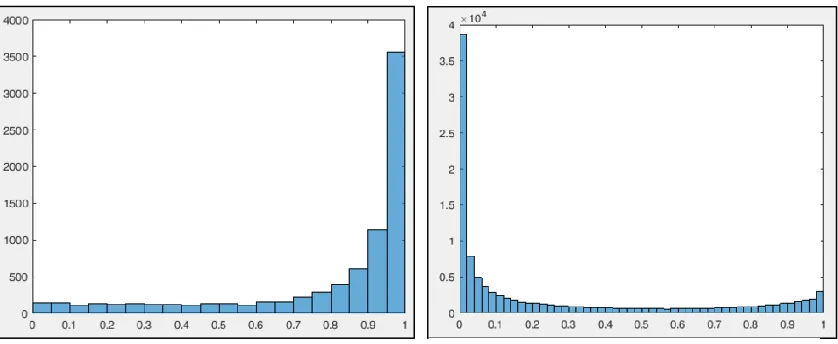
Diagrams in Figure 2 shows histogram for identified peptide probability, where
most of data are close to one. While Figure 3 shows histogram for un-identified peptide
with probability data close to zero.
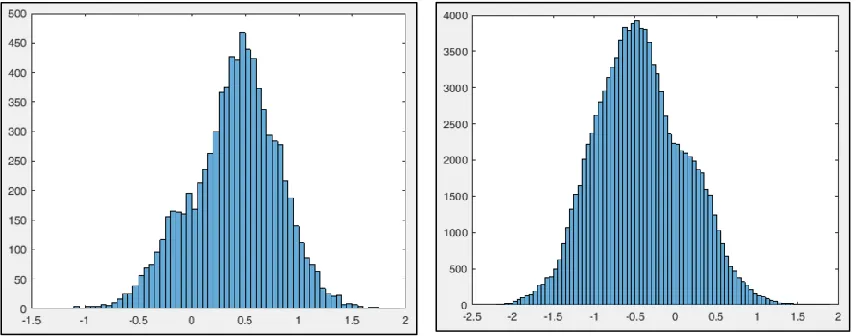
Similarly, Figure 4 below shows histogram for identified peptide score, which shows how far from the separating hyper plane.
Figure 1.1: histogram for 8,073 identified Peptides probability
10
Figure 1.4: peptides score for un-identified.
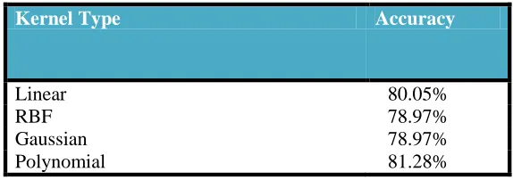
We evaluated different SVM kernels and noticed that while performance varies
between proteotypic and non-proteotypic peptides, the best average result is achieved
when the Polynomial kernel is used. For SVM result verification, we used 10-fold cross
validation and also calculated the confusion matrix. Accuracy is shown below for
different SVM kernels.
11
Table 1.3: Accuracy for different SVM kernels
Kernel Type Accuracy
Linear 80.05%
RBF 78.97%
Gaussian 78.97% Polynomial 81.28%
Below graph gives a visual representation for above table.
Figure 1.5: Accuracy using different kernel types.
77.50 78.00 78.50 79.00 79.50 80.00 80.50 81.00 81.50
Linear RBF Gaussian Polynomial
Accuracy
12
C
HAPTER2
EVALUATION USING AAU
2.1 Evaluating AAU-based Classifiers:
Next, we evaluated ordered adjacent amino acid tuples as a new feature. In order
to do that, we performed the following steps:
These steps are used to create separate log-probability matrices for proteotypic
peptides and non-proteotypic peptides. These matrices are later used to compute the
log-odds of a peptide being proteotypic. Notice, The log log-odds ratio is a common approach to
specifying a decision boundary in sequence classification.
1) We calculated the probability that two adjacent amino acids appear in proteotypic
and nonproteotypic peptide. This result in two matrices, one for proteotypic
peptide and another for nonproteotypic peptide. Each matrix column and row
represents a letter that correspond to an amino acid. So for example, columns of
matrix are labeled from A… Z and also for rows. Each element of the matrix
represents a bond between adjacent amino acids. In the case of these AAU
models, overlapping pairs were extracted from the coding sections of genomes. If
<a1a2a3…an> is a contiguous sequence of n amino acids, there are n – 1 pairs in
13
2) occurrences of each of the 400 (202) possible ordered pairs for a genome was
tabulated. The histogram is then normalized to sum to 1.
3) In order to avoid underflow when multiplying, a natural log is taken for each
element.
4) Since there are possibly elements with values equal to zero, epsilon is added to all
elements to mitigate the issue of taking log of zero.
The following steps were used to calculate log odds of peptide being proteotypic:
5) Assuming we have a new peptide ―EGALVQK‖. We look up the log odds values
of the adjacent amino acids ―EG‖, ―GA‖, ―AL‖,‖LV‖, ―VQ‖, ‖QK‖ in the two
log-probability matrices we created above ,using for example ―E‖ as a row index
and ―G‖ as a column index.
6) We sum up the log-probabilities from above step for each 2 adjacent amino acid,
so for ―EGALVQK‖, we sum up probabilities for ―EG‖, ―GA‖, ―AL‖,‖LV‖,
―VQ‖ and ‖QK‖. Again, we do this twice, once for the proteotypic peptide matric
and also for the non-proteotypic peptide model.
7) We derive the log odd ratio by divide the proteotypic log-probability by the non-
proteotypic log-probability. If the result is less than one, it’s classified as a
proteotypic peptide, otherwise non-proteotypic.
The process described above also repeated for three adjacent amino acids, i.e.
14
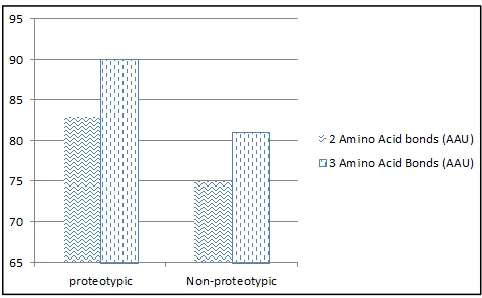
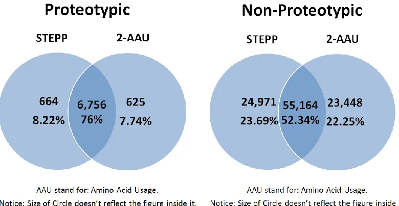
The best result was achieved using 3-AAU model. For the 2-AAU model, the sensitivity
was 83% and the specificity was 74.59%. In the case of the 3-AAU model, the sensitivity
was 89.72% and the specificity was 81.04%. The figure below summarizes this result.
Table 2.1: Accuracy for 2 and 3 adjacent Amino Acids
Proteotypic Non-proteotypic
2 Amino Acid bonds (AAU) 83% 75% 3 Amino Acid Bonds (AAU) 90% 81%
Below diagram (Figure 2.1) gives visual representation for same result.
Figure 2.1: Accuracy for 2 and 3 adjacent Amino Acids
This result suggests that the 2-AAU or 3-AAU feature could be combined with a
subset of the 35 features used by STEPP to achieve even better accuracy. We
demonstrate this in section 5.
As a preliminary step, we created a Venn diagram to depict the classification results of
STEPP and our simple 2-AAU-based classifier. In the case of proteotypic peptides, both
15
additional 8% of actual proteotypic peptides. This Venn diagram is shown below in
Figure 8 for proteotypic peptides and Figure 9 for nonproteotypic peptides. In figure 8,
we see that STEPP and the simple 2-AAU-based classifier disagree on a significantly
larger ~23% of actual nonproteotypic peptides. Notice, the shaded region in figure 8 is
where STEPP and AAU methods agree that this peptide is proteotypic. Likewise, the
shaded region in figure 9 is where STEPP and AAU methods agree that this peptide is
nonproteotypic.
2.2 Combining the 2-AAU Features with STEPP Feature:
The next stage is to combine the Ordered Amino Acid Usage (AAU) (2-AA)
feature with an appropriate subset of the 35 STEPP features to increase the accuracy of
peptide identification. We expected this to be possible since the two methods miss-Figure 2.2: Venn diagram shows common
classification (overlap area) and misclassification errors.
Figure 2.3: Venn diagram shows common classification (overlap area) and
16
classify peptides differently. Hence, there is room for improvement as the feature sets
possibly complement each other. The first approach was to simply add the Ordered
Amino Acid Usage (AAU) feature to the set of STEPP features by adding one new
column that represents the new AAU feature to the matrix that contains the 35 feature
used in STEPP (Webb-Robertson et al.). The new column is created by calculating log
odds values for each peptide.
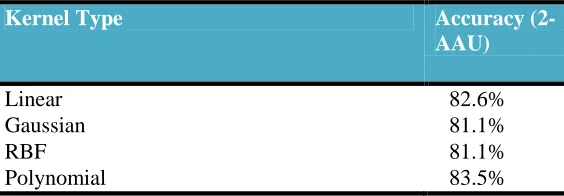
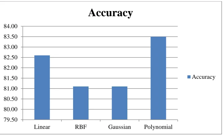
Table 5 below shows the improved accuracy after combing the two methods (AAU and
STEPP).
Table 2.2: Accuracy for 35 Features and 2-AAU feature combined
Kernel Type Accuracy
(2-AAU)
Linear 82.6%
Gaussian 81.1%
RBF 81.1%
Polynomial 83.5%
17
Figure 2.4: Accuracy for 35 Features and 2-AAU feature combined
Comparing the result (Table 5) that with previous result that uses STEPP 35
features only (Table 3), indicate there is some improvement. Below Figure (11) compare
the two methods. In the next section we describe a subset of features that achieve similar
results as that achieved by using all of these features.
Figure 2.5: Comparing STEPP 35 feature with AAU+STEPP. AAU her is 2-AAU
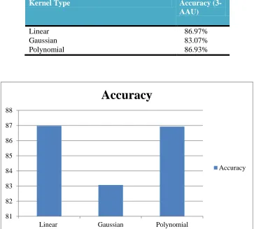
Likewise, we repeated the test using 3-AAU, ( 3 adjacent amino acid). 3-AAU gave a
much better result:
79.50 80.00 80.50 81.00 81.50 82.00 82.50 83.00 83.50 84.00
Linear RBF Gaussian Polynomial
Accuracy
18
Table 2.3: Accuracy for 35 Features and 3-AAU feature combined
Kernel Type Accuracy
(3-AAU)
Linear 86.97%
Gaussian 83.07%
Polynomial 86.93%
Figure 2.6: Accuracy for 35 Features and 3-AAU feature combined
Notice, unlike 2-AAU, liner kernel gave the best performance. In order to compare the
performance for 3-AAU with 2-AAU
81 82 83 84 85 86 87 88
Linear Gaussian Polynomial
Accuracy
19
Figure 2.7: Comparing 3-AAU with 2-AAU
Notice by looking at above figure with compare 3-AAU to 2-AUU. There is a major
improvement. For example, there is more than 4% improvement in linear kernel.
2.3 Feature Reduction using PCA:
We tried to use Principle Component Analysis (PCA) to give us insight to see
which feature of the STEPP 35 feature has more contribution. However, eventually, we
have used instead LDA. Nevertheless, for sake of completeness, I’m explaining here the
analysis I have done using PCA.
Principle Component Analysis (PCA) for the 35 features has been calculated. The aim is
to see if some of the features are dependent on each other and hence eliminate redundant
78 79 80 81 82 83 84 85 86 87 88
Linear Gaussian Polynomial
Comparing 3-AAU with 2-AAU
3-AAU
20
features. The advantage of feature elimination is that, by reducing the numbers of
unnecessary features, the SVM performance may be improved.
When calculating Principle Components, Matlab outputs a variable called
―explained‖ which shows the percentage of how each feature ―explains‖ the variance of
the data. The chart of the values of the ―explained‖ vector is shown below:
Figure 2.8: Matlab ―explained‖ which shows the percentage of how each feature contributes to the variance of data.
In addition, the empirical and uniform classification error is calculated as a function of
the number of included eigenvectors (components). This step is repeated using Linear,
Gaussian, and Polynomial kernel types. The graphs for each have been plotted below:
0 5 10 15 20 25 30 35
1 3 5 7 9 11 13 15 17 19 21 23 25 27 29 31 33 35
Explained value for Each Dimension
21
Figure 2.9: Errors calculated as a function of the number of included eigenvectors (components) for Linear kernel
Figure 2.10: Errors calculated as a function of the number of included eigenvectors (components) for Gaussian kernel
0 0.1 0.2 0.3 0.4 0.5 0.6
1 3 5 7 9 11 13 15 17 19 21 23 25 27 29 31 33 35
Linear
Uniform Error
0 0.1 0.2 0.3 0.4 0.5
1 3 5 7 9 11 13 15 17 19 21 23 25 27 29 31 33 35
Gaussian (RBF)
22
Figure 2.11: Errors calculated as a function of the number of included eigenvectors (components) for Polynomial kernel
0 0.2 0.4 0.6
1 3 5 7 9 11 13 15 17 19 21 23 25 27 29 31 33 35
Polynomial
23
CHAPTER
3
RESULT VERFICATION
3.1 Verification Using Second Data Set:
Our initial work used the Yersinia pestis data set that was also used for STEPP
(Webb-Robertson) [12]. We identified a second proteotypic peptide data set from a paper
titled “CONSeQuence: Prediction of Reference Peptides for Absolute Quantitative
Proteomics Using Consensus Machine Learning Approaches” [3]. The data set is for
Saccharomyces cerevisiae. The data is spilt on 2/3 for training and 1/3 for verification.
The results are shown the figure below.
Table 3.1: Success Rate for Yeast dataset
Proteotypic Non-proteotypic
24
Figure 3.1: Accuracy for Yeast dataset with 2-AAU compared to one without AAU.
3.2 Testing the two data sets combined:
25
Figure 3.2: Success rate for data-set combined using 2-AAU
70 72 74 76 78 80 82 84 86 88 90
proteotypic nonproteotypic
Success rate for data-set combined
26
CHAPTER
4
FEATURE SELECTION
4.1 Features Selection
One of the objectives of this research is to select a subset of the features used by STEPP to both improve accuracy and reduce computation time. We have used Linear Discriminant Analysis (LDA) to test and see which features contributing more. It is computationally not possible to exhaustively examine all possible combinations of features. Instead we examined each feature individually using LDA by looking at LDA loadings (Figure 19).
Figure 4.1: Accuracy for each feature of STEPP 35 features alone using LDA. This is used in feature selection to understand which feature has more weight (more important).
0 10 20 30 40 50 60 70 80 90 100
7 17 1 9 3 5 31 24 20 11 25 32 29 18 33 10 15 28 Accuracy
Using Linear Discriminant Analysis
(LDA) for Feature Selection
27
We noticed that it’s possible to achieve 82% accuracy using 7 features only. These features are:
Ordered Amino Acid Usage
Number of positively charged polar hydrophilic residues
Amino acid singlet counts: Proline (P)
Length
Number of non-polar hydrophobic residues
Number of polar hydrophilic residues
Number of charged polar hydrophilic residues
Notice that the features in Figure 6 are ordered based on their individual LDA score. We plan on looking at a more sophisticated approach to feature selection to either improve this result or confirm that this is optimal subset of the 35 STEPP features to use in conjunction with ordered amino acid usage.
In order to see how the how the new selected feature will perform, tests have been repeated with this feature subset only.
Table 4.1: Accuracy of 6 selected feature from STEPP and 2-AAU.
Kernel Type Accuracy
(2-AAU)
Linear 82.59%
Gaussian 81.07%
Polynomial 81.07%
28
Table 4.2: Accuracy of 6 selected feature from STEPP and 2-AAU.
Kernel Type Accuracy
(3-AAU)
Linear 86.45%
Gaussian 82.90%
Polynomial 59.47%
Below chars compares the 2 tables above:
Figure 4.2: Comparing accuracy of 6 selected feature from STEPP with 2-AAU and 3-AAU.
0% 10% 20% 30% 40% 50% 60% 70% 80% 90% 100%
Linear Gaussian Polynomial
Accuracy for 2 & 3 AAU using selected
features
Accuracy (2-AAU)
29
CHAPTER
5
DISCUSSION OF RESULTS
5.1 Accuracy for proteotypic and non- proteotypic peptide separately:
The above accuracy are based on 10-fold cross-validation error (―crossval‖ in Matlab). However, you might want to see how many proteotypic peptide have been classified correctly and visa-versa. Below table list accuracy for proteotypic and non-proteotypic peptide separately. The table below show the case for STEPP 35 feature with 2-AUU:
Table 5.1: Accuracy for proteotypic and non- proteotypic peptide separately using 2-AAU.
Kernel Type Accuracy (2-AAU) proteotypic Accuracy (2-AAU)
non-proteotypic
1 Linear 87.99% 77.190% 2 Gaussian 97.51% 87.257% 3 Polynomial 18.75% 76.81%
30
Table 5.2: Accuracy for proteotypic and non- proteotypic peptide separately using 3-AAU.
Kernel Type Accuracy (3-AAU)
proteotypic
Accuracy (3-AAU) non-proteotypic
4 Linear 95.11% 78.89% 5 Gaussian 87.61% 87.68% 6 Polynomial 96.96% 85.53%
The last case is for the 7 selected features:
Table 5.3: Accuracy for proteotypic and non- proteotypic peptide separately using 7 selected feature and 2-AAU.
Kernel Type Accuracy (2-AAU with
selected feature) proteotypic
Accuracy (2-AAU with selected feature) non-proteotypic
7 Linear 89.26% 74.95% 8 Gaussian 95.57% 83.26% 9 Polynomial 18.75% 76.81%
Table 5.4:Accuracy for proteotypic and non- proteotypic peptide separately using 7 selected feature and 3-AAU.
Kernel Type Accuracy (3-AAU with selected feature) proteotypic
Accuracy (3-AAU with selected feature) non-proteotypic
10 Linear 94.75% 78.185% 11 Gaussian 97.14% 83.90% 12 Polynomial 18.09% 92.19%
31
Figure 5.1: Comparing accuracy for proteotypic and non- proteotypic peptide separately using different configuration.
Notice, since this method, unlike the previous one, don’t use 10-fold validation, it might be prone to over fitting.
5.2 Prediction Time:
To get an understanding of how long predication time takes for each configuration, we have recorded the required time to predict if a peptide is proteotypic or non- proteotypic (call to predict function). Below table list time of each configuration:
0% 20% 40% 60% 80% 100%
1 2 3 4 5 6 7 8 9 10 11 12
Accuracy for proteotypic and non-
proteotypic peptide separately for
different configuration
Accuracy for proteotypic
32 Table 5.5: Prediction Time using different configuration.
configuration Time in seconds to
predict 8,073 peptide
1 Linear (STEPP 35 feature and 2-AUU combined) 6.918 2 Linear (STEPP 35 feature and 3-AUU combined) 3.675 3 Gaussian (STEPP 35 feature and 2-AUU combined) 13..142 4 Gaussian (STEPP 35 feature and 3-AUU combined) 8.250 5 Polynomial (STEPP 35 feature and 2-AUU combined) 12.783 6 Polynomial (STEPP 35 feature and 3-AUU combined) 2.417 7 Linear (STEPP 7 selected feature and 2-AUU combined) 2.521 8 Linear (STEPP 7 selected feature and 3-AUU combined) 1.862 9 Gaussian (STEPP 7 selected feature and 2-AUU combined) 10.287 10 Gaussian (STEPP 7 selected feature and 3-AUU combined) 14.454 11 Polynomial (STEPP 7 selected feature and 2-AUU combined) 2.565 12 Polynomial (STEPP 7 selected feature and 3-AUU combined) 1.967
Figure 5.2: Comparing prediction Time using different configuration.
Notice the fastest prediction time happened when linear kernel with selected feature from STEPP and 3-AAU combined.
5.3 Receiver Operating Characteristic (ROC) Curve for different Configuration: 0 5 10 15 20
1 2 3 4 5 6 7 8 9 10 11 12
Prediction Time in Seconds for 8,073
peptide for each configuration
33
Receiver Operating Characteristic (ROC) curves for different configurations have been generated and area under the curve (AUC) values have been calculated.
Below ROC curve shows ROC with different Configuration.
34 Table 5.6: AUC values for different configuration.
Configuration AU
C
1 Gaussian (STEPP 35 feature and 3-AUU combined) 0.98 2 Gaussian (STEPP 35 feature and 2-AUU combined) 0.97 3 Polynomial (STEPP 35 feature and 3-AUU combined) 0.96 4 Gaussian (STEPP 7 selected feature and 3-AUU combined) 0.95 5 Polynomial (STEPP 35 feature and 2-AUU combined) 0.94 6 Gaussian (STEPP 7 selected feature and 2-AUU combined) 0.94 7 Linear (STEPP 35 feature and 3-AUU combined) 0.93 8 Linear (STEPP 7 selected feature and 3-AUU combined) 0.92 9 Linear (STEPP 35 feature and 2-AUU combined) 0.88 10 Linear (STEPP 7 selected feature and 2-AUU combined) 0.87 11 Polynomial (STEPP 7 selected feature and 3-AUU combined) 0.83 12 Polynomial (STEPP 7 selected feature and 2-AUU combined) 0.60
5.4 Limitations and key Assumptions
There are three factors to govern the likelihood of observing a peptide in a
proteomics experiment: One, the chemical properties of the peptides and its parent
protein. Two, the limitation of the peptides identification protocol, including the
pre-processing of the sample, the MS instruments and software tools used for mass spectrum
analysis. And three, the abundance of the peptides in the sample that compete with this
peptides in the identification procedure (Tang, 2006) [1].
We used the same definition of proteotypic peptide that Webb-Robertson et have
used. Proteotypic peptides are those that have been included in the ATM database at any
time that the parent protein is observed, rather than requiring minimal observations of
35
The selection of peptides training set is a very crucial step in machine learning. For the
binary peptide detectability predication problem, both observed and non-observed
peptides should be represented in the training set to avoid bias and over-fitting in the later
learning process. Ideally there should be no bias against specific protein classes (Qeli, 2014) [12].
In our analysis we used peptides that have been provided by Webb-Robertson et
36
CHAPTER
6
CONCLUSION
6.1 Contributions
The aim of this thesis is to help improve the accuracy of peptides identification
and classification which have been gaining momentum due to their ability to generate
accurate quantitative data that is mostly relevant to system biology studies and clinical
use.
This thesis will explore bonds between amino acids as a new identification
feature. As mentioned previously, this new feature will be used to complement the
existing 35 features used by Webb-Robertson et al. and reduce the unnecessary features
in order to optimize Support Vector Machine (SVM) performance.
6.2 Summery
The most important conclusion of this research is that, the use of AAU feature
representing bonds between adjacent amino acids improves proteotypic peptide
prediction. The 3-AAU model is superior to the 2-AAU model. In addition, we used LDA
to select a subset of six of the STEPP features. Together with the AAU feature, a
classifier based on these features achieves classification accuracy similar to that achieved
37
A paper has been published based on this thesis. Citing of the paper is:
Ahmed Al-qurri and John Rose. "Improving Peptide Identification By Considering
Ordered Amino Acid Usage." Bioinformatics and Computational Biology (2017):
38
REFERENCES
[1] Tang, Haixu, et al. "A computational approach toward label-free protein
quantification using predicted peptide detectability." Bioinformatics 22.14 (2006): e481-e488.
[2] Webb-Robertson, Bobbie-Jo M., et al. "A support vector machine model for the prediction of proteotypic peptides for accurate mass and time proteomics."
Bioinformatics 24.13 (2008): 1503-1509.
[3] Mallick, Parag, et al. "Computational prediction of proteotypic peptides for quantitative proteomics." Nature biotechnology 25.1 (2007): 125-131.
[4] Eyers, Claire E., et al. "CONSeQuence: prediction of reference peptides for absolute quantitative proteomics using consensus machine learning approaches." Molecular & Cellular Proteomics 10.11 (2011): M110-003384.
[5] Fusaro, Vincent A., et al. "Prediction of high-responding peptides for targeted protein assays by mass spectrometry." Nature biotechnology 27.2 (2009): 190-198.
[7] Smith, Richard D., et al. "Review: The Use of Accurate Mass Tags for High-Throughput Microbial Proteomics." Omics: a journal of integrative biology 6.1 (2002): 61-90.
[8] Yates, John R., et al. "Method to compare collision-induced dissociation spectra of peptides: potential for library searching and subtractive analysis." Analytical chemistry 70.17 (1998): 3557-3565.
[9] May, Damon, et al. "A platform for accurate mass and time analyses of mass spectrometry data." Journal of proteome research 6.7 (2007): 2685-2694.
[10] Craig, Robertson, John P. Cortens, and Ronald C. Beavis. "The use of proteotypic peptide libraries for protein identification." Rapid communications in mass spectrometry 19.13 (2005): 1844-1850.
39
[12] Qeli, Ermir, et al. "Improved prediction of peptide detectability for targeted proteomics using a rank-based algorithm and organism-specific data." Journal of proteomics 108 (2014): 269-283.
[13] Tang, Haixu, et al. "A computational approach toward label-free protein
quantification using predicted peptide detectability." Bioinformatics 22.14 (2006): e481-e488.
[14] Kawashima, Shuichi, et al. "AAindex: amino acid index database, progress report 2008." Nucleic acids research 36.suppl 1 (2008): D202-D205.
![Table 1.1: Proteotypic peptide features STEPP (Webb-Robertson, 2010) [2]](https://thumb-us.123doks.com/thumbv2/123dok_us/8372866.1384130/16.612.123.490.399.676/table-proteotypic-peptide-features-stepp-webb-robertson.webp)
![Table 1.2: AUC values for within and across AMT dataset evaluation (Webb-Robertson, 2010) [2]](https://thumb-us.123doks.com/thumbv2/123dok_us/8372866.1384130/17.612.84.529.401.468/table-auc-values-amt-dataset-evaluation-webb-robertson.webp)