University of South Carolina
Scholar Commons
Theses and Dissertations
2017
Non-Destructive Evaluation Of Composites:
Predictive Ultrasonic Guided-Waves Modeling,
Non-Destructive Material Characterization, And
The Application To Aerospace Structures
Darun Barazanchy
University of South Carolina
Follow this and additional works at:https://scholarcommons.sc.edu/etd
Part of theMechanical Engineering Commons
This Open Access Dissertation is brought to you by Scholar Commons. It has been accepted for inclusion in Theses and Dissertations by an authorized administrator of Scholar Commons. For more information, please [email protected].
Recommended Citation
Barazanchy, D.(2017).Non-Destructive Evaluation Of Composites: Predictive Ultrasonic Guided-Waves Modeling, Non-Destructive
Material Characterization, And The Application To Aerospace Structures.(Doctoral dissertation). Retrieved from
NON-DESTRUCTIVE EVALUATION OF COMPOSITES
PREDICTIVE ULTRASONIC GUIDED-WAVES MODELING, NON-DESTRUCTIVE MATERIAL CHARACTERIZATION, AND THE APPLICATION TO AEROSPACE STRUCTURES
by
Darun Barazanchy
Bachelor of Science
Delft University of Technology, 2011
Master of Science
Delft University of Technology, 2013
Submitted in Partial Fulfillment of the Requirements
for the Degree of Doctor of Philosophy in
Mechanical Engineering
College of Engineering and Computing
University of South Carolina
2017
Accepted by:
V. Giurgiutiu, Major Professor
M. van Tooren, Committee Member
P. Ziehl, Committee Member
L. Yu, Committee Member
B. Lin, Committee Member
A
CKNOWLEDGMENTS
“If I have seen further, it is by standing on the shoulders of giants"
-Sir. Isaac Newton
The words expressed by Sir. Isaac Newton cannot be more true and are valid in both my
academic and personal life. Words cannot describe my gratitude to those who have helped
along the way, yet I will try. My special thanks to
• Dr. G; My academic supervisor who asked the right and challenging questions, who
kept me on track and his unending support and patience;
• Dr. van Tooren, Dr. Ziehl, Dr. Yu, Dr. Lin; For being part of my committee, reading
my work, questioning and providing feedback given such that this document was up
to standards;
• Dr. Martinez, Dr. Rocha; For the guidance, support, advice and sharing your
knowledge while I was at the National Research Council Canada, at TU Delft and
afterwards.
• Dr. Poddar, Dr. Roth, Erik, Hanfei and all the other LAMSS colleagues; For the
countless interesting discussions, ideas, feedback and suggestions. To Banibrata and
William, I won’t to forget our tea and coffee breaks;
• Wout, Arturs, Roudy and all the other McNair colleagues; For the great discussions
we all had during lunch in which the world’s problems were debated and solved at
• Jan Hol, Gillian, Sonell, Noud, Eric, Daniel, Fardin; For helping to fatigue test the
wall at the coffee machine and sharing your knowledge;
• Wessel, Stephen, Guillermo, Sean, Alex, Jack; Friends like you made Columbia
bearable!
• Gabriel, Ruben, Rijk, Koen, Jan, Julius en de dames Esma, Emel en Elise – Coon and
Friends groep; Waar zal ik beginnen? Al het bovenstaande en nog meer is geldig voor
jullie allen. Dank!;
• Heleen (molz) en Bas (schoonheid); Voor jullie steun en liefde door de jaren heen!
• Marten, Tom en Lucas; Mijn Nederlandse broers, voor al de mooie momenten die we
hadden en die nog gaan komen.
• Mijn moeder Suad en broer Lauk; Zonder jullie was dit nooit mogelijk en dat zal ik
nooit vergeten.
for it were your shoulders which made me see further.
This research was partially supported by: (i) Skolkovo Institute of Science and
Technology, Russia; (ii) Fokker GKN Aerospace; and (iii) National Aeronautics and Space
A
BSTRACT
To predict guided wave dispersion curves, it is common to use different solution
approaches depending on the material type (isotropic or anisotropic) of the medium in
which the wave propagates. The two different solution methods are defined in different
domains, frequency-phase velocity domain for isotropic materials and wavenumber-phase
velocity domain for anisotropic materials. This may lead to difficulties and unsatisfying
results when predicting the dispersion curves for hybrid laminates which contain
both isotropic and anisotropic materials. Therefore, a unified formulation defined in
the wavenumber-phase velocity domain to accomodate both isotropic and anisotropic
materials, as well as hybrid combinations, is desired. The unified analytic method (UAM)
proposed in this dissertation is a simple and mathematically straightforward formulation
that utilizes Christoffel’s equation for a lamina to obtain the eigenvalues and eigenvectors.
The eigenvalues and eigenvectors are used to set up the field matrix from which the
dispersion curves could be retrieved using a newly developed approach called the phase
approach. As last, the dispersion curves are grouped and sorted using a modeshape
analysis.
It is important to realize that predictions depend on the accuracy of the stiffness matrix
input for the UAM. Common practice is to determine the required material properties
using destructive mechanical testing procedures in combination with assumption based
on the material type. However, when the predicted dispersion curves varied significantly
from those obtained experimentally, the source of error was identified as the accuracy of
the stiffness matrix. A new non-destructive characterization method that combines the
LAMSS ultrasonic immersion technique is demonstrated to retrieve the stiffness matrix for
a unidirectional and woven fabric composite.
The retrieved stiffness matrix using the LAMSS ultrasonic immersion technique was
compared to the stiffness matrix reported in the literature. In the case of the woven fabric,
in-house mechanical testing was performed as well. Differences between the stiffness
matrices retrieved using the different methods were explained.
To validate the UAM predictions, the different stiffness matrices obtained with our
methods as well as from literature were used to predict the wavenumber-frequency
dispersion curves and compared to the experimentally obtained dispersion curves. The
experimental dispersion curves were obtained using a hybrid setup consisting of a
piezoelectric wafer active sensor exciter and a scanning laser Doppler vibrometer
wave measuring system. A good correlation was observed between the predicted and
experimental wavenumber-frequency dispersion curves when using the material properties
obtained through the LAMSS ultrasonic immersion approach for both the unidirectional
and woven fabric composite material. However, when stiffness matrix values obtained
through destructive mechanical testing procedures were used, the error between the
T
ABLE OF
C
ONTENTS
ACKNOWLEDGMENTS . . . iii
ABSTRACT . . . v
LIST OFTABLES . . . xii
LIST OFFIGURES . . . xiv
SUMMARY . . . xxiii
I Introduction
. . .1
CHAPTER 1 PREAMBLE . . . 5
1.1 History of aviation and non-destructive evaluation (NDE) . . . 6
1.2 History of ultrasonic guided-waves (GW) . . . 11
1.3 Composites . . . 12
1.4 Straight-crested guided-waves . . . 17
CHAPTER 2 MOTIVATION AND RESEARCH HYPOTHESIS . . . 23
II Ultrasonic guided-waves dispersion curves algorithms in
laminated composites
. . .30
CHAPTER 3 INTRODUCTION/STATE-OF-THE-ART . . . 35
CHAPTER 4 THE UNIFIED ANALYTIC METHOD FORMULATION . . . 38
4.1 Ultrasonic guided-waves in a single layer . . . 38
4.2 Ultrasonic guided-waves in N-layered media . . . 42
4.3 Group velocity and steering angle formulation . . . 47
CHAPTER 5 OTHER DISPERSION CURVES FORMULATIONS . . . 58
5.1 DISPERSE . . . 58
5.2 Semi analytic finite element (SAFE) method . . . 62
CHAPTER 6 NUMERICAL EVALUATION AND A COMPARATIVE STUDY OF UAM, DISPERSEANDSAFE . . . 67
6.1 Lamina properties . . . 68
6.2 Guided waves solution in a single lamina . . . 74
6.3 Phase velocity dispersion curves in a laminated composite . . . 79
6.4 Phase velocity dispersion curves comparison between DISPERSE, SAFE and the UAM . . . 81
6.5 Group velocity dispersion curves comparison between SAFE and the UAM 89 CHAPTER 7 DISCUSSION OF THEUAM . . . 93
7.1 Phase velocity accuracy . . . 93
7.2 Conversion of the search domains . . . 94
7.4 Numerical instabilities for the TMM at high wavenumbers . . . 98
7.5 Modeshape analysis . . . 100
7.6 Group velocity . . . 102
7.7 Steering angle,γ . . . 104
CHAPTER 8 CONCLUSION AND RECOMMENDATIONS FORPARTII . . . 110
8.1 Conclusion . . . 110
8.2 Recommendation . . . 113
BIBLIOGRAPHY PARTII . . . 115
IIIMaterial characterization methodologies
. . .119
CHAPTER 9 INTRODUCTION/STATE-OF-THE-ART . . . 122
CHAPTER 10 NON-DESTRUCTIVE ULTRASONIC MATERIAL CHARACTERIZATION 126 10.1 Characterization approaches . . . 126
10.2 Experimental methodology . . . 135
10.3 The inverse problem . . . 141
CHAPTER 11 DESTRUCTIVE MECHANICAL MATERIAL CHARACTERIZATION . . 151
11.1 Mechanical testing standards . . . 151
11.2 Specimen manufacturing . . . 152
11.3 Experimental setup . . . 152
11.4 Mechanical testing post-processing methodology . . . 153
CHAPTER 12 DISCUSSION AND CONCLUSION FOR PARTIII . . . 157
12.1 Discussion . . . 157
12.2 Conclusion . . . 158
BIBLIOGRAPHY PARTIII . . . 160
IV Application to aerospace structures
. . .164
CHAPTER 13 INTRODUCTION . . . 167
CHAPTER 14 OTHER ULTRASONIC BASED NON-DESTRUCTIVE EVALUATION TECHNIQUES . . . 169
14.1 Ultrasonic immersion water tank . . . 169
14.2 Phased array scanner . . . 172
14.3 Conclusion . . . 176
CHAPTER 15 MATERIAL CHARACTERIZATION VALIDATION . . . 178
15.1 Thermoset carbon fiber reinforced polymer . . . 178
15.2 Thermoplastic woven fabric . . . 183
CHAPTER 16 DISPERSION CURVES VALIDATION . . . 193
16.1 Hybrid PWAS-SLDV system . . . 193
16.2 Isotropic, aluminum test plate . . . 194
16.3 Thermoset carbon fiber reinforced polymer, IM7G-8552 . . . 196
16.4 Thermoplastic composite woven fabric . . . 200
17.1 Discussion . . . 205
17.2 Conclusion . . . 207
BIBLIOGRAPHY PARTIV . . . 209
V Conclusion and Recommendations
. . .211
CHAPTER 18 CONCLUSION . . . 212
CHAPTER 19 RECOMMENDATIONS . . . 215
APPENDIXA PROOF OFC44= (C22−C23)/2 . . . 217
A.1 Proof I: mechanics of materials approach . . . 218
A.2 Proof II: rotation matrix approach . . . 219
A.3 Proof III: algebraic manipulation approach . . . 222
APPENDIXB UNIFIED ANALYTIC METHOD: NUMERICAL IMPLEMENTATION. . 224
B.1 User input . . . 225
B.2 Eigenvalues / eigenvectors . . . 226
B.3 Global field matrix . . . 227
B.4 Dispersion curve retrieval . . . 230
APPENDIXC TIME AVERAGE POWER INTEGRAL . . . 232
L
IST OF
T
ABLES
Table 1.1 Major NDE techniques; a comprehensive overview [2] . . . 9
Table 7.1 Comparison of the dot-product between the different modeshapes at a wavenumber of 1510/m and the modeshapes at a wavenumber of
1610/m and 1710/m . . . 102
Table 10.1 Stiffness matrix-wave relations [14] . . . 132
Table 10.2 Incident angleθi, rotation angleφand corresponding velocities used
as test case . . . 145
Table 10.3 Actual stiffness matrix Cact, initial stiffness matrix guess values
Cini, optimized stiffness matrix Copt and error between actual and optimized values err. Stiffness matrices are given in GPa and error
is given in %. Material density was 1600 kgm−3 . . . 145
Table 10.4 Comparison of engineering constants determined through LAMSS
method versus Leckey et al. [20] (unidirectional IM7/8552 composite) . . 148
Table 10.5 Group velocity comparison at 200 kHz . . . 150
Table 11.1 Specimen geometry requirements . . . 152
Table 14.1 Autoclave consolidation cycle phases for PPS fabric . . . 175
Table 15.1 Comparison of engineering constants determined through LAMSS method (3.30 mm thin and 16.43 mm thick specimen) versus Leckey
et al. [1] (unidirectional IM7/8552 composite) . . . 183
Table 15.2 Engineering constants from the literature and the in-house
Table 15.3 Engineering constants from the literature and those determined through LAMSS ultrasonic immersion approach for a 5-Harness
carbon/PPS fabric composite . . . 192
Table 15.4 Engineering constants for a 5-Harness carbon/PPS fabric composite; literature and in-house mechanical testing completed based on assumptions [4] and compared to the LAMSS ultrasonic . . . 192
Table 16.1 Engineering constants for a 5-Harness carbon/PPS fabric composite; literature and in-house mechanical testing completed based on assumptions [4] and compared to the LAMSS ultrasonic . . . 203
Table 17.1 Comparison of engineering constants for IM7G-8552 unidirectional composite, engineering constant based on literature versus those determined through LAMSS ultrasonic immersion approach . . . 207
Table 17.2 Comparison of engineering constants for 5-Harness carbon/PPS fabric composite, engineering constant based on literature versus those determined through LAMSS ultrasonic immersion approach . . . . 208
Table B.1 Input and output forUser input . . . 225
Table B.2 Input and output forEigenvalues / eigenvectors . . . 227
Table B.3 Input and output to determine the global field matrix . . . 230
L
IST OF
F
IGURES
Figure 1.1 The maiden flight of the: (a) Wright Flyer courtesy of the United
States Library of Congress; and (b) Airbus A350XWB courtesy of Airbus 5
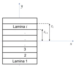
Figure 1.2 Multiple laminae stacked onto each other to from a laminate, which
in turn is part of composite structure . . . 13
Figure 1.3 Ply number system . . . 16
Figure 1.4 Straight-crested waves in a plate: (a) the different type of
straight-crested waves [21]; and (b) the different Lamb waves in
a plate . . . 18
Figure 1.5 Schematic representation of the particle motion for the
shear-horizontal wave mode . . . 20
Figure 1.6 Schematic representation of the particle motion for the: (a,b)
symmetric Lamb wave mode; and (c,d) anti-symmetric Lamb wave mode 22
Figure 4.1 Schematic representation of the axes x1 and x3 used in the UAM
formulation . . . 38
Figure 4.2 Schematic representation of an N-layered medium and the
corresponding variables . . . 43
Figure 4.3 Schematic representation of a three-layered medium and the
corresponding variables used to elaborate the TMM . . . 45
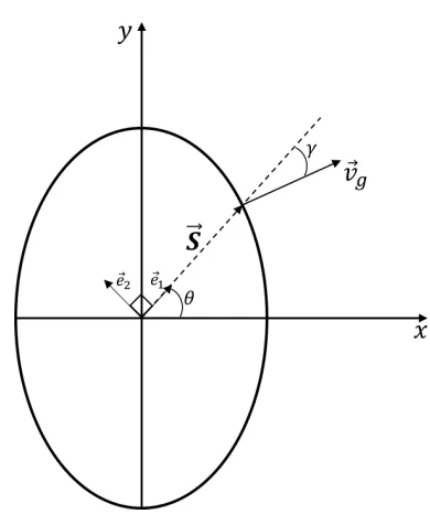
Figure 4.4 Schematic of the geometric relation between slowness vector and
group velocity vector . . . 53
Figure 4.5 Schematic of the geometric relation between slowness vector, group
velocity vector and steering angle . . . 56
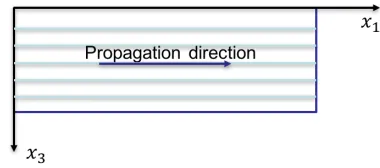
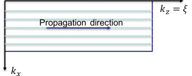
Figure 5.1 Schematic representation of the axes kx and kx used in the
Figure 5.2 Schematic representation of the axesx, y andz used in the SAFE
formulation [26] . . . 63
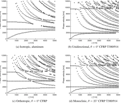
Figure 6.1 α2 behavior for different types of material, one layer 1 mm in
thickness: (a) isotropic, aluminum; (b) unidirectional, θ = 0° CFRP T300/914; (c) orthotropic,θ = 0° CFRP; and (d) monoclinic,
θ= 25° CFRP T300/914 . . . 69
Figure 6.2 Illustration of the phase change approach, (a) initial complex
number represented by its phaseθi, and (b) consecutive phaseθi+1
when sign change was recorded. . . 76
Figure 6.3 Dispersion curves obtained using the phase approach in a 1 mm
thick plate: (a) isotropic, aluminum; (b) orthotropic transversely isotropic, θ = 0° CFRP T300/914; (c) fully orthotropic, θ = 0°
CFRP; and (d) monoclinic,θ = 25° CFRP T300/914 . . . 77
Figure 6.4 Modeshape for the fundamental waves for an orthotropic material at
aξof 810/m: (a)A0; (b)S0; (c)SHA0; and (d)SHS0 . . . 79
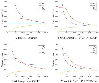
Figure 6.5 Dispersion curves after modeshape analysis and spline algorithm
in a 1 mm thick plate: (a) isotropic, aluminum; (b) orthotropic transversely isotropic,θ = 0° CFRP T300/914; (c) fully orthotropic,
θ= 0° CFRP; and (d) monoclinic,θ = 25° CFRP T300/914 . . . 80
Figure 6.6 Dispersion curves for 50-layer 1 mm thick laminate using GMM
and TMM respectively: (a,b) isotropic; (c,d) fully orthotropic . . . 82
Figure 6.7 Dispersion curves for 1 mm thick laminate using GMM and TMM
respectively: (a,b) quasi-isotropic[45/−45/0/90]s; and (c,d) fiber
metal laminate, orthotropic/isotropic[0/0]s . . . 83
Figure 6.8 The effect of the number of element through the thickness on
the accuracy of the SAFE solution compared to the UAM for an
aluminum 1 mm thick plate . . . 84
Figure 6.9 Dispersion curves obtained the UAM, SAFE method and
DISPERSE for a single 1 mm thick layer (a) isotropic, aluminum; (b) unidirectional CFRP; (c) orthotropic CFRP; and (d) monoclinic,
Figure 6.10 Dispersion curves obtained the UAM, SAFE method and DISPERSE for a multi 10 layered (a) isotropic, aluminum; (b) unidirectional CFRP; (c) orthotropic CFRP; and (d) monoclinic,
θ= 45° CFRP . . . 86
Figure 6.11 Dispersion curves obtained the UAM, SAFE method and
DISPERSE for a laminate: (a) [0/90]; (b) [0/45/90]s; (c)
[±45/0/90]s; and[±45/Al/90]s . . . 88
Figure 6.12 Dispersion curves obtained the UAM, SAFE method and
DISPERSE for a sandwich laminate . . . 89
Figure 6.13 Group velocity dispersion curves obtained using the energy velocity approach in a 1 mm thick plate: (a) isotropic, aluminum; (b) orthotropic transversely isotropic,θ= 0° CFRP T300/914; (c) fully
orthotropic,θ = 0° CFRP; and (d) monoclinic,θ= 45° CFRP T300/914 91
Figure 6.14 Dispersion curves obtained the UAM, SAFE method and
DISPERSE for a laminate: (a) [0/90]; (b) [0/45/90]s; (c)
[±45/0/90]s; and (d)[±45/Al/90]s . . . 92
Figure 7.1 The effect of discretization step size in the phase velocity domain for a 1mm thick aluminum plate. A step size of: (a) 100 m/s; (b) 10
m/s; (c) 1 m/s; and (d) 0.1 m/s . . . 94
Figure 7.2 Conversion from wavenumber to frequency domain: (a)
fundamental wavenumber-phase velocity domain; and (b)
frequency-phase velocity domain corresponding to the conversion
of (a) . . . 95
Figure 7.3 Conversion from wavenumber to frequency domain for a 1mm
thick aluminum plate with a step size of 0.1 m/s in the phase velocity domain: (a,b) wavenumber domain set to 5010/m; and (c,d)
wavenumber domain set to 6810/m . . . 96
Figure 7.4 Comparison between dispersion curves obtained form frequency as
fundamental variable: (a) isotropic, aluminum 1 mm thick plate;
and (b) unidirectional CFRP 1 mm thick plate . . . 98
Figure 7.5 Unidirectional CFRP 1 mm thick plate dispersion curves obtained
with wavenumber as fundamental variable: (a) wavenumber domain range of 8010/m; and (b) frequency domain after conversion from
Figure 7.6 Conversion from frequency to wavenumber domain:
(a) fundamental frequency-phase velocity domain; (b)
wavenumber-phase velocity domain corresponding to the
conversion of (a); and (c) wavenumber-phase velocity domain (b) restricted to a maximum 5010/m. Note the difference in x-axis
scale: [1/mm] in (b); and [1/m] in (c) . . . 99
Figure 7.7 Evaluation of the TMM for high wavenumbers: (a) isotropic
aluminum, no numerical instability observed; and (b) unidirectional
CFRP ,numerical instability observed around 7000/m . . . 100
Figure 7.8 Evaluation of the TMM for high wavenumbers: (a) unidirectional
CFRP at an orientation angle of 0°; (a) unidirectional CFRP at an orientation angle of 75°; and (c) orthotropic CFRP at an orientation
angle of 0° . . . 101
Figure 7.9 The fundamental waves: (a) before separation and grouping; and (b)
after separation and grouping . . . 102
Figure 7.10 Modeshape for the fundamental waves for an isotropic material at a
wavenumber of: (a,b,c,d) 1510/m; (e,f,g,h) 1610/m; and (i,j,k,l) 1710/m 103
Figure 7.11 The effect of the number of points through the thickness on the group velocity calculations: (a) 21 points; (b) 51 points; (c) 101
points; (d) 251 points; (e) 501 points; and (f) 1001 points . . . 105
Figure 7.12 Group velocity calculated: (a) using a phase velocity accuracy of 1 m/s and 1001 points through the thickness; (b) using a phase velocity accuracy of 0.1 m/s and 1001 points through the thickness;
(c) zoom in of (a); and (d) zoom in of (b) . . . 106
Figure 7.13 Group velocity for the frequency domain using 101 points through
the thickness . . . 107
Figure 7.14 The phase velocity for a CFRP unidirectional at various orientation
angleθand corresponding steering angle: (a,b)θ=0°; and (c,d)θ=10° . 108
Figure 7.15 The phase velocity for a CFRP unidirectional at various orientation
angleθand corresponding steering angle: (a,b)θ=40°; and (c,d)θ=73° 109
Figure 10.1 Different ultrasonic immersion technique method: (a)
through-transmission method and (b) double through-transmission . . . 127
Figure 10.3 Ultrasonic immersion technique rotation angles: (a) in-plane
rotationφ; and (b) out-of-plane rotationθi . . . 128
Figure 10.4 Elastic constants, reference axes and planes of propagation of ultrasonic waves for orthotropic material elaborated in the form of
thin plate [19] . . . 129
Figure 10.5 Kriz and Stinchcomb’s approach: (a) experimental setup; and
(b)specimen dimensions [14] . . . 131
Figure 10.6 Wave propagates on the surface at the critical angleθcr . . . 134
Figure 10.7 Experimental setup for the ultrasonic immersion technique: (a)
isometric view (b) front view . . . 135
Figure 10.8 C-scan measurement used to determine the center of theyandzlocations136
Figure 10.9 The maximum absolute peak amplitude for each incident angle and
y-location prior to correcting the offsets . . . 138
Figure 10.10The maximum absolute peak amplitude in the: (a)y-direction; and
(b) the range of incident angles . . . 138
Figure 10.11The maximum absolute peak amplitude for each incident angle and
y-location after correcting the offsets . . . 139
Figure 10.12Extraction of ToF from data illustrated: (a) normalized signal; (b)
envelope of signal; and (c) threshold used to determine ToF . . . 140
Figure 10.13Determining the difference in ToF: (a) normalized pulse-echo
signal; and (b) illustration to derive∆t . . . 141
Figure 10.14Data extraction results: (a) ToF; (b) change in ToF,∆t; and (c) phase
velocity . . . 142
Figure 10.15Flowchart inverse problem routine . . . 143
Figure 10.16Two basins of attraction with two different final points [21] . . . 143
Figure 10.17Data from the (x1,x3)-plane of symmetry for each incident angleθi: (a) maximum absolute peak amplitude in eachy-location; (b) phase velocity for full incident angle range; (c) phase velocity for reduced
Figure 11.1 MTS machine used for experiments . . . 153
Figure 14.1 The composite cutout placed in the ultrasonic immersion water tank . . 170
Figure 14.2 Time-of-flight data from the composite cutout: (a) pristine cutout
prior to impact; and (b) damaged cutout after cutout . . . 172
Figure 14.3 Amplitude data from back surface gate of the composite cutout: (a)
pristine cutout prior to impact; and (b) damaged cutout after impact . . . 173
Figure 14.4 Amplitude data from back surface gate of the composite cutout: (a)
pristine cutout prior to impact; and (b) damaged cutout after cutout . . . 174
Figure 14.5 Olympus introduces the RollerFORM setup . . . 175
Figure 14.6 C-scan of impact location: (a) prior to impact; (b) after an impact of 5 Joules; and (c) after an impact of 9 Joules. Note, the cross
indicates the impact location . . . 177
Figure 14.7 Through the thickness measurement corresponding to an impact of
5 Joules using the Olympus hand-held phased array scanner . . . 177
Figure 15.1 NASA unidirectional CFRP M7G-8552 plate with PWAS bonded
onto it . . . 179
Figure 15.2 Data from the (x1,x3)-plane of symmetry for each incident angle
θi: (a) maximum absolute peak amplitude in each y-location; (b) difference in ToF for the incident angle range; (c) phase velocity for
the incident angle range . . . 180
Figure 15.3 Data from the (x2,x3)-plane of symmetry for each incident angle
θi: (a) maximum absolute peak amplitude in each y-location; (b) difference in ToF for the incident angle range; (c) phase velocity for
the incident angle range . . . 181
Figure 15.4 Comparison the maximum absolute peak amplitude of the data in the (x1,x3)-plane of symmetry for each incident angleθi: (a) for a
3.30 mm thick specimen; and (b) for a 16.43 mm thick specimen . . . . 182
Figure 15.5 Experimental result from the destructive mechanical testing procedures: (a) stress versus strain curve to determineE11; and (b)
Figure 15.6 Thermoplastic 5-Harness carbon/PPS fabric plate with PWAS
bonded onto it . . . 187
Figure 15.7 Pulse-echo measurement to determine C33 for the thermoplastic
5-Harness carbon/PPS fabric composite . . . 187
Figure 15.8 Data from the (x1,x3)-plane of symmetry for each incident angle
θi: (a) maximum absolute peak amplitude in each y-location; (b) difference in ToF for the incident angle range; (c) phase velocity for
the incident angle range . . . 189
Figure 15.9 Data from the (x2,x3)-plane of symmetry for each incident angle
θi: (a) maximum absolute peak amplitude in each y-location; (b) difference in ToF for the incident angle range; (c) phase velocity for
the incident angle range . . . 190
Figure 15.10Data from the non-symmetric plane (45°) for each incident angle
θi: (a) maximum absolute peak amplitude in each y-location; (b) difference in ToF for the incident angle range; (c) phase velocity for
the incident angle range . . . 191
Figure 16.1 Schematic illustration of the hybrid PWAS-SLDV system
experimental setup . . . 194
Figure 16.2 The SLDV response for 1 mm aluminum plate example; time, distance and particle velocity amplitude in: (a) isometric view and
(b) 2D time-distance view . . . 195
Figure 16.3 Comparison between experimental and predicted
wavenumber-frequency dispersion curves for 1 mm aluminum plate example; experimentally SLDV response after post-processing
versus UAM prediction . . . 196
Figure 16.4 Unidirectional plate used for the validation process (15.25-mm
IM7G-8552 unidirectional 96-ply composite) . . . 197
Figure 16.5 The SLDV response for IM7G-8552 unidirectional 96-ply composite plate; time, distance and particle velocity amplitude in:
(a) isometric view and (b) 2D time-distance view . . . 197
Figure 16.6 Comparison between experimental and predicted
wavenumber-frequency dispersion curves for IM7G-8552
unidirectional 96-ply composite plate; experimentally SLDV
Figure 16.7 Comparison between experimental and predicted
wavenumber-frequency dispersion curves for IM7G-8552
unidirectional 96-ply composite plate; experimentally SLDV
response after post-processing versus UAM prediction using material properties obtained using mechanical testing and LAMSS
ultrasonic method . . . 199
Figure 16.8 Comparison between experimental and predicted
wavenumber-frequency dispersion curves for IM7G-8552
unidirectional 96-ply composite plate; experimentally SLDV
response after post-processing versus UAM prediction using material properties through the LAMSS ultrasonic method for a
thick (16.43 mm) and thin (3.30 mm) specimen . . . 200
Figure 16.9 The SLDV response for the thermoplastic 5-Harness carbon/PPS fabric 24-ply composite plate; time, distance and particle velocity
amplitude in: (a) isometric view and (b) 2D time-distance view . . . 201
Figure 16.10Comparison between experimental and predicted
wavenumber-frequency dispersion curves for thermoplastic
5-Harness carbon/PPS fabric 24-ply composite plate;
experimentally SLDV response after post-processing versus
UAM prediction . . . 202
Figure 16.11Comparison between experimental and predicted
wavenumber-frequency dispersion curves for thermoplastic
5-Harness carbon/PPS fabric 24-ply composite plate;
experimentally SLDV response after post-processing versus UAM prediction using material properties obtained using mechanical
testing and LAMSS ultrasonic method . . . 204
Figure A.1 Schematic representation of a unidirectional material . . . 217
Figure A.2 Stress transformations on the plane of isotropy . . . 219
Figure A.3 Axis rotations in the plane of isotropy . . . 219
Figure B.1 Unified analytic method flowchart . . . 224
Figure D.1 Illustration of difference in acoustic paths for propagation with
Figure D.2 Illustration of difference in acoustic paths for propagation with
phase velocity vp and group velocity vg when using the
S
UMMARY
In the aerospace industry, non-destructive evaluation (NDE) techniques are used to
maintain safety and integrity of components, parts, and structures. Various methods (e.g.
visual inspection, liquid penetrant testing, magnetic particle testing, ultrasonic testing,
thermal infrared, etc.) exist within the field of NDE. Methods based on ultrasonics however
are often preferred due to their merits (e.g. high sensitivity, thickness information as output,
etc.); ultrasonic guided-waves (GW) are commonly used (in laboratory enviroment) due
to their ability to travel over long distances. Therefore, it is of great value to know the
characteristics of these ultrasonic GW, e.g. the wave and group velocity in the propagating
medium. For ultrasonic GW which are dispersive (the propagation velocity is dependent
on the excitation frequency) it is of importance to model and measure the dispersion curves
accurately. In addition, it is important to state that, current NDE methods were developed
with metals in mind, prior to applying these methods to composite materials more research
is required.
Current practice is to use different solution approaches to predict the dispersion curves
based on the material of the medium in which the ultrasonic GW propagate. In addition, the
different solution approaches are defined in different domains, frequency-phase velocity
domain for isotropic materials and wavenumber-phase velocity domain for anisotropic
materials, this may can lead to difficulties and unsatisfying results when predicting
the dispersion curves for hybrid laminates which contain both isotropic and anisotropic
materials. A unified formulation defined in the wavenumber-phase velocity domain for
both isotropic and anisotropic materials was therefore developed. The unified analytic
method (UAM) is a simple and mathematically straightforward formulation, that utilized
eigenvalues and eigenvectors are used to set up the field matrix from which the dispersion
curves can be retrieved using the phase approach. Once the dispersion curves are obtained
the waves are grouped based on their modeshape using a modeshape analysis technique.
The modeshape analysis was successfully applied to the fundamental wave modes (S0,A0,
SHS0andSHA0). Once the waves were grouped, a spline algorithm was applied to obtain
a continuous solution for the dispersion curves in the desired domain.
A comparative study between a commercially available dispersion curve package
called DISPERSE, the semi-analytic finite element (SAFE) approach, and the UAM was
performed to verify the accuracy of the obtained solution. The dispersion curves were
compared for four different cases: (i) single layer; (ii) multi-layer (all the layers are
orientated in the same direction); (iii) laminates (layers can have different orientations);
and (iv) sandwich laminate (a laminate that has a core made out of foam or honeycomb
material; sandwich laminate are significantly thicker on average). For the first two cases,
the investigated materials were: (i) isotropic; (ii) unidirectional; (iii) orthotropic; and (iv)
monoclinic material. The laminate cases had the following stacking sequences: (i)[0/90]; (ii)[0/45/90]s; (iii) [±45/0/90]s; and (iv) [±45/Al/90]s. It is important to note that the fourth case is a combination of isotropic and anisotropic material, i.e. a fiber metal laminate
(FML). This case was selected to highlight that UAM is capable to retrieve the dispersion
curves in a medium that consist of multiple materials. In addition, the sandwich case was
used to investigate the performance of UAM in large thickness media. In all cases, the
UAM provided as accurate or better set of dispersion curves when compared to the results
obtained by DISPERSE and SAFE. It is important to state that, the comparison between
UAM, DISPERSE, and SAFE was made for materials with a known the stiffness matrix.
To validate the UAM, an accurate stiffness matrix of the propagating medium is
required. To determine the stiffness matrix, it is common practice to use the standard
mechanical testing procedures set by ASTM International (to determine the Young’s
ratio in 12-direction) in combination with assumptions based on the material type, e.g.,
for unidirectional materials, the Young’s modulus in the 3-direction equals that in the
2-direction. When using this approach, the predicted dispersion curves vary significantly
from those obtained experimentally using a piezoelectric wafer active sensor (PWAS)
excitation and scanning laser Doppler vibrometer (SLDV) measurements. The source of
error was identified to be the accuracy of the stiffness matrix, therefore a different and more
accurate method to determine the stiffness matrix was desired. In this research, the stiffness
matrix components were determined non-destructively using a novel ultrasonic immersion
technique, the LAMSS ultrasonic immersion technique. Results showed that the two
methods (destructive mechanical testing versus LAMSS ultrasonic immersion technique)
differed when comparing the stiffness matrices directly. To determine which method
yielded the more accurate results, the dispersion curves were compared to experimentally
obtained dispersion curves using the hybrid PWAS-SLDV setup. For both a unidirectional
plate and a woven fabric composite plate, the stiffness matrix retrieved using the LAMSS
ultrasonic immersion technique yielded more accurate GW results than those obtained with
Part I
NOMENCLATURE
Abbreviation Description
2D 2-dimensional
3D 3-dimensional
AE Acoustic emission
BMI Bismaleimidi
CLT Classical laminate theory
ET Eddy current testing
FFT Fast Fourier transform
FML Fiber metal laminate
GMM Global matrix method
GW Guided-waves
MPT Magnetic particle testing
NDE Non-destructive evaluation
PT Penetrant testing
PWAS Piezoelectric wafer active sensor
RT Radiographic testing
SAFE Semi-analytic finite element
SH Shear-horizontal
SHM Structural health monitoring
SLDV Scanning laser Doppler vibrometer
SMM Stiffness matrix method
STMM Stiffness transfer matrix method
TiR Thermal infrared testing
TMM Transfer matrix method
UT Ultrasonic testing
VT Visual testing
Arabic letter Description Unit
A Membrane stiffness matrix Pa
B Out-of-plane in-plane coupling matrix Pa
C Stiffness matrix Pa
D Bending stiffness matrix Pa
E Young’s modulus Pa
G Shear modulus Pa
h Plate thickness m
k Wavenumber m−1
M Moment resultants Nm
N In-plane stress resultants Pa
Q Reduced stiffness matrix Pa
Q Transformed stiffness matrix Pa
T Transformation matrix
vL Longitudinal velocity ms−1
vS Shear velocity ms−1
vT Transverse velocity ms−1
Greek letter Description Unit
Strain
λ Lamé constant
λwave Wavelength m
µ Shear modulus Pa
σ Normal stress Pa
τ Shear stress Pa
C
HAPTER
1
P
REAMBLE
Modern aircraft have dramatically evolved from their ancestor the wood and linen Wright
Flyer to modern day composite aircraft the Airbus A350XWB. A picture of the maiden
flight to the Wright Flyer1 and that of the Airbus A350XWB2 is given in Fig. 1.1 to
highlight the chances. While the Wright Flyer was made mostly out of wood and linen,
nowadays metal alloys and composites are the most used materials in an aircraft. Besides
the change in materials used, the design methodologies, testing procedures, and safety
regulation have evolved drastically as well.
(a) (b)
Figure 1.1: The maiden flight of the: (a) Wright Flyer courtesy of the United States Library of Congress; and (b) Airbus A350XWB courtesy of Airbus
This chapter starts with a concise overview of the history of aviation and non-destructive
evaluation (NDE) techniques. Second, the motivation for this research is elaborated upon.
Finally, the dissertation hypothesis are presented and elaborated.
1.1 HISTORY OF AVIATION AND NON-DESTRUCTIVE EVALUATION(NDE)
The current state of the aerospace industry is achieved by accumulated progress that
started before3 the Wright brothers and their Wright Flyer and still is continuing today.
A brief overview of major milestones [1] in the history of aviation is listed below in a
chronological order for the reader’s convenience.
1905 1910 1915 1920 1925 1930 1935 1940 1945
1799, Sir
Geor geCayle
y
Wright brothers
DeperdussinFokk er
Hugo Junck
ers
Lockheed Vega
Boeing 247
Douglas DC-2
and DC-3
1950 1955 1960 1965 1970 1975 1980 1985 1990 1995 2000 2005 2010
deHa villand
DH 106
Comet
Aérospatiale/B AC
Concorde
Introduction
ofcomposites
Learf an
Beechcraft Starship
Boeing B787
On December 17, 1903, when the Wright brothers took to the skies in their Wright
Flyer, the materials used where wood, steel wire, and linen.
In 1912, Deperdussin replaced the load carrying struts and bars with a load carrying
fusalage, the monocoque fuselage; however, wood remained the primary material of the
aircraft. One year later, in 1913, Fokker introduced an aircraft for which the load carrying
fuselage was made out of steel tubes instead of wood; this was succeeded in 1916 by the
first all metal aircraft, the Junckers J1. The J1 model was made out of steel which made
it heaver than its wooden counterpart, however this disadvantage was later overcome by
changing the choice of material to an aluminum-copper alloy known as duralumin which
was used in the J4 model.
The development of all metal aircraft accelerated in the 1930’s after the crash of the
31799, Sir George Caylay; separation of lift generation and powerplant is one of the most important
Fokker F10 Trimotor, a crash that discredited the adhesively bonded wooden wings aircraft.
In 1931, Boeing introduced the first metal passenger aircraft, the Boeing 247, a twin-engine
monoplane aircraft. Douglas Aircraft Corporation responded with the Douglas DC-2 in
1934 and its larger version the DC-3 in 1935 which became one of the most successful
aircraft and set the standard for metal aircraft structure.
During the second world war, wooden aircraft got a revival due to the shortage of
aluminum; the Mosquito bomber and Beriev Be-2 reconnaissance flying boat are examples
of wooden aircraft developed and manufactured during the second world war. After
the second world war, the focus shifted towards improving the aircraft performance
and passenger comfort since civil transportation became more important for aircraft
manufacturers. More powerful engines and the introduction of the pressurized fuselage
made it possible for aircraft to fly into the top of the troposphere/low stratosphere (e.g.,
Boeing 377 Stratocruiser); possible for aircraft to fly above the clouds and weather
conditions while keeping the cabin pressure at a reasonable level. The first jet engines
allowed for even faster travel and at higher altitudes.
To fly above the weather while maintaining a reasonable cabin pressure required
pressurizing and depressurizing of the cabin. This pressurizing and depressurizing cycle
on the fuselage for each flight caused fatigue related problems. Accidents with the de
Havilland Comet which where attributed to fatigue in combination with bad design features
and incorrect testing of the aircraft4 lead to strict design and test regulations to prevent
future accidents.
The next major leap forward (ignoring the Concorde, the first supersonic passenger
aircraft) was the introduction of composite components into the aircraft. Initially,
composites were used only in secondary and non-load carrying components such as fairings
and the radome. Over the last decades, however, composite components have gradually
4The ultimate load was applied before the fatigue testing, this lead to fatigue initiation to occur later than
replaced their metal counterparts even in primary structural components. The Boeing
B787 and Airbus A350XWB are examples of modern passenger aircraft that by percentage
weight more than 50% is composite material.
Alongside the aforementioned milestones, progress was made in the techniques for
testing and quantifying the strength of aircraft. Mechanical testing (to measure ultimate
tensile strength, yield point of the material, fatigue life, toughness etc.) were conducted
to quantify the materials used in the design phase and eventually for manufacturing.
To maintain the in-service aircraft integrity, mechanical testing (due to their destructive
nature) is no longer an option; therefore, NDE techniques were required. A comprehensive
overview of the major NDE techniques as given by Hellier [2] are presented in Tab. 1.1.
The NDE techniques listed in Tab. 1.1 were developed with isotropic and homogeneous
materials in mind, however, composite materials (anisotropic non-homogeneous) started
gradually replacing metallic materials in critical components of civil transport aircraft
structures since the 1980s; and more recently, both Boeing (B787) Airbus (A350XWB)
have manufactured aircraft which mostly is made of composites. In contrast to metallic
structures, low energy impact damage in composite structures can create damage beneath
the surface not visible externally to the naked eye. The low energy impacts can result
in delaminations, fiber breakage, and/or matrix cracking which may lead to a significant
decrease of the material strength and reduce the structure’s fatigue life [3, 4]. Even though
some current NDE techniques (i.e., using an ultrasonic water tank to perform a C-scan) are
capable to capture the effect of low energy impact, they remain expensive for the aircraft
operator both in time and costs. To reduce downtime of an aircraft, and to lower the cost
of maintenance, while at the same time increasing our knowledge on the structural health,
a different method of damage detection is needed; an integrated NDE system that can
evaluate the state of a component in-service without the need to ground the aircraft for
a scheduled maintenance. The field of research aim to accomplish the aforementioned is
Table 1.1: Major NDE techniques; a comprehensive overview [2]
Technique Principle Application Advantages Limitations
Visual testing (VT)
Uses reflected or transmitted light from test object that is imaged with the human eye or other light-sensing device
Many applications in many industries ranging from raw material to finished products and in-service inspection
Can be inexpensive and simple with minimal training required. Broad scope of uses and benefits
Only surface conditions can be evaluated. Effective source of illumination required. Access necessary
Penetrant testing (PT)
A liquid containing visible or fluorescent dye is applied to surface an enter discontinuities by capillary action
Virtually any solid nonabsorbent material having uncoated surface that are not contaminated
Relatively easy and material are inexpensive. Extremely sensitive, very versatile. Minimal training
Discontinuities open to the surface only. Surface conditions must be relatively smooth and free of contaminant Magnetic
particle testing (MPT)
Test part is magnetized and fine ferromagnetic particles applied to surface, aligning at discontinuity
All ferromagnetic materials, for surface, and slightly subsurface discontinuities; large and small parts
Relatively easy to use. Equipment/material usually inexpensive. Highly sensitive and fast compared to PT.
Only surface and a few subsurface discontinuities can be detected. Ferromagnetic materials only Radiographic
testing (RT)
Radiographic film is exposed when radiation passes through the test object. Discontinuities affect exposure
Most materials, shapes and structures. Examples include welds, castings, composites, etc. as manufactured or in-service
Provides a permanent record and high sensitivity. Most widely used and accepted volumetric examination
Limited thickness based on material density. Orientation of planar discontinuities is critical. Radiation hazard
Ultrasonic testing (UT)
High frequency sound pulses from a transducer propagate through the test material, reflecting at interfaces
Most materials can be examined if sound transmission and surface finish are good and shape is not complex
Provides precise, high sensitivity results quickly. Thickness information, depth and type of flaw can be obtained from one side of the component
No permanent record (usually). Material attenuation, surface finish and contour. Requires couplant
Eddy current testing (ET)
Localized electrical fields are induced into a conductive test specimen by electromagnetic induction
Virtually all conductive material can be
examined for
flaws, metallurgical conditions, thinning and conductivity
Quick, versatile, sensitive; can be non-contacting; easily adaptable to automation and in-situ examination
Variables must
be understood
and controlled. Shallow-depth of penetration, lift-off effects and surface condition
Thermal infrared testing (TIR)
Temperature variations at the test surface are measured/detected
using thermal
sensors/detectors instruments/cameras
Most materials and components where temperature changes are related to part conditions/thermal conductivity
Extremely sensitive to slight temperature changes in small parts or large areas. Provides permanent record
Not effective for detection of flaws in thick parts. Surface only is evaluated. Evaluation requires high skill level
Acoustic emission testing (AE)
As discontinuities propagate, energy is released and travels as stress wave through the material. These are detected by means of sensors
Welds, pressure vessels, rotating equipment, some composites and other structures subject to stress or loading
Large areas can be monitored to detect deteriorating conditions. Can possibly predict failure
be distinguished: (i) load monitoring, in which the load cycles of a component is recorded
and based on the load history and a fatigue based model the remainder of life is estimated;
and (ii) damage assessment, aimed at the development of integrated systems which are
capable to detect and monitor damage in aircraft structures in-situ [5] In combination with
the increase in understanding of smart materials, and the decrease in size of sensors, SHM
systems are becoming more feasible. Furthermore, integrating SHM sensors onto (bonded),
or into (in / embedded) the structure makes NDE techniques a part of the whole structure.
This gives the operators the opportunity to inspect the aircraft before each flight, or during
a flight. The aircraft would only need to be put out of service when damage is detected, no
longer after a certain, defined period or number of flights [6].
For SHM purpose, ultrasonic guided-waves (GW), more specific Lamb waves [7], are
preferred due to their capability to travel long distances [8]. To obtain/develop accurate
SHM system, however, an increase of knowledge and more accurate predictive models
of ultrasonic GW propagation (dispersion curves) in an arbitrary material and realistic
structure is necessary. Current GW based techniques are limited to simple geometries
(such as flat or curved plates), prior to the implementation of a GW based system in an
aircraft, complex geometries (changes in thickness, stiffeners, ribs, fasteners, etc.) have
to be investigated. However, this work aims on the fundamental principles of GW and is
limited to simple geometries.
The aim of this dissertation is to contribute to existing literature through: Part II:
propose a unified formulation (unified analytic method, UAM) that predicts ultrasonic GW
propagation in any material type or combination of materials and verify this method by
comparison with existing dispersion curves algorithms; Part III: retrieve the stiffness matrix
(which acts as input for the UAM) non-destructively using the newly formulated LAMSS
ultrasonic immersion technique with increased accuracy. A stiffness matrix determined
through destructive mechanical testing and based on material assumptions will not yield
matrix and predicted dispersion curves experimentally using a piezoelectric wafer active
sensor (PWAS) exciter and ascanning laser Doppler vibrometer (SLDV) to measure GW
propagation in unidirectional and fabric composites.
1.2 HISTORY OF ULTRASONIC GUIDED-WAVES (GW)
Propagation of elastic waves was first investigate by Rayleigh [9] in 1885, who was
interested in modeling the motion of the ground due to earth tremors. Rayleigh’s work
(solving the wave equation using one traction-free boundary) on elastic waves traveling on
the free surface of a semi-infinite solid formed the foundation of all future work in this area.
In 1911, Love [10] continued Rayleigh’s work by investigating wave propagation in a finite
thickness layer and solved it for the shear-horizontal (SH) wave case. In 1917, Lamb [7]
investigated the wave propagation in a layer with two traction-free boundaries. Lamb
concluded that two types of wave modes exist simultaneously, one symmetric- and one
antisymmetric. Stoneley [11] continued Rayleigh’s work and generalized the formulation
for the interface of two semi-infinite solids. Stoneley’s generalized formulation was used
by Scholte [12] to investigate wave propagation at the interface of two semi-infinite media
when one of them was water.
1885 1890 1895 1900 1905 1910 1915 1920 1925 1930 1935 1940 1945 1950
Rayleigh Love Lamb Stonely Scholte
The pioneering and fundamental work described above mostly focused on geophysical
systems; the first significant study on elastic wave propagation in multi layered media
was performed by Thomson [13]. Three year later, Haskell [14] corrected a minor error
in Thomson’s work. The method described by Thomson and Haskell used a recursive
algorithm to obtain a compact matrix (transfer matrix method, TMM) in which the
boundary conditions of all the layers were eventually related to the boundary conditions
to determine the dispersion curves.
Knopoff [15] formulated a direct approach in which the boundary conditions of all
layers are assembled into one matrix. Knopoff’s global matrix method (GMM) is more
stable than the TMM used by Thomson and Haskell, however the global matrix increases
in size with an increasing number of layers.
An alternative to the GMM and TMM was presented by Rokhlin and Wang [16, 17] in
which the stresses are related to the displacements at the surfaces of the media. Rokhlin
and Wang’s stiffness matrix method (SMM) is considered to be unconditionally stable.
In addition to aforementioned methods, Kamal [18] introduced the stiffness transfer
matrix method (STMM) that combines the merits of both the TMM and SMM into one
method.
1955 1960 1965 1970 1975 1980 1985 1990 1995 2000 2005 2010 2015
ThomsonHask ell
Knopof f
Viktoro v
Lowe; Nayfeh
etal.
Pavlak ovic
Rokhlin, Wang
and Yuan
Bartoli etal.
Wang and
Yuan
GopalakrishnanKamal
1.3 COMPOSITES
A composite material consists out of two or more constituent materials which combine
produce a material with properties different from the individual components. Often
mistaken to be a new material, the opposite is more true since composite materials can
be traced back to Ancient Egypt when mud and straw were combined to produce bricks;
another commonly used composite material is concrete.
However, the aforementioned will not do for aerospace structures; the composite
materials used in the aerospace industry can be a combination of carbon or glass fiber
and a matrix of epoxy-, Bismaleimidi- (BMI) or thermoplastic- resin, etc.5. The fibers are
the major load carrying members, while the matrix is used to protect the fiber from the
environment and the transfer loads to and between the fibers.
A ply or lamina refers to a sheet of fibers and matrix; stacking multiple plies or laminae
on each other one creates a laminate. Laminates can consists out multiple layers each in a
desired orientation to produce a composite with desired properties. E.g. a laminate with an
equal distribution of plies in the 0°, 90° and±45° will result in a quasi-isotropic laminate, a
laminate with stiffness properties similar to isotropic (metallic) materials; the properties are
independent of rotation of the axis system. The composite laminates in turn can be used
to produce composites structures such a fuselage section, wingbox, etc.; a process from
lamina to laminate to structures is schematically represented in Fig. 1.2. In other methods,
such as automated fiber placement, the uncured composite material is placed directly into
the final structural shape by using a mold.
(a) Lamina (b) Laminate (c) Composite structure
Figure 1.2: Multiple laminae stacked onto each other to from a laminate, which in turn is part of composite structure
CLASSICAL LAMINATE THEORY
Classical laminate theory (CLT) forms the foundation for mechanical analysis of
composites; in this section, a brief introduction is provided for the reader’s convenience;
however, it is recommended the books by Daniels [19] and Kassapoglou [4] (just to name
a few) for more detailed information.
principal axes can be related to the strains using the following constitutive equations σ1 σ2 τ12 =
Q11 Q12 0
Q22 0
sym Q66
1 2 γ12 (1.1)
whereQij is defined by
Q11=
E1
1−ν12ν21
,Q12=
ν21E1
1−ν12ν21
,Q22=
E2
1−ν12ν21
,Q66=G12 (1.2)
The aforementioned relations describe the stiffness properties of a lamina in the principal
directions and the material propertiesE1,E2,G12andν12. It is common for the principal
axis not to coincide with the loading directions, or reference axis. To express the stiffness
properties in the principal directions in terms of the loading axis, the x-, y-coordinate
system, the following transformation has to be applied to the stresses and strains
σx σy τxy
= [T2D]
σ1 σ2 τ12 (1.3) x y 1 2γxy
i
= [T2D]
1 2 1 2γ12
i (1.4)
whereT2D is given by
[T2D] =
m2 n2 2mn n2 m2 −2mn
−mn mn (m2−n2)
(1.5)
where m = cos(θ), n = sin(θ), and θ is the orientation angle of the lamina. Using
obtains σx σy τxy
= [T2−D1]
Q11 Q12 Q16
Q22 Q26
sym Q66
[T2D]
x y 1 2γxy
(1.6)
One can now define
Q11 Q12 Q16
Q22 Q26
sym Q66
= [T2−D1]
Q11 Q12 Q16
Q22 Q26
sym Q66
[T2D] (1.7)
whereQij is given as
Q(11θ) =m4Q11+n4Q22+ 2m2n2Q12+ 4m2n2Q66
Q(22θ) =n4Q11+m4Q22+ 2m2n2Q12+ 4m2n2Q66
Q(12θ) =m2n2Q11+m2n2Q22+ (m4+n4)Q12−4m2n2Q66 (1.8)
Q(66θ) =m2n2Q11+m2n2Q22−2m2n2Q12+ (m2−n2)2Q66
Q(16θ) =m3nQ11−mn3Q22+ (mn3−m3n)Q12+ 2(mn3−m3n)Q66
Q(26θ) =mn3Q11−m3nQ22+ (m3n−mn3)Q12+ 2(m3n−mn3)Q66
The in-plane stress resultants, and moments resultants are defined as
Ni =
Z h
2
−h
2
σidz Mi =
Z h
2
−h
2
σizdz (1.9)
whereNiare the in-plane stress resultants andMiare the moment resultants in theith-layer
of the laminate. Utilizing Eq. (1.6) to Eq. (1.9) one obtains
N =A·+B ·κ
whereA,B, andDare given by
Aij = n
X
i=1
(Qij)i(zk−zk−1)
Bij =
1 2
n
X
i=1
(Qij)i(zk2−z 2
k−1) (1.11)
Dij =
1 3
n
X
i=1
(Qij)i(zk3−z 3 k−1)
The A, B and D matrices describe the stress-strain relations of a laminate in the global
coordinate system. The A matrix represents the in-plane, or membrane stiffness, the
D matrix represents the out-of-plane (or bending stiffness) and the B matrix represents
the coupling between the out-of-plane and in-plane strains to the corresponding stresses
respectively. And, z denotes the distance of a lamina edge from the mid-plane of the
laminate (in the case of a laminate with an odd number of layers the laminate mid-place
of the laminate will be at the mid-plane of the center layer); a schematic representation is
given in Fig. 1.3 for conveniences.
ROTATION OF 3DSTIFFNESS MATRIX
So far, the equations shown were valid of a 2D-case, to extend the formulation for a
3-dimensional (3D) stiffness matrix rotation the 3D transformation matrix is used
T3D =
m2 n2 0 0 0 2nm n2 m2 0 0 0 −2nm
0 0 1 0 0 0 0 0 0 m −n 0 0 0 0 n m 0
−nm nm 0 0 0 m2−n2
(1.12)
Note, Eq. (1.7) is rewritten as
C(θ) =T3DCT3−D1 (1.13)
whereC is the stiffness matrix in the material principal axis and the stiffness matrix is the
θdirection is given byQ(θ). For simplicity, the 3D transformation matrix is hereafter noted
asT .
1.4 STRAIGHT-CRESTED GUIDED-WAVES
Five different types of straight-crested GW (listed below) can exist in plates depending on
the boundary conditions and excitation frequency. An illustration of the dispersion of the
different waves is given in Fig. 1.4a. Important to note, only the SH waves and the Lamb
waves (which are a combination of pressure and shear-vertical waves) are elaborated upon
here; for a more detailed overview the reader is recommended to read Giurgiutiu [20, 21].
1. Axial plate waves
2. Flexural plate waves
3. SH waves
5. Rayleigh waves
(a) (b)
Figure 1.4: Straight-crested waves in a plate: (a) the different type of straight-crested waves [21]; and (b) the different Lamb waves in a plate
1.4.1 SHEAR-HORIZONTAL WAVES
The SH waves and the Lamb waves form the complete set of solution to the Rayleigh-Lamb
equation. It is common, especially, in isotropic material to decouple the SH waves and the
Lamb waves and solve them separately. This approach is followed here as well; in this
section the only SH waves are discussed.
The SH wave is defined by its particle motion in the z-direction, and propagation in the
x-direction (Fig. 1.5). To describe the SH wave, assume
uz(x, y, t) =h(y)ei(ξx−ωt) (1.14)
Recall the wave equation as
∇2uz =
1 v2 S
¨
uz (1.15)
wherevSis the shear velocity, defined as
vS =
s
µ
ρ (1.16)
Take the derivatives of Eq. (1.14) with respect to x, y, and t, and substitute into the wave
equation to obtain
It is important to note that the common factorei(ξx−ωt) is omitted and thatη2 is defined as
η2 = ω
2
v2 S
−ξ2 (1.18)
Substitute the general solution of Eq. (1.17) (h(y) = C1sin(ηy) + C2cos(ηy)) into
Eq. (1.14) to obtain its general solution as
uz(x, y, t) = C1sin(ηy) +C2cos(ηy)
!
ei(ξx−ωt) (1.19)
Now, recall both the traction-free boundary conditions (σyz(x,±d, t) = 0, whered is the half-thickness) and the shear stress definition for z-invariant (σyz =µ∂uz/∂y) to write
σyz =µη C1cos(ηy)−C2sin(ηy)
!
ei(ξx−ωt) (1.20)
Imposing the boundary condition and the zero-determinant condition to retrieve non-trivial
solution, on obtains the characteristic equation is as
sin(ηd)cos(ηd) = 0 (1.21)
Two type of SH modes (symmetric and anti-symmetric) can exist depending on the
excitation frequency. For the symmetric case,sin(ηd) = 0has to be satisfied; one obtains
ηSd= 0, π,2π . . .(2n)π
2 n= 0,1,2, . . . (1.22)
Similarly, for anti-symmetric modes, one satisfiescos(ηd) = 0to obtain
ηAd= 1/2,3/2π,5/2π . . .(2n+ 1)π
2 n = 0,1,2, . . . (1.23)
The SH waves are defined by their particle motion in the z-direction, while propagating
the x-direction. The fundamental symmetric SH waves (SHS0) is for some material
non-dispersive, however, this is not the case for the fundamental antisymmetric SH waves
Figure 1.5: Schematic representation of the particle motion for the shear-horizontal wave mode
1.4.2 LAMB WAVES
To obtain the complete set of solution to the Rayleigh-Lamb equation, the Lamb waves
have to be defined as well. In 1917, Lamb [7] was the first to describe these ultrasonic GW
which propagate between the free boundaries of a material; hence the name Lamb waves.
The Lamb waves consist of two coupled waves modes, the pressure and shear-vertical
waves. To derive the Lamb wave equation the wave equation is rewritten as terms of two
potentials,ΦandHz
vL2∇2Φ = ¨Φ
v2T∇2H
z = ¨Hz (1.24)
wherevLis the velocity of the longitudinal mode (vL2 = (λ+ 2µ)/ρ) andvT is the velocity of the transverse mode (vT2 = µ/ρ). First, assume a harmonic motion (e−iωt) for both potentials; second, express the stresses and displacements of the potentials; third, assume
a harmonic wave propagation (ei(ξx−ωt)) in the x-direction; and write
d2φ
dy2 +p
2φ = 0
d2ψ
dy2 +q
2ψ = 0 (1.25)
wherepandqare defined as
p2 = ω
2
v2 −ξ
2 q2 = ω2
v2 −ξ
The general solution to Eq. (1.25) is
φ= A1sin(py) +A2cos(py)
ψ = B1sin(qy) +B2cos(qy) (1.27)
Using the general solution in Eq. (1.27) together with the symmetric and antisymmetric
particle displacement and stress about the mid-plane, one obtains
tan(pd) tan(qd) =−
(ξ2−q2)2
4ξ2pq (1.28)
tan(pd) tan(qd) =−
4ξ2pq
(ξ2−q2)2 (1.29)
Lamb waves are dispersive (velocity is dependent on frequency) and can be both symmetric
(S-mode waves, Eq. (1.28)) and anti-symmetric (A-mode waves, Eq. (1.29)) in nature (see
Fig. 1.6). The S-mode waves resemble longitudinal compression-traction in-plane motion,
while the A mode waves resemble transverse out-of-plane motion. The dispersive nature
can partly be neglected, although dispersion will always remain, by exciting Lamb waves
continuously at a certain, defined frequency. Lamb waves are desired for SHM systems
because Lamb waves propagate over long distances than other GW [8, 22–25]. The Lamb
waves can easily be generated by bonding PWAS onto metallic and/or composite structures.
Benefits of PWAS include that they can be used both as sensor and actuator, are inexpensive
and available in small sizes making them ideal for integration within the structure [8]. A
PWAS operates by applying a high-frequency voltage signal which strains the actuator
which consecutively strains the material creating Lamb waves. A Lamb wave propagating
throughout the material can then be captured by other PWAS (or another type of sensors;
(a)
(a)
(b)
(b)
(c)
(a)
(b)
(d)

![Figure 5.2: Schematic representation of the axes x , y and z used in the SAFE formulation[26]](https://thumb-us.123doks.com/thumbv2/123dok_us/8374457.1384225/89.612.217.386.82.219/figure-schematic-representation-axes-x-used-safe-formulation.webp)