A Joint Parameter Estimation Method with Conical
Conformal CLD Pair Array
Gui-Bao Wang*
Abstract—A novel direction of arrival (DOA) and polarization estimation method with sparse conical conformal array consisting of concentred loop and dipole (CLD) pairs along the z-axis direction is proposed in this paper. In the algorithm, the DOA and polarization information of incident signals are decoupled through transformation to array steering vectors. According to the array manifold vector relationship between electric dipoles and magnetic loops, the signal polarization parameters are given. The phase differences between reference element and elements on upper circular ring are acquired from the steering vectors of upper circular ring, it can be used to give rough but unambiguous estimates of DOA. The phase differences are also used as coarse references to disambiguate the cyclic phase ambiguities in phase differences between two array elements on lower circular ring. Without spectral peak searching and parameter matching, this method has the advantage of small amount of calculation. Finally, simulation results verify the effectiveness of the algorithm.
1. INTRODUCTION
In the last few years, thanks to the advances in sensor technology, electromagnetic vector sensor (EMVS) array is widely used in communication system due to its polarization diversity. The problem of estimating signal polarizations along with arrival angles has been discussed previously in many articles [1–17]. The first direction-finding algorithms, explicitly exploiting all six electromagnetic components, have been developed by Nehorai and Paldi [1, 2] and Li [4], respectively. The cross-product-based direction of arrival (DOA) estimation algorithm was first adapted to ESPRIT by Wong and Zoltowski [5, 6]. The uni-vector-sensor ESPRIT and MUSIC algorithm were proposed in [7, 8], respectively. In fact, the aforementioned literatures mostly discuss the six collocated and orthogonally oriented electromagnetic sensors, which is called “complete” EMVS. The “incomplete” EMVS antenna configuration has been extensively studied by many authors, such as two identical dipoles [9–11], two identical loops [12, 13], triad dipole or triad loop [14, 15], etc. [16, 17]. In contrast to “complete” and other “incomplete” EMVS as described above, collocated loops and dipoles (CLD) along the z-axis are easier to realize the decoupling of polarization and angle of arrival parameters because of its simple structure. Polarization parameter estimation based on CLD pair is independent of the source’s direction-of-arrival and requires no prior information of azimuth and elevation angles. This independence cannot be applied to other antenna configuration.
Parameter estimation based on conformal antenna array has been a hot topic for a number of years. In particular, conformal array antennas potentially meet the needs of a variety of airborne radar and other defense applications [18, 19]. The benefits include reduction of aerodynamic drag, wide angle coverage, space savings, potential increase in available aperture [20]. Conical conformal array is typical of many conformal arrays. In contrast to planar arrays, when conical conformal array is used
Received 12 February 2015, Accepted 4 May 2015, Scheduled 11 May 2015
* Corresponding author: Guibao Wang ([email protected]).
for wide range (more than 90 degrees) elevation angle estimation, it does not introduce ambiguity in elevation angle. Diversely polarized antenna arrays have been exploited in a number of direction finding algorithms. The proposed work discusses CLD pairs oriented along thez axis of Cartesian coordinate. Compared with “complete” EMVS, mutual coupling between CLD pair component antennas can be greatly decreased.
ESPRIT represents a highly popular eigenstructure based parameter estimation method, which has better performance in narrow-band condition. But in practice, the methods are often demanded to work in a wide frequency band. That means the array will have a large aperture, and result in an improper array configuration. It is well known that the uniform intersensor spacing beyond a half-wavelength will lead to a set of cyclically ambiguous of array manifold matrix [6, 21, 22]. Thanks to the circular symmetry, uniform circular array (UCA) in [23] and uniform concentric circular array (UCCA) in [24, 25] are attractive antenna configurations in the context of DOA estimation. A uniform multiple circular ring CLD arrays arranged on a conical surface is researched in this paper.
The purpose of this paper is to study ESPRIT high-resolution algorithm of estimating parameters with a sparse conical conformal CLD pairs (CCCP) array. The CCCP is a three-dimensional space surrounding the array, which can resolve the signal from all the directions. The main motivation of this paper is to take advantage of the equal central angle of the upper circular ring array elements and the corresponding array element of lower circular ring. The upper circular ring, which suffers no phase ambiguity, is used to find the coarse DOA estimates to disambiguate cyclically ambiguous estimates from the lower circular ring with the larger array aperture.
2. PROBLEM FORMULATION
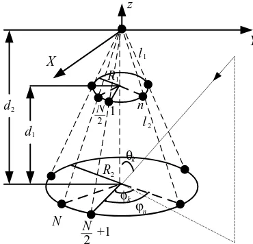
K narrowband completely polarized electromagnetic plane wave source signals from far-field impinge upon a CCCP array, which is composed ofN identical CLD pairs, as shown in Figure 1. For the CLD pairs, the dipoles parallel to thez-axis are referred to as thez-axis dipoles and the loops parallel to the
x-y plane as the x-y plane loops, respectively measuring the z-axis electric field components and the
z-axis magnetic field components. The CLD pairs’ steering vector of the kth (1≤k≤K) unit-power electromagnetic source signal is the following 2×1 vector [4, 26]:
a(θk, γk, ηk) =
ekz
hkz
=
−sinθksinγkejηk sinθkcosγk
(1)
where θk ∈ [0, π] is the signal’s elevation angle measured from the positive z-axis, γk ∈ [0, π/2] the auxiliary polarization angle, andηk ∈[−π, π] the polarization phase difference. The z-axis electric field
ekzandz-axis magnetic fieldhkzboth involve the same factor, so polarization estimation based on CLD
N
+1 2
N
n
k n 2
N 1
2
d
1
d
z
X
Y
k
1
l
2
l
1
R
2
R θ
ϕ φ
pairs is independent of the source’s direction-of-arrival, and it requires no prior information of azimuth and elevation angles.
Without loss of generality, we assume that the reference element is placed at the conical tip (origin). The distances between the reference element and the upper circular ring elements are equal to l1
(l1 ≤0.5λmin), and the distances between the reference element and the lower circular ring elements are
equal tol2 (l2 0.5λmin) where λmin is the minimal signals’ wavelength of the incident signals. On the
upper circular ring, there are N/2 elements, which have the same angle position as that on the lower circular ring. Then the data collected by the CCCP array at time tcan be represented as
X(t) =
A 1 A2
S(t) +N(t) =AS(t) +N(t) (2)
whereX(t) is the received signal, Athe (2N+ 2)×K steering vector matrix ofK incident signals,S(t) the incident signal, and N(t) the noise. A1 and A2 are sub-array steering vectors of N + 1 loops and N + 1 dipoles, respectively, which can be expressed as
A1= ⎡ ⎢ ⎢ ⎢ ⎣
sinθ1cosγ1⊗q(θ1, φ1)
sinθ2cosγ2⊗q(θ2, φ2)
.. .
sinθKcosγK⊗q(θK, φK)
⎤ ⎥ ⎥ ⎥ ⎦ T (3)
A2= ⎡ ⎢ ⎢ ⎢ ⎣
−sinθ1sinγ1ejη1 ⊗q(θ1, φ1) −sinθ2sinγ2ejη2 ⊗q(θ2, φ2)
.. .
−sinθKsinγKejηK ⊗q(θK, φK)
⎤ ⎥ ⎥ ⎥ ⎦ T (4)
q(θk, φk) =
1,qTu (θk, φk),qTd (θk, φk)
(5)
where q(θk, φk) is the spatial steering vector of whole CCCP array, qu(θk, φk) and qd(θk, φk) are respectively that of the upper and lower circular ring sub-array.
qu(θk, φk) =
⎡ ⎢ ⎢ ⎢ ⎢ ⎢ ⎣ ej
2πR1
sin(θk) cos(φk−ϕ1)−d2R−d1
1 cosθk
λ
.. .
ej
2πR1
sinθkcos
φk−ϕ N 2
−d2R−d1
1 cosθk λ ⎤ ⎥ ⎥ ⎥ ⎥ ⎥ ⎦ (6)
qd(θk, φk) =
⎡ ⎢ ⎢ ⎢ ⎢ ⎢ ⎢ ⎢ ⎢ ⎢ ⎣ ej
2πR2
sin(θk) cos
φk−ϕ N 2 +1
−d2 R2cosθk
λ
ej
2πR2
sin(θk) cos
φk−ϕ N 2 +2
−Rd2
2cosθk
λ
.. .
ej
2πR2
sin(θk) cos(φk−ϕN)−Rd2
2cosθk λ ⎤ ⎥ ⎥ ⎥ ⎥ ⎥ ⎥ ⎥ ⎥ ⎥ ⎦ (7)
with ϕn = 4π(n−1)/N n = 1, . . . , N are the angular position of array elements, and φk denotes signal’s azimuth angle measured from positive x-axis. The general assumption is that A1 and A2 are full-rank matrices. The covariance matrixRx is given by
Rx=ARsAH+σ2I (8)
eigenvectors of Rx. According to the subspace theory, the signal subspace can be expressed explicitly as
Es=AT=
A1 A2
T (9)
Es1=A1T (10)
Es2=A2T=A1ΦT (11)
whereΦ= diag([−tanγ1ejη1, . . . , −tanγKejηK]) polarization parameters can be got fromΦ
γk= tan−1(|Φkk|)
ηk= arg (−Φkk) (12) Since bothE1 and E2 are full-rank, there exists a unique nonsingular matrixΩsuch that
Es1Ω=Es2⇒Ω=
EH s1Es1
−1 EH
s1Es2 (13)
ΩT−1=T−1Φ (14)
Equation (14) implies that Φ is a diagonal matrix whose diagonal elements are composed of the
K eigenvalues of space-polarization matrix Ω, and the full-rank matrix T−1 is composed of the K
eigenvectors of matrixΩ. Then,A1 can be calculated by
A1=Es1T−1 A2=Es2T−1 (15)
The space steering vector estimates of upper circular ring is given:
˜ quθ˜
k,φ˜k
=
ˆ
A12 : N2 + 1, k ˆ
A1(1, k)
=
ˆ
A22 : N2 + 1, k ˆ
A2(1, k)
(16)
Equation (16) can be represented as follows:
˜ quθ˜
k,φ˜k
= ⎡ ⎢ ⎢ ⎢ ⎢ ⎢ ⎣ ej
2πR1
sin ˜θkcos(φk˜ −ϕ1)−d2R−d1
1 cos ˜θk
λ
.. .
ej
2πR1
sin ˜θkcos
˜ φk−ϕ N
2
−d2R−d1
1 cos ˜θk λ ⎤ ⎥ ⎥ ⎥ ⎥ ⎥ ⎦ (17)
According to Formula (17), the following relationship can be obtained:
Φ1 = arg
˜ quθ˜
k,φ˜k
= ⎡ ⎢ ⎢ ⎢ ⎢ ⎣
2πR1
sin ˜θkcos(φ˜k−ϕ1)−d2R−1d1cos ˜θk
λ ..
.
2πR1
sin ˜θkcos
˜
φk−ϕN 2
−d2−d1
R1 cos ˜θk
λ ⎤ ⎥ ⎥ ⎥ ⎥ ⎦ (18)
The space steering vector estimates of lower circular ring is given:
ˆ qdθˆ
k,φˆk
=
ˆ A1
N
2+2 :N+1, k
ˆ A1(1, k)
=
ˆ A2
N
2+2 :N+ 1, k
ˆ A2(1, k)
= ⎡ ⎢ ⎢ ⎢ ⎢ ⎢ ⎣ ej
2πR2
sin ˆθkcos(φkˆ −ϕ1)−Rd2
2cos ˆθk
λ
.. .
ej
2πR2
sin ˆθkcos
ˆ φk−ϕ N
2
−Rd2
2cos ˆθk λ ⎤ ⎥ ⎥ ⎥ ⎥ ⎥ ⎦ (19)
According to Φ1, the rough phase estimation of ˆqd(ˆθk,φˆk) is got:
Φ2 =Φ1l2 l1
(20)
The phase ambiguity number vector meets:
m(n, k) = argmin
arg
ˆ qdθˆ
k,φˆk
+ 2πm(n, k)−Φ2
From the valuem(n, k) in (21), the accurate phase vector estimation of qˆd(ˆθk,φˆk) is obtained:
D= arg
ˆ qdθˆ
k,φˆk
+ 2πm(n, k) (22)
From Formulas (19) and (22), the accurate estimation of Poynting vector is achieved:
ˆ Pkθˆ
k,φˆk
=
⎡ ⎢ ⎣
sin ˆθkcos ˆφk sin ˆθksin ˆφk
cos ˆθk
⎤ ⎥
⎦=C#D (23)
whereCis a matrix varying with elements’ position of lower circular ring, with
C= 2πR2
λ ⎡ ⎢ ⎢ ⎢ ⎢ ⎢ ⎢ ⎢ ⎢ ⎢ ⎣
1 0 −δd2
R2 cos 4π N sin 4π N
−d2 R2 .. . ... ... cos 4π N N
2 −1
sin 4π N N
2 −1
−d2
R2 ⎤ ⎥ ⎥ ⎥ ⎥ ⎥ ⎥ ⎥ ⎥ ⎥ ⎦ (24)
From Formula (23), the accurate estimates are given:
ˆ
θk= arcos
ˆ Pkθˆ
k,φˆk
3 (25) ⎧ ⎪ ⎪ ⎪ ⎪ ⎪ ⎪ ⎪ ⎪ ⎨ ⎪ ⎪ ⎪ ⎪ ⎪ ⎪ ⎪ ⎪ ⎩ ˆ
φk= arctan
⎛ ⎝
ˆ Pkθˆ
k,φˆk
2
ˆ Pkθˆ
k,φˆk
1 ⎞
⎠, Pˆkθˆ k,φˆk
1≥0
ˆ
φk=π+ arctan
⎛ ⎝
ˆ Pkθˆ
k,φˆk
2
ˆ Pkθˆ
k,φˆk
1 ⎞ ⎠, Pˆ
k
ˆ
θk,φˆk
1<0
(26)
where [·]i (i= 1,2,3) refers to the ith element in the bracketed vector. The formula involves factor cosθ, which does not introduce an ambiguity inθ, because the θin the upper hemisphere and the θ in the lower hemisphere give different cosθ.
20 30 40 50 60 70 80
Elevation (deg) 40 50 60 70 80 90 Azimuth (deg)
Figure 2. DOA scatter diagram using UCA
method.
20 30 40 50 60 70 80
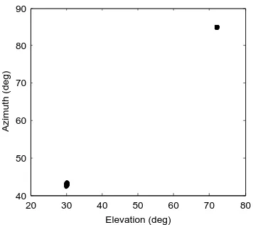
40 50 60 70 80 90 Elevation (deg) Azimuth (deg)
Figure 3. DOA scatter diagram using CCCP
20 30 40 50 60 70 70
80 90 100 110 120 130
APA (deg)
PPD (deg)
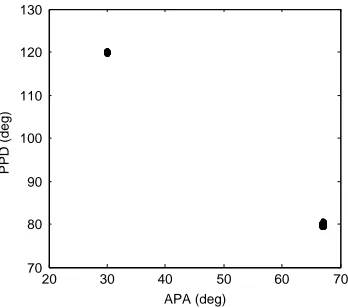
Figure 4. Polarization scatter diagram with UCA method.
20 30 40 50 60 70
APA (deg) 70
80 90 100 110 120 130
PPD (deg)
Figure 5. Polarization scatter diagram with CCCP method.
3. NUMERICAL EXAMPLES
To test the effectiveness of the proposed method, the following condition is considered. Two high-frequency incoherent sources impinge respectively on three arrays, viz., UCCA, CCCP and UCA, and there are 16 sensors on each circular ring of the three arrays above mentioned. UCCA has the same radius as CCCP whose inner circular ring radius R1 = 0.3λ and outer circular ring radius R2 = 1.5λ. UCA
with radiusR= 0.3λ. Two incident signals are taken to have bearing parameters: [θ1, φ1] = [30◦,43◦],
[γ1, η1] = [67◦,80◦], [θ2, φ2] = [72◦,85◦][γ2, η2] = [30◦,120◦], 512 snapshots per experiment, 100
independent experiments per data point.
In the first experiment, we consider a scenario with 100 independent Monte Carlo trials running on the corresponding CCCP array. The the signal-to-noise ratio (SNR) is set to 10 dB. The sets of values of the DOA and polarization variables have been represented in scatter diagrams (Figures 2–5).
From Figure 3, it is shown that almost all estimated values are located in the vicinity of actual values [θ1, φ1] = [30◦,43◦] and [θ2, φ2] = [72◦,85◦] by using CCCP method. The estimated values of [ˆθ1,φˆ1] are
in the numerical range (29.8◦,30.2◦) and (42.7◦,43.3◦). On the contrary, from Figure 2, the estimated values [ˆθ1,φˆ1] using UCA method are distributed in the range of (29.3◦,30.9◦) and (42.2◦,44.2◦). The
estimated error using UCA method is much larger than that of CCCP method.
From Figure 5, it is shown that almost all estimated values are located in the vicinity of actual values [γ1, η1] = [67◦,80◦] and [γ2, η2] = [30◦,120◦] by using CCCP method. The estimated values of ˆγ2
and ˆη2are in the numerical range (29.9◦,30.1◦) and (119.9◦, 120.2◦), respectively. On the contrary, from
Figure 4, the estimated values are distributed in the range of ˆγ2 (29.8◦,30.2◦) and ˆη2 (119.4◦,120.6◦).
The estimated error using UCA method is larger than that of CCCP method.
In the second experiment, we compare the performance of CCCP method to UCA method and UCCA method with respect to SNR. The comparison of CRLB and the above algorithms are also given. In the simulations, the SNR is from−6 to 20 dB, and 512 snapshots are used in each of the 100 independent Monte Carlo simulation experiments. The performance of standard deviation is illustrated, and the corresponding results are shown in Figures 6–9.
The solid curves with star, triangle, circular and diamond data points in Figures 6–9 respectively plot the DOA and polarization angles’ estimation standard deviation, respectively estimated by the proposed UCA, UCCA, CCCP and CRLB method, at various signal-to-noise ratio (SNR) levels. It is obviously indicated that our proposed method can work well. The performance of the proposed CCCP method is close to that of the CRLB. The proposed CCCP procedure is better than UCA and nearly the same as UCCA. Moreover, CCCP estimating elevation angle by cosθdoes not introduce ambiguity inθ, but UCCA estimating elevation angle by sinθ may introduce ambiguity inθ because the θin the upper hemisphere and the θ in the lower hemisphere give the same sinθ. The estimation precision at
-5 0 5 10 15 20 10-3
10-2 10-1 100 101
SNR (dB)
Standard Deviation of the Azimuth (deg)
CCCP Method
UCA Method
UCCA Method
CRLB
Figure 6. Standard deviation of the azimuth versus SNR.
-5 0 5 10 15 20
10-2 10-1 100 101
SNR (dB)
Standard Deviation of the Elevation (deg)
CCCP Method
UCA Method
UCCA Method
CRLB
Figure 7. Standard deviation of the elevation versus SNR.
-5 0 5 10 15 20
10-2 10-1 100 101
SNR (dB)
Standard Deviation of the APA (deg)
CCCP Method
UCA Method
UCCA Method
CRLB
Figure 8. Standard deviation of the APA versus SNR.
-5 0 5 10 15 20
10-2 10-1 100 101
SNR (dB)
Standard Deviation of the PPD (deg)
CCCP Method
UCA Method UCCA Method
CRLB
Figure 9. Standard deviation of the PPD versus SNR.
0 5 10 15
0 0.2 0.4 0.6 0.8 1
SNR (dB)
Probability of success of DOA
method of UCA method of CCCP
method of UCCA
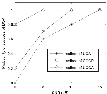
Figure 10. Probability of success of DOA versus SNR.
0 5 10 15
0 0.2 0.4 0.6 0.8 1
SNR (dB)
Probability of success of polarization
method of UCCA
method of UCA
method of CCCP
angle, 0.2◦ for auxiliary polarization angle (APA), 0.5◦ for polarization phase difference (PPD) angle, compared with that of the UCA method. The enhanced performance is rooted in the sparse embattle of CCCP. When there is no elevation quadrant ambiguity, UCCA can achieve nearly the same estimation precision as CCCP.
In the last experiment, we consider the probability of success of DOA and polarization estimations.
Here we keep the settings unchanged and set the relationship
!
(θ−θ)2+ (φ−φ)2 < 1◦ to be the
successful DOA experiment, where θ and φ denote the true DOA value and θ and φ represent the corresponding estimated value. The definition of the successful polarization experiment is the same as that of the successful DOA experiment. The result is shown in Figures 10–11.
The curves with star and circular data points in Figures 10–11 respectively plot the probability of success of DOA and polarization, respectively estimated by the UCA, UCCA and the proposed CCCP method, at various signal-to-noise ratio (SNR) levels. The proposed CCCP procedure is better and more robust than the UCA and nearly the same as UCCA procedure.
4. CONCLUSION
A new DOA and polarization estimation method based on CCCP array is proposed, which overcomes the weakness of phase ambiguity of sparse array according to short and long baselines theory. Poynting vector is obtained by the least square method, so the proposed CCCP method overcomes quadrant ambiguity in elevation angle when conical conformal array is used for wide range elevation angle (more than 90 degrees) estimation. In contrast to UCCA, CCCP does not increase computation but eliminates elevation angle quadrant ambiguity and shows better performance than UCA. CCCP has broad application prospects in airborne, missile-borne and other aerospacecrafts.
ACKNOWLEDGMENT
This work was supported by the National Natural Science Foundation of China (61201295, 61475094, 61271300). The authors would like to thank the anonymous reviewers and the associated editor for their valuable comments and suggestions that improved the clarity of this manuscript.
REFERENCES
1. Nehorai, A. and E. Paldi, “Vector sensor array processing for electromagnetic source localization,”
IEEE Trans. Signal Process., Vol. 42, No. 2, 376–398, 1994.
2. Nehorai, A. and E. Paldi, “Vector-sensor array processing for electromagnetic source localization,”
25th Asilomar Conf. Signals, Syst., Comput., 566–572, Pacific Grove, CA, 1991.
3. Wang, L. M., Z. H. Chen, and G. B. Wang, “Direction finding and positioning algorithm with COLD-ULA based on quaternion theory,” Journal of Communications, Vol. 9, No. 10, 778–784, Oct. 2014.
4. Li, J., “Direction and polarization estimation using arrays with small loops and short dipoles,”
IEEE Trans. Antennas Propag., Vol. 41, No. 3, 379–387, 1993.
5. Wong, K. T. and M. D. Zoltowski, “Polarization diversity and extended aperture spatial diversity to mitigate fading-channel effects with a sparse array of electric dipoles or magnetic loops,” IEEE Int. Veh. Technol. Conf., 1163–1167, 1997.
6. Wong, K. T. and M. D. Zoltowski, “High accuracy 2D angle estimation with extended aperture vector sensor arrays,” Proc. IEEE. Int. Conf. Acoust., Speech, Signal Process., Vol. 5, 2789–2792, Atlanta, GA, May 1996.
8. Wang, L. M., L Yang, G. B. Wang, Z. H. Chen, and M. G. Zou, “Uni-Vector-sensor dimensionality reduction MUSIC algorithm for DOA and polarization estimation,” Math. Probl. Eng., Vol. 2014, Article ID 682472, 9 Pages, 2014.
9. Li, J. and R. T. Compton, Jr., “Two-dimensional angle and polarization estimation using the ESPRIT algorithm,” IEEE Trans. Antennas Propag., Vol. 40, No. 5, 550–555, May 1992.
10. Wang, L. M., M. G. Zou, G. B. Wang, and Z. H. Chen, “Direction finding and information detection algorithm with an L-shaped CCD array,”IETE Technical Review, Vol. 32, No. 2, 114–122, 2015. 11. Li, J. and R. T. Compton, Jr., “Angle estimation using a polarization sensitive array,”IEEE Trans.
Antennas Propag., Vol. 39, No. 10, 1539–1543, Oct. 1991.
12. Yuan, X., K. T. Wong, and K. Agrawal, “Polarization estimation with a dipole pair, a dipole-loop pair, or a dipole-loop-dipole-loop pair of various orientations,”IEEE Trans. Antennas Propag., Vol. 60, No. 5, 2442–2452, May 2012.
13. Wong, K. T. and A. K. Y. Lai, “Inexpensive upgrade of base-station dumb-antennas by two magnetic loops for “blind’ adaptive downlink beamforming,”IEEE Antennas Propag. Mag., Vol. 47, No. 1, 189–193, Feb. 2005.
14. Wong, K. T., “Direction finding/polarization estimation — Dipole and/or loop triad(s),” IEEE Trans. Aerosp. Electron. Syst., Vol. 37, No. 2, 679–684, Apr. 2001.
15. Yuan, X., “Quad compositions of collocated dipoles and loops: For direction finding and polarization estimation,” IEEE Antennas and Wireless Propagation Letters, Vol. 11, 1044–1047, Aug. 2012.
16. Li, Y. and J. Q. Zhang, “An enumerative nonLinear programming approach to direction finding with a general spatially spread electromagnetic vector sensor array,” Signal Processing, Vol. 2013, No. 93, 856–865, 2013.
17. Gong, X. F., K. Wang, Q. H. Lin, Z. W. Liu, and Y. G. Xu, “Simultaneous source localization and polarization estimation via non-orthogonal joint diagonalization with vector-sensors,”Sensors, Vol. 2012, No. 12, 3394–3417, 2012.
18. Josefsson, L. and P. Persson, “Conformal array antenna theory and design,” Series on Electromagnetic Wave Theory, Wiley, IEEE Press, New York, 2006.
19. Balanis, C. A.,Antenna Theory: Analysis and Design, Wiley, New York, 2005.
20. Hansen, R. C., P. T. Bargeliotes, J. Boersma, Z. W. Chang, K. E. Golden, A. Hessel, W. H. Kummer, R. Mather, H. E. Mueller, and D. C. Pridmore-Brown,Conformal Antenna Array
Design Handbook, Department of the Navy, Air Systems Command, PN, 1981.
21. Wong, K. T. and M. D. Zoltowski, “Direction finding with sparse rectangular dual-size spatial invariance array,”IEEE Trans. Aerosp. Electron. Syst., Vol. 34, No. 4, 1320–1327, Oct. 1998. 22. Zoltowski, M. D. and K. T. Wong, “Closed-form eigenstructure-based direction finding using
arbitrary but identical subarrays on a sparse uniform cartesian array grid,” IEEE Trans. Signal Process., Vol. 48, No. 8, 2205–2210, Aug. 2000.
23. Mathews, C. P. and M. D. Zoltowski, “Eigenstructure techniques for 2-D angle estimation with uniform circular array,” IEEE Trans. Signal Process., Vol. 42, No. 9, 2395–2407, Sep. 1994. 24. Akkar, S., F. Harabi, and A. Gharsallah, “Concentric circular array for directions of arrival
estimation of coherent sources with MUSIC algorithm,”XIth International Workshop on Symbolic
and Numerical Methods, Modeling and Applications to Circuit Design, 1–5, Gammath, Italy,
Oct. 2010.
25. Wang, L. M., G. B. Wang, and Z. H. Chen, “Joint DOA-polarization estimation based on uniform concentric circular array,” Journal of Electromagnetic Waves and Applications, Vol. 27, No. 13, 1702–1714, 2013.