Optical Theorem for Transmission Lines
Edwin A. Marengo* and Jing Tu
Abstract—We present the application to transmission line systems of a new theory of the optical theorem that describes the energy budget of electromagnetic scattering in lossless wave propagation media. The insight gained by exploring this, simplest of the electromagnetic wave propagation systems from the point of view of the optical theorem, is important for understanding power budget of electromagnetic scattering due to the presence of targets in a medium, and of changes of loads due to parasitics, faults, switching, and other reasons, in transmission lines, with applications to quality control in manufacturing, self-monitoring of microwave circuits, and the detection of load changes and faults in power transmission and distribution systems. The results also apply to more general electromagnetic propagation systems and are relevant for the development of novel electromagnetic (e.g., microwave, terahertz) and optical sensors.
1. INTRODUCTION
We consider the analysis of one-dimensional electromagnetic wave propagation and scattering systems by means of the optical theorem of electromagnetics. The optical theorem is a well-known result that describes energy conservation in electromagnetic scattering phenomena [1, Secs. 13.3 and 13.6]. The form of this theorem for homogeneous plane wave excitation and free space background media is well known [1, Secs. 13.3 and 13.6]. In particular, for a scattering potential to the scalar Helmholtz partial differential operator in free space, where the scattering potential or object is interrogated by a time-harmonic homogeneous plane wave, this result states that the rate at which energy is extinct due to scattering, and absorption at the scatterer is proportional to the imaginary part of the forward scattering amplitude, corresponding to the direction of propagation of the incident plane wave [1, Page 720], [2, Eq. (1.80)]. The electromagnetic counterpart is very similar [1, Page 732]. Recently, the theorem has been successfully generalized to arbitrary fields and media, including both reciprocal and nonreciprocal lossless background media [3].
For reciprocal media [4, Page 705] it is possible to combine optical theorem principles with time reversal concepts [5, 6] applicable to reciprocal media to devise new sensors to measure real and reactive electromagnetic power extinction originating from scattering phenomena or detect the presence of targets or changes to the local propagation environment [3, Sec. VI], [7, 8]. The idea of blending the optical theorem and time reversal to design new sensors appears promising and deserves further inquiry. In this contribution we consider this topic in the context of the simplest wave propagation system, in particular, a transmission line ended by a load. This simple system is relevant on its own as well as a model for a broad range of electromagnetic wave propagation and scattering systems that can be modeled as one-dimensional, transmission-line-like systems. Such systems are relevant to microwave circuits, power transmission and distribution lines, simplified models of radar, sonar, and lidar, subsurface sensing of stratified media, and other applications. Of particular interest is the application of detecting changes to the transmission line system, such as load additions or changes (faults), via the active probing of the transmission line system and the use of the optical theorem to interpret the data. The derived
Received 9 September 2014, Accepted 15 November 2014, Scheduled 5 December 2014
* Corresponding author: Edwin A. Marengo ([email protected]).
developments are relevant to applications such as active nondestructive monitoring of faults in microwave circuits and electric power systems. The obtained results reveal previously unknown connections between the optical theorem predictions and standard results in transmission line theory, which enhances understanding of both the optical theorem and its application to transmission line problems. Furthermore, since many electromagnetic propagation systems are analogous to a transmission line, the derived results have broad applicability in novel electromagnetic and optical change detectors.
The paper is organized as follows. Section 2 reviews the basic transmission line relations. Section 3 discusses scattering in transmission line systems. Section 4 develops the main results of the paper concerning the optical theorem for transmission lines, including practical implications and corollaries of the optical theorem pertinent to transmission line systems. Section 5 illustrates the derived theory with numerical examples. Section 6 provides concluding remarks.
2. REVIEW OF THE TRANSMISSION LINE RELATIONS
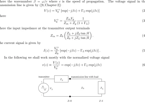
In this section we consider the baseline system in Figure 1, without the perturbations or changes whose consideration is left for the following sections of this paper. In the following, the frequency dependence is omitted with the understanding that the results hold for harmonic time dependence at a given angular oscillation frequencyω. We assume that the transmission line has lengthland real-valued characteristic impedance Z0. The transmitter’s voltage phasor and impedance are Vg and Zg, respectively. This
baseline transmission line system is ended by a passive, lossless, purely reactive load having impedance
ZL=jXL whereXL is the load reactance. The reflection coefficient atz= 0 is given by
ΓL=
ZL−Z0 ZL+Z0
exp(−2jβl) (1)
where the wavenumber β = ω/c where c is the speed of propagation. The voltage signal in the transmission line is given by ([9, Chapter 2])
V(z) =V0+[exp(−jβz) + ΓLexp(jβz)] (2)
where
V0+=
ZinVg Zin+Zg
1
(1 + ΓL) (3)
where the input impedance at the transmitter output terminals
Zin=Z0
ZL+jZ0tanβl Z0+jZLtanβl
. (4)
The current signal is given by
I(z) = V
+ 0
Z0 [exp(−jβz)−ΓLexp(jβz)]. (5)
In the following we shall work mostly with the normalized voltage signal
v(z)≡ V(z)
V0+
= exp(−jβz) + ΓLexp(jβz) (6)
Vg Zg
ZL
Z=0 Z =l
transmission line with load transmitter
Z0
+
-
which is equivalent to settingV0+= 1. The time-average power of the incident and reflected waves, Pavi
and Pavr, respectively, are given by ([9, Chapter 2])
Pavi =
1 2Z0
Pavr =−|ΓL| 2
2Z0
(7)
so that the net average power flowing into the load is
Pav =Pavi +Pavr =
1− |ΓL|2
2Z0 . (8)
3. THE SCATTERED SIGNAL
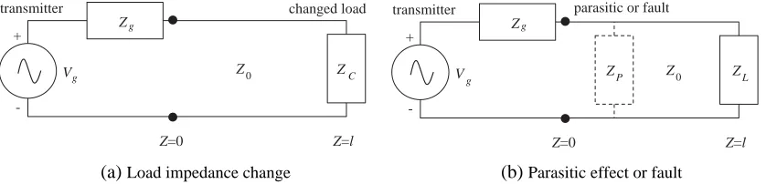
We consider next the scenario in which the transmission line system changes, e.g., due to thermal changes, spurious or parasitic loads, or as part of switching operations in the subsystem modelled as a load above, e.g., for communications, signal processing, etc. Figure 2 illustrates two scenarios of interest. Without loss of generality (since the location of the fault or change can be absorbed into the definition of the load terminals) in the following we focus on the case in Figure 2(a) with the understanding that the discussed results apply rather broadly. The load is passive and has rather arbitrary impedanceZC.
For simple notation, here and henceforth we use a caret ˆ over a quantity to denote the value of the quantity if the load changes to ZC, e.g., we denote the normalized baseline voltage signal (for ZL) as v(z) and denote the normalized voltage under a load changeZL→ZC as ˆv(z).
Borrowing from the results of the previous section we have
ˆ
v(z) = exp(−jβz) + ΓCexp(jβz) (9) where
ΓC = ΓCexp(−2jβl) (10)
where
ΓC = (ZC −Z0)
(ZC +Z0). (11)
For the baseline system the normalized reflected signal is, according to (6), equal to
vr(z) = ΓLexp(jβz) (12)
while for the perturbed system it is, according to (9), given by
ˆ
vr(z) = ΓCexp(jβz). (13)
The normalized scattered voltage signal is the difference between the baseline and perturbed reflected signals, thus from (12), (13)
v(s)(z) = ˆvr(z)−vr(z) = (ΓC −ΓL) exp(jβz). (14)
Vg Zg
ZC
Z=0 Z=l
changed load transmitter
Z0
+
-Vg Zg
ZL
Z=0 Z=l
transmitter
Z0
+
-ZP
parasitic or fault
(a) Load impedance change (b) Parasitic effect or fault
Figure 2. (a) Impedance change of the load circuit, modelled as a new loadZC. (b) Parasitic effect or
We assume next that the datum available for signal processing and detection is the value of the reflected signal at z = 0, the transmitter output terminals. Thus the measured reflected signal under the baseline system is
vrec(b) ≡vr(0) = ΓL (15)
and the scattering datum is
vscat ≡v(s)(0) = ΓC −ΓL. (16)
4. OPTICAL THEOREM APPLIED TO TRANSMISSION LINE SCATTERING
We apply next the optical theorem of electromagnetics to the study of wave scattering resulting from perturbations or changes to the original transmission line and its load. The key results are borrowed from [3] and are summarized in Appendix A.
Consider a background medium for wave propagation such as the transmission line with reactive load shown in Figure 1. Assume that a transmitter and a receiver are used to periodically probe the baseline system, so as to detect the presence of spurious targets or system changes such as those illustrated in Figure 2. Importantly, in a practical application of the results to be developed in the following, neither the baseline system nor the subsequent perturbations or changes need to be known
a priori. The transmitter and receiver used to gather the data are located outside the transmission line region under investigation. We assume, in particular, that the receiver is composed of one or more probes located in the vicinity of the transmitter output terminals (z = 0), which gather the necessary signals to be able to deduce the full linear superposition of the normalized incident plus reflected voltage wave, which defines, in turn, the value of the reflection coefficient. Equivalently, we fix V0+ = 1 and
measure the reflected signal at z= 0 as established in the discussion in (15), (16). The complex conjugate (or time-reversed) version of the voltage signal in (6) is
v∗(z) = exp(jβz) + Γ∗Lexp(−jβz). (17) The excitation V0+ that physically produces this voltage signal along the line, by radiation and
propagation, is simply V0+ = Γ∗L which is the complex conjugate of the measured reflected signal
datum v(recb) in (15), and this was expected from time-reversal electromagnetics. We therefore use in the following measurement and detection steps the complex conjugate v(recb) of the measured received signal in Eq. (15) as the key filter of any newly acquired scattering data. In particular, according to the optical theorem, since the excitation V0+= Γ∗Lproduces the complex conjugate form of the total voltage wave
in the line, including both incident and reflected parts, then it follows that if this same excitation is used to filter the scattering data in (16), then the real part () of the corresponding projection must be equal to the sum of the total power scattered by the scattered wave in (14) plus the total power absorbed (as heat or power going to another system) at the changed loadZC. We verify next that this
is, in fact, the case, corroborating the optical theorem prediction, and paving the way for a marriage between signal processing (a new optical theorem matched filtering) and power monitoring in electrical and electronic systems.
According to the optical theorem Eq. (A2), if we measure the value of the scattered signalv(s) at
z= 0, that is, vscat ≡v(s)(0) (see Eq. (16)), and filter this signal as
f =v(recb)∗vscat, (18)
then the real part of this projection
(f) =(vrec(b)∗vscat)∝P(s)+P(loss) (19) whereP(s)is the time-average scattered power, corresponding to the scattered voltage signal, andP(loss)
is the power dissipated at the loadZC. Carrying out the computation in (18) with the help of (15), (16)
we get
f = Γ∗LΓC−1 (20)
so that the real part
To see how this follows from familiar transmission line results we compute the average power of the scattered signal
P(s)= |ΓC−ΓL|
2
2Z0 =
1−2(Γ∗LΓC) +|ΓC|2
2Z0 . (22)
In addition, the power dissipated at the load is given by
P(loss) = 1 2Z0
1− |ΓC|2 (23)
so that the sum
P(s)+P(loss)= 1
Z0[1− (Γ ∗
LΓC)] (24)
and this agrees with the results in (19), (20) with proportionality constant −Z0, in particular,
(f) =(v(recb)∗vscat) =−Z0[P(s)+P(loss)], (25) as desired. In arriving at this result we use V0+= 1. For general V0+ we obtain the general expression
P(s)+P(loss)=−|V
+ 0 |2
Z0 (f) =− |V0+|2
Z0 (v (b)∗
rec vscat). (26)
We let
ΓL=|ΓL|exp(jα)
ΓC =|ΓC|exp(jγ). (27)
Then
(Γ∗LΓC) =|ΓC|cos(γ−α)
(Γ∗LΓC) =|ΓC|sin(γ−α) (28)
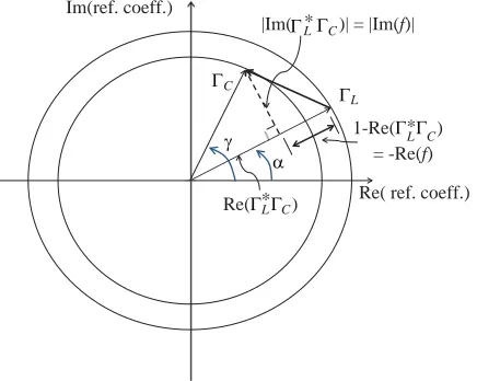
so that from (21)(f), which is a measure of the scattering real power (due to the scattered wave plus dissipation at the load), is given by
(f) =|ΓC|cos(γ −α)−1 (29)
and this has the Smith chart representation in Figure 3.
Figure 3 shows the geometric, Smith chart representation of |(f)|. According to (A3), the imaginary part(f) of f is a measure of the reactive power of the scattering phenomenon. We explain
L C
|Im( )| = |Im(f)| *
1-Re(Γ Γ * )
L C
= -Re(f) Im(ref. coeff.)
Re( ref. coeff.) ΓL ΓC
Γ
Re(Γ Γ *L C) α γ Γ
this with reference to the Smith chart as follows. For the reference reactive load the reactive power going into the load at position z is given by
PreactL (z) = 1 2(V I
∗) =|V0+|2
Z0 (ΓLexp (j2βz)) (30)
To detect changes in the reactive power it is natural to consider, as reference values for z, those for which the reactive power flowing into the load equal zero. This happens for 2βz=−α+mπ, for integer
m, where α is the phase angle of ΓL (see Eq. (27)). Since here|ΓL|= 1, this corresponds in the Smith chart to moving the original load or reflection coefficient to any of the points in the chart corresponding to reflection coefficient equal to 1 and−1. These points are in the horizontal line corresponding to zero reactance, and thus if the original load changes later to another value that has the same reactance but a different resistance, the new position of the load in the chart will remain within the same line. Thus for the changed load having reflection coefficient ΓC the reactive power at the same reference distance
is given by
PreactC (2βz =−α+mπ) = |V
+ 0 |2
Z0 |ΓC|sin(γ−α) (31)
Thus the respective change of reactive power due to the load change is given by
ΔPreact =PreactC −PreactL =
|V0+|2
Z0 (ΓCΓ ∗
L)∝ (f) (32)
as desired.
Figure 3 also shows that|f|is in fact equal to the magnitude of the scattered signal, |ΓL−ΓC|:
|f| Z0 =
|v(recb)∗vscat|
Z0 =Pap=
(P(s)+P(loss))2+ (ΔP
react)2 =|ΓC−ΓL|/Z0 (33)
wherePap denotes the scattering apparent power. Above we assumed for simplicityV0+= 1, but we can
make the results more general by adding the|V0+|2factor in some of these expressions, e.g., (33) becomes
more generally
|f||V0+|2
Z0 =
|v(recb)∗vscat||V0+|2
Z0 =Pap =
|ΓC−ΓL||V0+|2
Z0 (34)
We note from these results that the largest value of the attainable scattering apparent power is four times the probing wave power |V0+|2/(2Z0), that is 2|V0+|2/Z0, and this maximal apparent power
is in the form of pure real power carried by the scattered wave and occurs if the new load ZC is purely
reactive, and in particular, ZC = 1/ZL, as can be verified easily with reference to (39) or the Smith
chart. As an application, if the passive system represented by the load is a binary communication system (e.g., a backscattering-based RFID system), then the best choice for alternative states, representing 1 and 0, is one where 1 or 0 corresponds to a reactive load, say ZL, while the other state corresponds to
another reactive load, say ZC = 1/ZL. These alternative states maximize the magnitude of the signal |ZC −ZL| which is in fact a measure of the physical apparent power due to scattering, as we have
demonstrated above.
These general results yield some interesting special cases. Note for instance that if the change or perturbation represented by the new loadZC is purely reactive or nondissipative, then knowledge of|f|
suffices to define the magnitude of both scattering real and reactive power, in particular,
((Γ∗LΓC))2+ ((Γ∗LΓC))2= 1
((Γ∗LΓC)−1)2+ ((Γ∗LΓC))2 =|f|2
(35)
so that
(f) =(Γ∗LΓC)−1 =−|f|2/2
|(f)|=|(Γ∗LΓC)|=|f|1− |f|2/4
which in view of the discussion in (26), (32), (33) implies
P(s) = |f|
2|V+ 0 |2
2Z0
|ΔPreact|= |f|
1− |f|2/4|V+ 0 |2 Z0
Pap = |f||V
+ 0 |2 Z0
(37)
so that the magnitude of both real and reactive power associated to the load change can be deduced from the magnitude of f alone, which is very interesting and also quite relevant to high frequencies such as the optical regime in which one measures directly only field intensities. Note, however, that while the real power is positive, the reactive power can be positive or negative, and this sign remains undetermined from the knowledge of |f| alone. This implies that for nondissipative changes, all the physical power information, except only the sign of the reactive power, is carried by the magnitude of the change signal, which corresponds to the mathematical signal energy. In this special case, incoherent detection schemes such as the familiar energy detector have a real physical energy correspondence. However, the results (37) hold only for nondissipative load changes. For more general load changes, it is necessary to use the more general relations (29), (32), (34) which constitute a coherent processing scheme, in order to separately estimate the real and reactive power changes.
These results also allow us to establish, as corollaries, some bounds for the real, reactive, and apparent powers that is extinct due to the scattering, which can be used if only partial information is available about the received signal or the associated reflection coefficient. For example, if only the magnitude |ΓC| of the reflection coefficient ΓC is measured (e.g., perhaps the signal delay or phase is
unreliably captured as is the case for optical and higher frequencies) then one can still say the following about the power extinct into propagation power in the scattered wave plus dissipated power at the changed load:
(1− |ΓC|)|V0+|2
Z0 ≤P
(s)+
P(loss) ≤(1 +|ΓC|)|V + 0 |2
Z0 , (38)
and
(1− |ΓC|)|V0+|2
Z0 ≤Pap ≤
(1 +|ΓC|)|V0+|2
Z0 , (39)
as can be verified easily with reference to the geometrical interpretation in Figure 3. For generality, here we include theV0+ dependence explicitly. Also,
0≤ |ΔPreact| ≤ |
ΓC||V0+|2
Z0 . (40)
If, on the contrary, one measures phase only (as in time delay tomography), we get these bounds based on the fact that |ΓC| ≤1:
(1−cos(β−α))|V0+|2
Z0 ≤P
(s)+
P(loss) ≤ |V + 0 |2
Z0 if cos(β−α)≥0 |V0+|2
Z0 ≤P
(s)+P(loss) ≤ (1−cos(β−α))|V0+|2
Z0 if cos(β−α)≤0,
(41)
2−2 cos(β−α)|V0+|2
Z0 ≤Pap≤
|V0+|2
Z0 if cos(β−α)≥0 |V0+|2
Z0 ≤Pap≤
2−2 cos(β−α)|V0+|2
Z0 if cos(β−α)≤0,
(42)
and
0≤ |ΔPreact| ≤ |
sin(β−α)||V0+|2
5. EXAMPLES
We illustrate the preceding optical theorem developments with transmission line examples which can be used, among other applications, for communications based on the change of a load (switching) at the end of a transmission line. This is, in fact, the approach behind existing backscattering-based RFID systems. The same systems discussed in the following also simulate electromagnetic systems to detect the motion of metallic targets or changes in the surface of a material. In the latter point of view, we exploit the well-known fact that many problems of electromagnetic wave propagation are analogous to the propagation of voltage and current signals in a transmission line, with the plane wave parameters of electric and magnetic field intensity, wavenumber, and wave impedance playing the role of the transmission line parameters of voltage and current, wavenumber, and line or load impedance, respectively (see [9, Chapter 8, Table 8-1], for an overview).
Figure 4 shows the first transmission line system to be considered, which consists of a transmission line ended by a short circuit. The top part of the figure shows the (background) system corresponding to the reference signal. The possible change under consideration is the change of the position of the short circuit, by a distance δ, as shown in the bottom part of the figure. Among other applications, this can be used as a position sensor, liquid level sensor, proximity detector, and other sensors, or as a passive transmitter communication scheme (e.g., RFID) that uses probing energy from the receiver alone. Thus in a binary communication scheme, the short circuit can take two possible positions, which translate into ones and zeros that can be detected at the receiver using the optical theorem indicators developed in this work. The above transmission line system is also a simple model for an electromagnetic sensor, possibly a radar system, to sense changes in the position of a target exhibiting high electric conductivity, e.g., a person, a vehicle, machinery in an industrial facility, etc. It can thus be used to detect motion or the proximity of a target of interest.
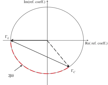
In this example the load isZL= 0 which means that the reflection coefficient at the original load
position is ΓL=−1. If the load position changes by a distanceδ, moving into the transmitter, as shown in Figure 4, then the respective equivalent reflection coefficient at the original load position is given by
ΓC = ΓLexp(j2βδ) =−exp(j2βδ). (44) This change has the Smith chart representation shown in Figure 5. The reflection coefficients (ΓL and ΓC) can be phase-shifted to their equivalent values (ΓL and ΓC) at any point in the line, say
Vg
Zg
Z0
+
-s.c. Vg
Zg
Z0
+
-s.c.
Reference load state
Equivalent load change
δ (a)
(b)
Figure 4. Transmission line system with switching load. (a) The reference load is equivalent to a short circuit at a given point in the line. (b) The changed load state is equivalent to a short circuit at a shifted position in the line.
Im(ref. coeff.)
Re( ref. coeff.)
C L
2βδ
Γ Γ
the transmitter output terminals (see (1)). However, this is not necessary for the optical theorem computations since the resulting phase shifts of ΓL and ΓC are the same, so that Γ∗LΓC = Γ∗LΓC. Thus
we can rewrite (20) as
f = Γ∗LΓC−1 (45)
which holds for any reference position used to evaluate the original load and the changed load. In the present example, we obtain from (44)
f = exp(j2βδ)−1. (46)
Assuming the normalized value V0+ = 1, it follows from (25) that the average power associated to the
scattering caused by the load change is equal to
P(s) =−(f)
Z0 = 1−cos(2βδ). (47)
It follows from (32) that the reactive power associated to the load change is
ΔPreact = (f)
Z0 = sin(2βδ). (48)
The respective apparent power is given from these results and (33) by
Pap= |f|
Z0 = √
2 [1−cos(2βδ)]1/2. (49)
Note that, as expected, the results (47), (48), and (49), for this special case involving the motion of a purely reactive load, agree with the general relations (37) applicable to an arbitrary nondissipative load change. The real, reactive, and apparent powers are periodic functions of δ, with period equal to λ/2 (where we use β = 2π/λ). The maximal value of real and apparent power occurs at δ =λ/4. This is expected from the discussion following Eq. (34), since the equivalent impedance of the short circuit at a quarter-wave distance is equal to infinity (open circuit equivalent). Thus if this system is used for a binary communication channel, the optimal choices for δ corresponding to the two possible states are
δ = 0 and δ =λ/4. Furthermore, from the discussion following Eq. (34), the same remark applies to any reactive load that could have been used in place of the short circuit, thus quarter-wave changes in the length of the transmission line segment associated to the alternating load states are optimal for binary communication purposes.
As a second example, we consider a modified version of the previous example, which is shown in Figure 6. In this case the transmission line (of impedanceZ0 and wavenumber β) is ended by a segment of length D constituted by another transmission line of impedanceZ1 that is ended by a short circuit load. The segment of transmission line has wavenumberβ1. This transmission line segment is assumed to be lossless so that bothZ1 and β1 are real-valued. This corresponds to the original condition of the system, which can change at subsequent measurements. For example, the length (D) and impedance (Z1) of the transmission line segment can change, taking possibly different values D+δ and Z1C as
illustrated in the bottom part of Figure 6. In addition, the wavenumber of the segment of transmission line can also change, from its original value of β1 to a new value of β1C. Again, for simplicity we
assume that the transmission line remains lossless so thatZ1C andβ1C are both real. The corresponding
Vg Zg
Z0
+
-
s.c. Vg
Zg
Z0
+
-
D+δ s.c.
Z1
ZC1 D
(a)
(b)
Figure 6. Transmission line concept for the second example. (a) The background system is equivalent to a segment of transmission line of impedance Z1 and length D that is ended by a short circuit load. (b) The changed system is equivalent to a transmission line segment of impedance Z1C and length D+δ that is ended
by a short circuit load.
incident wave
incident wave
reflected wave
reflected wave original dielectric slab
changed dielectric slab PEC
PEC
D+δ D
Figure 7. Electromagnetic plane wave propaga-tion analog of the system in Figure 6. Probing is done using a normally incident plane wave. The reflected wave is measured and the reflection coef-ficient is used as the key signal. The background system contains an infinite slab of dielectric ma-terial of widthDthat is bounded by a PEC wall. The possible changes that can occur to this sys-tem are shown in the bottom portion of the figure, including change of the slab width (from its origi-nal value ofDto a new value ofD+δ) or change of the constitutive properties of the dielectric ma-terial.
free space impedance η = μ0/0 where 0 and μ0 are the free space permittivity and permeability, respectively. The corresponding value of the wavenumber isβ =ω√μ00. The original slab material has permittivity and permeability1andμ1, respectively, which corresponds to impedanceη1=μ1/1and wavenumber β1 =ω√μ11. In the electromagnetic analogy, η1 corresponds toZ1. Finally, the changed
slab material has permittivity and permeability C1 and ηC1, which corresponds toη1C =
μC1/C1, and
β1C =ω
μC1C1. In the electromagnetic analogy, η1C corresponds to Z1C.
Next we present the example in the original transmission line context shown in Figure 6, with the understanding that the same results apply to the electromagnetic case in Figure 7 as well as other more general cases including oblique incidence by a plane wave, propagation in wave-guiding structures, and other situations. The reflection coefficient ΓL of the original propagation system (top part of Figure 6) evaluated at a distance D from the short circuit can be computed using well-known results (e.g., the general discussion in [10, Eq. (5-67d)]). We use a well-known result to compute the equivalent impedance of the short circuit at that point:
ZL =jZ1tan(β1D). (50)
Then the reflection coefficient at the interface of the two transmission line segments of impedance Z0
and Z1 is equal to
ΓL= jZ1tan(β1D)−Z0
jZ1tan(β1D) +Z0. (51)
line segments is equal to
ZC =jZ1Ctan[β1C(D+δ)]. (52)
The respective reflection coefficient is
ΓC = jZ
C
1 tan[β1C(D+δ)]−Z0 jZ1Ctan[β1C(D+δ)] +Z0
. (53)
Here we note that to apply our results, the reflection coefficients ΓL and ΓC must correspond to the same position in the line. We use as reference point the interface of the transmission line segments of the original, background system. We translate the reflection coefficient in (53) to this point, obtaining the corrected value
ΓC =
jZ1Ctan[β1C(D+δ)]−Z0 jZ1Ctan[β1C(D+δ)] +Z0
exp(2jβδ). (54)
Using these results and (45) we get
f = [exp(2jβδ)−1]F1−j[exp(2jβδ) + 1]F2
F1+jF2 (55)
where
F1 =z1z1Ctan (β1D) tan
β1C(D+δ)
+ 1
F2 =z1Ctan
β1C(D+δ)
−z1tan(β1D) (56)
where we have introduced the normalized impedances
z1 ≡Z1/Z0 z1C ≡Z1C/Z0.
(57)
This gives
F12+F22
(f) =F12−F22
cos(2βδ)−F12+F22
+ 2F1F2sin(2βδ)
F12+F22
(f) =F12−F22
sin(2βδ)−2F1F2cos(2βδ). (58)
It can be shown that these relations are consistent with the general results (37), as expected since the transmission line segment is nondissipative. Note that f varies periodically with 2βδ with period 2π. It also depends on F1 and F2, both of which vary periodically with β1Cδ with period 2π so that overall f varies periodically with δ with period that is smaller than or equal to the biggest between λ/2 (from the 2βδ periodicity) andλC1 = 2π/β1C (from the β1Cδ periodicity). This holds regardless of the value of D, as we illustrate with numerical results in the following.
For the special case in whichZ1C =Z1 andβ1C =β1 (the properties of the transmission line segment
remain the same) the results in (56) take the special form
F1=z12tan(β1D) tan[β1(D+δ)] + 1
F2=z1[tan [β1(D+δ)]−tan(β1D)]. (59)
Similarly, for the special case in which δ= 0 we obtain
F1 =z1z1Ctan (β1D) tan
βC1D
+ 1
F2 =zC1 tan
βC1D
−z1tan (β1D). (60)
The real, reactive, and apparent powers associated to the load change can now be evaluated by applying the general expressions (25), (32), (33) to these results. Figures 8 and 9 illustrate the dependence of the real, reactive, and apparent powers on the slab width change δ, for the special case associated to Eq. (59). In this computer illustration we adopt the following numerical values: |V0+|2/Z0 = 1 (which
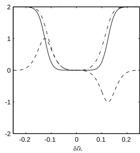
-0.2 -0.1 0 0.1 0.2 δ/λ
-2 -1 0 1 2
Figure 8. Normalized real, reactive, and apparent powers versus δ/λ for D = λ/8. Re-sults for Z1 = Z0/2 and
β1 = 2β. The solid line corre-sponds to the real power. The dashed line represents the re-active power. The dashdot line corresponds to the apparent power.
-0.2 -0.1 0 0.1 0.2
δ/λ -2
-1 0 1 2
Figure 9. Normalized real, reactive, and apparent powers versus δ/λ for D = λ/4. Re-sults for Z1 = Z0/2 and
β1 = 2β. The solid line corre-sponds to the real power. The dashed line represents the re-active power. The dashdot line corresponds to the apparent power.
-0.5 0 0.5
δ/λ -2
-1 0 1 2
Figure 10. Normalized real, reactive, and apparent powers versusδ/λ forD=λ/4. Results for Z1 = Z0/2 and β1 = β/2. The solid line corresponds to the real power. The dashed line represents the reactive power. The dashdot line corresponds to the apparent power.
example the power varies periodically withδ with periodλ/2 which indicates the detectability of spatial changes of the load associated to the half-wavelength range only. This is very interesting since in the present example, the change in question is not only a displacement of the reactive load (as in the short circuit case). Also the load itself as perceived at the interface between the two transmission line segments changes. Still, we obtain again the same detectability range, but the actual dependence on the distance in question (in the present example, the slab width changeδ) is not the sinusoidal function encountered in the short circuit case (or any other reactive load as we explained in that example). The variation depends on the background load itself as we see in these plots corresponding to two different values of
D. As another example we consider the values: |V0+|2/Z0 = 1; Z1 =Z0/2; β1 =β/2; δ ∈[−λ/4, λ/4]
where the wavelength λ= 2π/β. Figure 10 shows the variation off withδ/λforD=λ/8. In this case the power varies periodically withδ with periodλ, as expected from the discussion given after Eq. (58) since here λ1 = 2λ.
We conclude this section with a discussion of the application of the optical theorem to sensors that measure electromagnetic constitutive properties. In this context, the optical theorem provides a way to directly measure power associated to the scattering by a sample under study, which can be used to measure constitutive properties, e.g., finite conductivity giving rise to dissipated power. The use of the optical theorem is particularly relevant if the data are corrupted by noise and systematic perturbations since it involves a coherent form of signal processing which can enhance signal-to-noise ratio (SNR) in a way analogous to that of a matched filter [8]. In addition, the optical theorem can also be useful in validating model assumptions used in the interpretation and processing of sensor data, and in the analysis of limited data, since then the physical constraint of energy conservation which is at the heart of the optical theorem can be exploited to extract pending pieces of information about the sample. In this connection, we have already presented useful optical theorem corollaries which put bounds on unknown quantities (Eqs. (38)–(43)) or demonstrate dependencies that can be exploited under presumed assumptions (Eq. (37)).
Z0 Z0
short
circuit
D
sample
0 0 PEC D
transmitter
receiver
sample
(a) Transmission line system (b) Electromagnetic counterpart
δ
η η
δ
Figure 11. (a) Concept of a transmission line system to measure the constitutive properties of a material. The transmission line can be, e.g., coaxial. The transmission line segment of the sample has width δ and is placed at a distance D from a short circuit load. (b) Electromagnetic counterpart in which the sample is probed in free space with normally incident plane waves generated by a transmitter antenna and the scattered field is sensed at a receiver antenna.
general scenario in which one wishes to estimate both complex permittivity and permeability, which corresponds to 4 real parameters, requires at least 2 complex data. This can be obtained using two different reference loads, e.g., the basic short circuit and open circuit loads. In all these scenarios, reliable estimation of the sought-after properties depends, of course, on the particular sensing setup and nature of the available material samples. For example, in the system considered next the values of the parameters must obey certain model-based constraints (Eqs. (61), (62)) to ensure that the assumed signal model linking the parameters to the data remains applicable. In particular, we assume that thin samples of the material are available which can be placed as transmission line segments in the configuration in Figure 11(a) or interrogated directly in free space in the normal incidence electromagnetic counterpart in Figure 11(b). These setups are practical, see, e.g., the review in [11]. They can be implemented either as a multi-frequency sweep or using pulses and transforming to the frequency domain for processing. We discuss next the transmission line setup in Figure 11(a) with the understanding that analogous results apply to the system in Figure 11(b). We show that the open circuit load scenario, corresponding to D=λ/4 in Figure 11(a), can be used to estimate the complex permittivity of the sample material while the short circuit load scenario, corresponding to D= 0 in Figure 11(a), can be used to estimate the complex permeability of the sample material.
In measuring the complex permittivity c =−j (where includes the bound charge and the
conduction, i.e., σ/ω term, contributions), we require the sample width δ and c to be such that
ωη0|c|δ1 (61)
where η0 = μ0/0 is the wave impedance of the dielectric material between the transmission line conductors or, in the context in Figure 11(b), the free space or air surrounding the sample. In measuring the complex permeabilityμc =μ−jμ, we require δ and μc to be such that
ω|μc|δ/η0 1. (62)
These conditions ensure a desirable quasi-linear relationship between the sought-after parameters and the optical theorem quantitiesf andf which are proportional to the extinct real and reactive powers as we have established in Section 4.
In particular, it follows readily from (61), the discussion in (18), (20), and well-known transmission line relations applicable to short circuit and open circuit loads that for the open circuit load case,
D=λ/4,
(fo.c.) −2ωη0δ
(fo.c.) −2ωη0δ. (63)
Similarly, we find from (62) and basic transmission line relations that for the complementary short circuit load case, D= 0,
(fs.c.) −2ωδμ/η0
(fs.c.) −2ωδμ/η0. (64)
This means that so long as (62) holds we can measure the real and imaginary parts of the permeability directly through the optical theorem quantitiesf andf, respectively. Furthermore, we can measure useful normalized quantities that are independent of the value of the sample widthδ, which isolates the role of this nuisance parameter. Of particular interest is the estimation of the electric and magnetic loss tangents, tanδe =/ and tanδm =μ/μ, respectively, which we find from (63), (64) to be given
approximately in terms of the optical theorem quantities f and f by
tanδe (fo.c.)
(fo.c.)
tanδm (fs.c.) (fs.c.).
(65)
6. CONCLUSIONS
The optical theorem is a fundamental result in electromagnetic scattering theory. It defines the datum that carries information about the energy budget of the scattering phenomenon. This includes both real power extinction associated to dissipation and scattering as well as reactive power extinction due to energy storage around the scatterer. In this paper we have demonstrated the application of the optical theorem to the simplest of the electromagnetic wave propagation environments: the one-dimensional, transmission line system. Understanding of the optical theorem for transmission lines is fundamental for our theoretical understanding of the optical theorem, in both its classical form related to the real extinction power as well as its recently developed reactive power format [3]. This insight, in turn, paves the way for a myriad of applications in sensing and detection both of transmission line systems such as power distribution and microwave circuits as well as more complex systems that can be modelled using transmission line concepts. For instance, the optical theorem data can be used as statistics or indicators for the detection of changes in transmission-line-like systems with applications in remote sensing and communications. In this paper we rigorously validated the optical theorem predictions as they apply to transmission lines, and showed their connections to standard transmission line theory concepts such as the Smith chart. Among other results, the developed theory provided bounds for real, reactive, and apparent powers in transmission line scattering. The derived results were illustrated with numerical examples motivated by practical contexts in which optical theorem indicators can be implemented as a physically-motivated concept for sensing and change detection.
Importantly, the developed optical theorem results are applicable throughout the full electromagnetic spectrum, from the low frequency regime relevant to power transmission lines, to the high frequency range of optical and infrared fields and beyond. In the present paper we focused on the basic treatment of time-harmonic signals. We plan to address elsewhere the counterpart of the obtained results for more general, broadband signals. In addition, to remain focused, in this paper we emphasized the reflective geometry in which both transmitter and receiver probes are located at the same end of the transmission line. This case is the most relevant for the particular applications envisioned in this work. On the other hand, it is not hard to show that the same general results developed in the paper on optical theorem indicators also apply to the complementary transmissive geometry. Furthermore, one can even extend the obtained results to systems having both reflective and transmissive data. These questions provide the starting point of an interesting line of future research, with further natural extensions to the full two-dimensional and three-dimensional wave propagation systems in which we can have multiple sensors probing the scatterer as well as multiple frequency or time domain data. We plan to pursue some of these interesting research avenues in the future.
ACKNOWLEDGMENT
APPENDIX A. REVIEW OF THE GENERAL OPTICAL THEOREM RELATIONS
The key optical theorem results from [3] can be summarized as follows. Consider the active electromagnetic wave probing of a scatterer located in a region of investigation τ. The scatterer represents a change or perturbation to the given background or baseline medium which is assumed to be lossless and reciprocal. This baseline medium can be bounded or unbounded, and this is incorporated into the model via the suitable boundary conditions. The datum corresponding to a scattering experiment (m, n) is defined by 1) a known electromagnetic source (Jn (electric current
density), Mn (magnetic current density)), where n denotes the transmitter state, e.g., its position,
orientation, etc., that is located outside τ and radiates in the background medium a given incident electromagnetic field (E(ni),Hn(i)); and 2) a receiver outside τ whose output vm,n is a linear projection
of the scattered electromagnetic field (E(ns), H(ns)), onto a given state m of the electromagnetic form
(Im, Km), in particular,
vm,n =
r∈/τdr
Im·E(ns)−Km·H(ns)
. (A1)
In view of the electromagnetic reciprocity principle, Im, Km are the sources or sinks representing the
sensor or receiver, while the scattering datum vm,n has the meaning of a reaction. If these m-labeled
sources are chosen such that they radiate, in the reciprocal background medium, fields whose values within τ are (apart from a trivial multiplicative factor) equal to those of the complex conjugate fields
Em(i)∗,−Hm(i)∗ corresponding tom-labeled sources, then the datumvm,n has the simultaneous meaning of a reaction and an energy interaction, and, in particular, it carries information about the power budget of a well-defined scattering experiment which can involve one or two sources (one if m = n and two if m = n) [3]. The relation describing the power budget in question is called the generalized optical theorem. For the particular casem=nthis general result takes the following form, called the ordinary optical theorem:
1
2(vn,n) =P
(s)
n +Pn(loss) (A2)
whereis the real part,Pn(s) the total scattered power, andPn(loss)the power dissipated (as heat) inside the scatterer, upon excitation by then-labeled incident field. Furthermore, for nonmagnetic scatterers, the quantity (vn,n) corresponds to the reactive power resulting from field energy storage in the near field of the scatterer [3, Sec. V]. This reactive form of the optical theorem states that the imaginary part of vn,n is related to the net scattering reactive power exiting the region of interest minus the difference
of the magnetic and electric energies stored in the medium (withinτ) as a consequence of the scatterer or medium perturbation (in excess to what was present in the baseline system), in particular,
1
2(vn,n) =Pn,react(∂V)−2ω [difference of magn. and elec. energies] (A3) and this information can be used on top of the real-power information in (A2) as a basis for sensing and detection. For instance, the magnitude |vn,n|/2 represents the total apparent power of the scattering
phenomenon, and any of these quantities ((vn,n), (vn,n), |vn,n|) can be used as a physically
well-motivated test statistic for change detection.
REFERENCES
1. Born, M. and E. Wolf, Principles of Optics, 7th edition, Cambridge University Press, Cambridge, UK, 1999.
2. Newton, R. G.,Scattering Theory of Waves and Particles, 2nd edition, Springer-Verlag, New York, NY, USA, 1982.
3. Marengo, E. A., “A new theory of the generalized optical theorem in anisotropic media,” IEEE Transactions on Antennas and Propagation, Vol. 61, 2164–2179, Apr. 2013.
5. Fink, M., “Time reversal of ultrasonic fields. Part I: Basic principles,” IEEE Trans. Ultrason., Ferroelectrics, Freq. Control, Vol. 39, No. 5, 555–566, Sep. 1992.
6. Carminati, R., R. Pierrat, J. de Rosny, and M. Fink, “Theory of the time reversal cavity for electromagnetic fields,”Opt. Lett., Vol. 32, No. 21, 3107–3109, Nov. 2007.
7. Marengo, E. A., “Target detection based on the optical theorem,” 2013 IEEE International
Symposium on Antennas and Propagation and USNC/URSI National Radio Science Meeting, 348–
349, Orlando, Florida, Jul. 7–13, 2013.
8. Marengo, E. A. and F. K. Gruber, “Optical-theorem-based coherent scatterer detection in complex environments,” International Journal of Antennas and Propagation, Vol. 2013, Paper 231729, 12 Pages, 2013.
9. Ulaby, F. T., E. Michielssen, and U. Ravaioli, Fundamentals of Applied Electromagnetics, 6th Edition, Prentice Hall, Upper Saddle River, NJ, 2010.
10. Balanis, C. A.,Advanced Engineering Electromagnetics, John Wiley & Sons, New York, 1989. 11. Saeed, K., M. F. Shafique, M. B. Byrne, and I. C. Hunter, “Planar microwave sensors for complex