TA Spectrum

TA Spectrum

DmitriIvanov1∗_{, for the Telescope Array collaboration}

1_{University of Utah, High Energy Astrophysics Institute, Salt Lake City, Utah, USA}

Abstract.The Telescope Array (TA) experiment is measuring cosmic rays of energies from PeV to 100 EeV

and higher in the Northern hemisphere. TA has two parts: main TA and the TA low energy extension (TALE). Main TA is a hybrid detector that consists of 507 plastic scintillation counters on a 1200m - spaced square grid that are overlooked by three fluorescence detector stations. TALE is also a hybrid detector that consists of addi-tional fluorescence telescopes arranged to view higher elevations and an infill array of 103 plastic scintillation counters. In this work, we describe the combined TA surface detector (SD) and TALE fluorescence detector spectrum, check the calculation of the TA SD spectrum at the highest energies using an alternative, Constant Intensity Cut, method and discuss the declination dependence of the TA SD spectrum at the highest energies. Details of the TALE spectrum calculation have been presented in a separate work at this conference.

1 Introduction

Energy spectrum is an important tool in cosmic ray physics. Spectral features including the knee at ∼ 1015.5 _{eV, the ankle near ∼ 10}18.5 _{eV, the cutoff near} ∼ 1019.5_{eV, and, recently measured, the second knee at} ∼1017.0 _{eV and thelow energy ankleat∼ 10}16.2_{eV [3],} as well as the corresponding spectral indices, provide in-formation about the nature of the cosmic ray sources and the effects of the cosmic ray propagation. The Telescope Array (TA) is a modern cosmic ray detector, which is sen-sitive over a wide range of energies and which sees these features.

In this paper, we discuss the combined TA energy spectrum measurement, ranging from a couple of PeV to hundreds of EeV and higher, and focus on the recent devel-opments of the TA surface detector (SD) spectrum analy-sis at the highest energies: a declination dependence of the TA SD spectrum above 1019 eV, a discrepancy in the spectrum measurement between the TA and Auger experi-ments above 1019eV, and an important check of the TA SD spectrum calculation using the Constant Intensity Cut [1] analysis, which is an alternative model-independent recon-struction technique for TA. Current details of the TALE spectrum measurement and interpretation can be found in [2],[3], and [4].

2 TA Data

TA is located in the desert of Millard County, UT, USA at an altitude of∼1400m above sea level, which corresponds to∼880g/cm2 vertical mass overburden. TA is designed to measure cosmic rays using the ground array and air flu-orescence detection techniques. The main TA, which has

∗_{e-mail: [email protected]}

been in operation since 2008, consists of a surface detec-tor array of 507 plastic scintillation counters deployed on a square grid of 1200 m spacing [5], which is overlooked by 3 fluorescence detector (FD) stations [6, 7]. Each TA SD counter uses 2 layers of 3m2_{×1.2cm plastic scintillator.}

The TA low energy extension (TALE) consists of 10 additional fluorescence telescopes at the Northern TA flu-orescence detector site, called the TA Middle Drum (MD), and an infill array of 103 counters of 400 and 600 m spac-ing in front of the TA MD site. The TALE fluorescence telescopes extend the TA FD field of view from the origi-nally designed range of 3 to 33oin elevation to 57oin ele-vation. This allows a reconstruction of lower energy cos-mic rays in fluorescence and ˇCerenkov mode by the TA FD, thus extending the sensitivity of the TA experiment from the original design range of 1 EeV and higher down to a couple of PeV [3]. The TALE FD has been taking data since 2014.

3 Combined TA Spectrum

(E/eV)

10

log

15

16

17

18

19

20

]

-1

s

×

-1

sr

×

-2

m

×

2

J [ eV

×

3

E

24

10

TA Combined (2018)

Auger 2017, E rescaled by +10.2%

KASCADE-Grande (2012)

Figure 1.The combined TA spectrum (black points) presented at the UHECR-2018 conference: energy range from 1015.3_{to 10}18.3_{eV is}

covered by the TALE FD [3], while the TA SD measurement [10] starts at 1018.2_{eV and extends to 10}20_{eV and higher. Superimposed}

are the Auger combined spectrum [9], with the Auger energies rescaled by+10.2% (red squares), and the KASCADE-Grande spectrum [8] (green triangles).

band that is within the field of view of the Auger, and second, we check the TA SD spectrum calculation using the Constant Intensity Cut [1] energy reconstruction tech-nique, implemented in a way similar to that of the Pierre Auger experiment.

4 Declination Dependence of the TA SD

Spectrum

Figure 2 shows the TA SD spectrum calculated for the lower and higher declination bands, which correspond to −15.7◦ < δ < 24.8◦ and 24.8◦ < δ < 90◦, respectively. In the lower declination band,−15.7◦ < δ <24.8◦, which is visible to the Auger experiment, the cutoff energy of the TA spectrum occurs at a significantly lower energy of 1019.59+0.05

−0.07eV, which is well within 1σof the Auger result, 1019.62±0.02 _{eV [11, 12]. The global chance probability of} this effect has been evaluated using the Monte Carlo to be 3.5σ.

5 Check of the TA SD Spectrum

5.1 Standard Reconstruction

As it can be seen in [14] and [15], the standard reconstruc-tion of surface detector events in TA is done as follows. First, counter time and pulse height information are fitted

to determine the arrival direction of the event. Then, a fit of the counter pulse height information into the AGASA lateral distribution function [16] is performed, to deter-mine S800, which is the signal size 800 m from the shower axis. An initial energy estimate,EMODEL[ S800,sec(θ) ], in terms of the reconstructed S800 and zenith angle, has been derived from a detailed CORSIKA [17] Monte Carlo, that uses proton QGSJET II.3 [18] hadronic interaction model, executed with the optimal thinning approximation [19], and de-thinned [20] to restore the important information on the ground. The final energy has been rescaled to the TA fluorescence detector using well reconstructed hybrid events seen by the TA SD and the TA FD in common:E= 1/1.27×EMODEL[14]. In other words, in the case of the proton QGSJET II.3 model, the model-derived SD energy is related to the energy given by the fluorescence detector via the calibration factor 1.27: EMODEL=1.27×EFD.

(E/eV)

10

log

19 19.2 19.4 19.6 19.8 20 20.2 20.4

]

-1

s

-1

sr

-2

m

2

J [ eV

3

E

24

10

+0.03 -0.03

/eV) = 19.85

2

(E

10

log :

o

> 24.8

δ

+0.05 -0.07

/eV) = 19.59

2

(E

10

log :

o

< 24.8 δ

Figure 2. The TA SD energy spectrum in the two declination

bands [13]. Filled red circles correspond to the spectrum in the lower declination band,−15.7◦ _{< δ <}

24.8◦

, and open black circles represent the spectrum in the higher declination band, 24.8◦ _{< δ <}

90◦

. Solid lines show the broken power law fits that correspond to each declination band. The cutoffenergies (log10(E2/eV)) are 19.59+0

.05

−0.07for the lower and 19.85+ 0.03

−0.03for the

higher declination bands. The cutoffenergies in the two declina-tion bands are 4σdifferent.

extreme case is well within 10% per decade of energy. Finally, we check the non-linearity of the SD energy by directly comparing the reconstructed SD energies (using proton QGSJET II.3 model) with the FD energies using hybrid events. As Figure 4 shows, there is no evidence of a non-linearity of the SD energy with respect to the FD.

5.2 Constant Intensity Cut Method

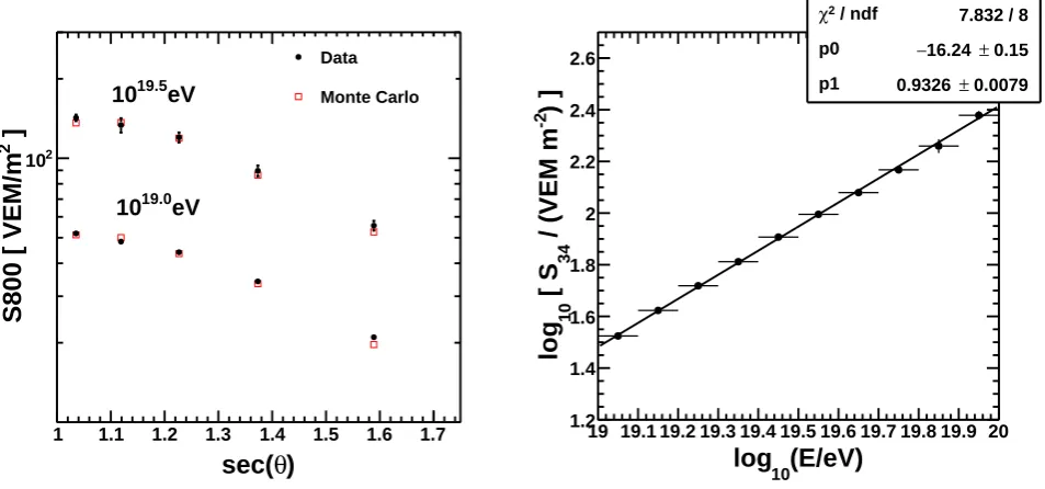
The 100% efficiency plateau of the TA SD occurs near 1019 _{eV. In the 9 years of operation, the TA SD has} ac-cumulated enough events to allow one to perform the Constant Intensity Cut (CIC) [1] analysis, which is a model-independent way of deriving the attenuation curve of the event S800 with respect to the event zenith an-gle. The left panel of Figure 5 shows the CIC curve derived from the TA SD data, and the right panel of Figure 5 shows the normalization of the energy estima-torS34 to the FD, from which we obtain the expression for the SD energy: log10(ECICSD/eV) = ([16.2 ±0.3] + log₁₀[S34/(VEM m−2)])/(0.93 ±0.02). Figure 6 shows the constant intensity cut procedure applied to the TA SD Monte Carlo. The data and Monte Carlo CIC attenua-tion curves agree, as the left panel of Figure 6 shows, and S34 versus energy relationship obtained from the TA SD Monte Carlo agrees with that obtained from the data, as it can be seen by comparing the right panels of Figures 5 and 6. Next, Figure 7 shows the comparison of the TA SD energies reconstructed using the TA SD standard

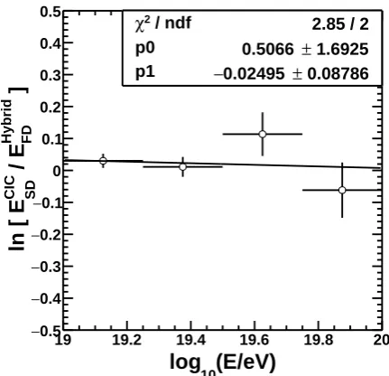
struction method described in Section 5.1 and the recon-struction using the CIC method. The two methods, as it can be seen on the right panel of Figure 7, agree at a∼3% level. Finally, as Figure 8 demonstrates by comparing the SD and FD energies of the hybrid events, the CIC method does not have an energy-dependent reconstruction bias.

5.3 Spectrum Comparison

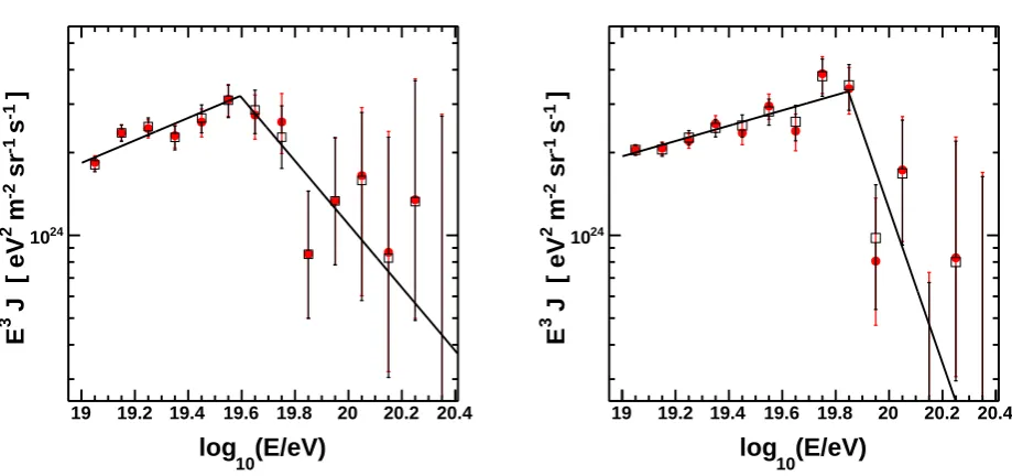
Having described and validated the two independent meth-ods of estimating the energy of the TA SD events, we can now compare the TA SD energy spectra, calculated by these two methods. Figure 9 shows the comparison of the TA SD spectra calculated using both methods in the lower (left panel) and the higher (right panel) declination bands. As it was expected from the energy comparisons of Figure 7, the spectra in Figure 9 are in excellent agreement.

6 Summary

We have provided a combined TA spectrum measurement using the most recent results of the TA SD and TALE FD. The combined TA spectrum starts at 1015.3_{eV and extends} to 1020.3 _{eV, covering 5 orders of magnitude in energy.} Cosmic ray spectrum features theknee, thelow energy an-kle, thesecond knee, theankle, and thecutoffhave all been observed in the TA data.

We have compared the combined TA spectrum to the spectra of the KASCADE-Grande and the Pierre Auger Observatory, and we have found a reasonable agreement over a wide range of energies, excluding the energies above 1019.4_{eV, where the TA and Auger full sky spectra} have a significant discrepancy. We have established that this TA and Auger discrepancy can be, in part, explained by the 3.5σ(global significance) declination dependence of the TA SD spectrum: when the Auger and TA spec-tra are restricted to the commonly seen declinations, their cutoffenergies are in a good agreement.

We have taken further steps to verify that the declina-tion dependence of the TA SD spectrum is not an instru-mental effect. In addition to the tests already performed in [13], we have re-examined the systematic uncertainties of our standard SD reconstruction by checking the linear-ity of the SD energy reconstruction with respect to the hadronic models as well as the FD in Section 5.1, and by cross-checking the results of our standard SD reconstruc-tion with the Constant Intensity Cut method in Secreconstruc-tions 5.2 and 5.3.

For a more detailed discussion on the recent Auger and TA spectrum comparisons, and the systematic un-certainties of the two experiments, an interested reader should consult the UHECR 2018 TA-Auger energy spec-trum working group report [21].

7 Acknowledgements

(E/eV) 10 log

19 19.2 19.4 19.6 19.8 20

)

FD

/E

MODEL

log(E

0.3

−

0.2

−

0.1

−

0 0.1 0.2 0.3 0.4 0.5 0.6 0.7

QGSJET-II.3 EPOS (2014) QGSJET-II.4 QGSJET-I Sybill

(E/eV) 10 log

19 19.2 19.4 19.6 19.8 20

) (normalized to FD)

FD

/E

MODEL

log(E −0.2 0.15

−

0.1

−

0.05

−

0 0.05 0.1 0.15 0.2 0.25 0.3

QGSJET-II.3 EPOS (2014) QGSJET-II.4 QGSJET-I Sybill

Figure 3. (LEFT): SD to FD calibration factors for a various hadronic interaction models (proton composition) as functions of true

(Monte Carlo) energy. Same SD to FD calibration factors after dividing out the overall constants. In the extreme case of Sybill, the energy non-linearity is within 10% per decade of energy.

p0 0.9769 ± 1.9671

p1 −0.04991 ± 0.10223

(E/eV)

10

log

19 19.2 19.4 19.6 19.8 20

]

Hybrid FD

/ E

Standard SD

ln [ E

0.5

−

0.4

−

0.3

−

0.2

−

0.1

−

0 0.1 0.2 0.3 0.4 0.5

p0 0.9769 ± 1.9671

p1 −0.04991 ± 0.10223

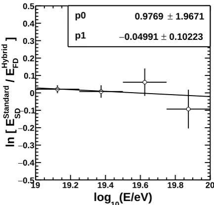
Figure 4. Natural log of the ratio of the calibrated surface

de-tector energy to the fluorescence dede-tector energy, plotted ver-sus energy. A fit to a straight line gives a slope of -0.05 that is within its fitting uncertainty of 0.10, indicating that there is no non-linearity of the SD energy with respect to the FD.

through Grants-in-Aid for Priority Area 431, for Spe-cially Promoted Research JP21000002, for Scientific Re-search (S) JP19104006, for Specially Promoted ReRe-search JP15H05693, for Scientific Research (S) JP15H05741, for Science Research (A) JP18H03705 and for Young Scien-tists (A) JPH26707011; by the joint research program of the Institute for Cosmic Ray Research (ICRR), The Uni-versity of Tokyo; by the U.S. National Science Founda-tion awards PHY-0601915, PHY-1404495, PHY-1404502, and PHY-1607727; by the National Research Foundation

)

θ

sec(

1 1.1 1.2 1.3 1.4 1.5 1.6 1.7

]

-2

S800 [ VEM m

10 20 30 40 50

/ ndf 2

χ 17.45 / 15

Constant 54.34 ± 2.138

Mean 0.8819 ± 0.05227

Sigma 0.5115 ± 0.02902 / ndf

2

χ 17.45 / 15

Constant 54.34 ± 2.138

Mean 0.8819 ± 0.05227

Sigma 0.5115 ± 0.02902

(E/eV)

10

log

18.8 19 19.2 19.4 19.6 19.8 20 20.2

) ]

-2

/ (VEM m

34

[ S

10

log

1.4 1.6 1.8 2 2.2 2.4 2.6

Entries 242 / ndf

2

χ 6.358 / 7 p0 −16.2 ± 0.3 p1 0.9307 ± 0.0162 Entries 242

/ ndf

2

χ 6.358 / 7 p0 −16.2 ± 0.3 p1 0.9307 ± 0.0162 Entries 242

/ ndf

2

χ 6.358 / 7 p0 −16.2 ± 0.3 p1 0.9307 ± 0.0162

Figure 5. (LEFT): Minimum cuts on S800 that maintain a constant number of events in the equal-intensity angular bins for the TA

SD data, plotted versus secant of the event zenith angle (θ). Solid line represents a fit to a Gaussian. Since the mean zenith angle of this data set is 34◦

, we choose to normalize the Constant Intensity Cut Curve (CIC) so that it is unity at sec(34◦

). We define

S34 =S800/CIC(sec(θ)) to be the estimator of the shower energy (E). Physically,S34represents the S800 of a shower of the same

energyEbut arriving at a zenith angle of 34◦

instead ofθ. (RIGHT): Logarithm of the energy estimatorS34plotted versus the logarithm

of the energy for well reconstructed events that have been seen by both SD and FD. Open circles show the individual hybrid events, solid circles show the mean values of log10(S34) in the log10(E) bins, and the solid line represents the linear fit.

)

θ

sec(

1 1.1 1.2 1.3 1.4 1.5 1.6 1.7

]

2

S800 [ VEM/m

2

10

Data

Monte Carlo

eV

19.5

10

eV

19.0

10

/ ndf

2

χ 7.832 / 8

p0 −16.24 ± 0.15

p1 0.9326 ± 0.0079

(E/eV)

10

log

19 19.1 19.2 19.3 19.4 19.5 19.6 19.7 19.8 19.9 20

) ]

-2

/ (VEM m

34

[ S

10

log

1.2 1.4 1.6 1.8 2 2.2 2.4 2.6

/ ndf

2

χ 7.832 / 8

p0 −16.24 ± 0.15

p1 0.9326 ± 0.0079

Figure 6. Left: The CIC attenuation comparisons between the data (black solid points) and the Monte Carlo (red open squares), for

two energy thresholds, 1019.0_{and 10}19.5_{eV. Right: The energy estimator log}

10(S34) plotted versus the logarithm of the true energy for

/ eV ]

Standard

[ (E

10

log

19 19.2 19.4 19.6 19.8 20 20.2

/ eV)

CIC

(E

10

log

19 19.2 19.4 19.6 19.8 20

20.2 Entries 3684

Mean 0.008263

RMS 0.03487

] Standard /E CIC log[E

0.2

−0 −0.15 −0.1 −0.05 0 0.05 0.1 0.15 0.2

200 400 600 800 1000 1200 1400 1600 1800 2000

Entries 3684

Mean 0.008263

RMS 0.03487

Figure 7.Event by event comparison of the TA SD standard and CIC reconstruction methods. Left panel shows the scatter plot and the

right panel shows the ratio of the energies calculated by the standard and CIC methods.

/ ndf 2

χ 2.85 / 2

p0 0.5066 ± 1.6925 p1 −0.02495 ± 0.08786

(E/eV)

10

log

19 19.2 19.4 19.6 19.8 20

]

Hybrid FD

/ E

CIC SD

ln [ E

0.5

−

0.4

−

0.3

−

0.2

−

0.1

−

0 0.1 0.2 0.3 0.4 0.5

/ ndf 2

χ 2.85 / 2

p0 0.5066 ± 1.6925 p1 −0.02495 ± 0.08786

Figure 8. Natural log of the ratio of the TA SD energy

(E/eV)

10

log

19 19.2 19.4 19.6 19.8 20 20.2 20.4

]

-1

s

-1

sr

-2

m

2

J [ eV

3

E

24

10

(E/eV)

10

log

19 19.2 19.4 19.6 19.8 20 20.2 20.4

]

-1

s

-1

sr

-2

m

2

J [ eV

3

E

24

10

Figure 9.The TA SD energy spectra calculated using the CIC method, shown as red filled circles, and the standard TA method, shown

as the open squares. The left panel compares the results for the lower declination band,−15.7◦ _{< δ <} 24.8◦

, and the right panel compares the results for the higher declination band, 24.8◦_{< δ <}

90◦ .

References

[1] J. Hersil, I. Escobar, D. Scott, G. Clark and S. Olbert, Phys. Rev. Lett.6, 22 (1961)

[2] T. AbuZayyad, C.C. Jui, et. al UHECR 2018 confer-ence

[3] R. U. Abbasiet al.[Telescope Array Collaboration], Astrophys. J. 865 (2018) no.1, 74 [arXiv:1803.01288 [astro-ph.HE]].

[4] T. Abu-Zayyad et al., arXiv:1803.07052 [astro-ph.HE].

[5] T. Abu-Zayyad et al. [Telescope Array Collab-oration], Nucl. Instrum. Meth. A 689 (2012) 87 [arXiv:1201.4964 [astro-ph.IM]].

[6] T. Abu-Zayyadet al.[Telescope Array Collaboration], Nucl. Instrum. Meth. A609(2009) 227

[7] T. Abu-Zayyadet al.[Telescope Array Collaboration], Astropart. Phys. 39-40 (2012) 109 [arXiv:1202.5141 [astro-ph.IM]].

[8] W. D. Apelet al., Astropart. Phys.36(2012) 183 [9] F. Fenu [Pierre Auger Collaboration], PoS ICRC2017

(2018) 486

[10] Y. Tsunesada, T. AbuZayyad, D. Ivanov, G. Thom-son, T. Fujii and D. Ikeda, PoS ICRC2017(2018) 535 [11] T. AbuZayyadet al., Proceedings of the 2016

Con-ference on Ultrahigh Energy Cosmic Rays, Kyoto (Japan).

[12] D. Ivanov [Telescope-Array and Pierre Auger Col-laborations], PoS ICRC2017(2018) 498

[13] D. Ivanov [Telescope Array Collaboration], PoS ICRC2017(2018) 496

[14] T. Abu-Zayyad et al. [Telescope Array Collabora-tion], Astrophys. J. 768 (2013) L1 [arXiv:1205.5067 [astro-ph.HE]]

[15] D. Ivanov, Energy Spectrum Measured by the Tele-scope Array Surface Detector, Ph.D. thesis, Rutgers— The State University of New Jersey, Department of Physics and Astronomy, Piscataway, New Jersey, USA (October 2012).

[16] K. Shinozaki et al. [AGASA Collaboration], Nucl. Phys. Proc. Suppl.136(2004) 18

[17] J. Knapp and D. Heck, Nachr. Forsch. zentr. Karl-sruhe30(1998) 27.

[18] S. Ostapchenko, Nucl. Phys. Proc. Suppl.151(2006) 143 [hep-ph/0412332].

[19] M. Kobal, Astropart. Phys.15, (2001) 259

[20] B. T. Stokes, R. Cady, D. Ivanov, J. N. Matthews and G. B. Thomson, Astropart. Phys. 35 (2012) 759 [arXiv:1104.3182 [astro-ph.IM]].