Two-dimensional quantitative visualization of isolator shock
trains by rainbow schlieren deflectometry
Atsushi Matsuyama1,*, Shinichiro Nakao1, Daisuke Ono1, Yoshiaki Miyazato1, Masashi Kashitani2
1Department of Environmental Engineering, The University of Kitakyushu, 1-1, Hibikino, Wakamatsu-ku, Kitakyushu, 808-0135, Japan 2Department of Aerospace Engineering, National Defence Academy, 1-10-20, Hashirimizu, Yokosuka, Kanagawa, 239-8686, Japan
Abstract. The rainbow schlieren deflectometry is effective in studying quantitatively the density fields in shock-containing free jets at high precision and high spatial resolution. However, there has been no practical application of rainbow schlieren deflectometry for shock trains in a confined duct. Therefore, in the present study, the rainbow schlieren deflectometry is applied to the flow field including a shock train in a constant-area duct where just upstream of the shock train the freestream Mach number is 1.34, the unit Reynolds number is 5.39 × 10⁷ m-1, and the boundary layer displacement thickness is 0.149 mm. As a result, a two-dimensional density field of the shock train is for the first time quantitatively displayed and the fine structure of the shock train is illustrated as a color gradation representation.
1 Introduction
Over the past few decades, the development of dual-mode scramjet engines for realizing next-generation propulsion systems has been aggressively conducted. Dual-mode scramjet engines provide a practical solution to supersonic flight by operating under a wide range of Mach numbers. In the ramjet mode, the incoming air is compressed through a sequence of shocks known as precombustion shocks before entering the combustion chamber. To isolate the effect of flight conditions on precombustion shocks, a nearly constant area duct referred to as an isolator is placed between the inlet and the combustor. The isolator is effective in holding the entire shocks. However, the isolator length is typically determined from empirical correlations to withstand the maximum pressure rise expected between the inlet and the exit. Being able to predict the length of a precombustion shock structure is the key component of isolator design for dual-mode scramjet engines. Also such a repeated shock structure appears in a variety of flow-devices including supersonic wind tunnels, supersonic ejectors, supersonic inlets of aircraft engines, etc and has been called in many ways by many researches, multiple shocks, shock system, for example. We refer to such a series of shocks as a "shock train". The shock train is usually followed by an adverse pressure gradient region, if the duct is long enough. The interaction region including both the shock train and the subsequent static pressure recovery region is referred to as a "pseudo-shock". However, the technical term "shock train" as well as "pseudo-shock" has been used in confusing way in most of previous articles. A review of the past experimental, theoretical, and numerical investigations on the subject of shock train and
pseudo-shock phenomena in internal gas flows is given by Matsuo et al [1].
As a result from the past investigations, it is found that a shock train occurs as a result of the interaction between a normal shock wave and a boundary layer developing along the wall surface in a confined duct. In almost all the previous experimental investigations, shock trains were studied by wall pressure measurements and schlieren optical observation. Global properties of shock trains including the pressure rise due to the shock train, the distances between each shock in a shock train, the number of shocks constituting a shock train, and the longitudinal length of a shock train are significantly influenced by three main parameters just upstream of the shock train, i.e., the freestream Mach number, the Reynolds number based upon the boundary layer characteristic thickness such as the boundary layer thickness or boundary layer momentum thickness, and the blockage ratio or the confinement levels as characterized by the ratio of the boundary layer thickness to the duct half height in case of two-dimensional duct or duct radius in case of circular duct.
Another possible measuring technique to obtain the density field of shock train is considered to be the rainbow schlieren method [3]. Howes et al. [4] devised conventional schlieren methods using the filter with continuous color gradation instead of an usual tricolour filter used in colour schlieren techniques. Kolhe et al. [5] applied the rainbow schlieren deflectometry for supersonic micro jet flow issued from a orifice, and measured the flow characteristics of the shock-containing jet qualitatively and quantitatively. Yamamoto et al. [6] measured the density fields in the correctly expanded supersonic jets issued from an axisymmetric convergent-divergent nozzle with a design Mach number of 1.6. Takano et al. [7] measured the density field of an underexpanded sonic jet by the rainbow schlieren deflectometry combined with the computed tomography. However, almost all the studies by rainbow schlieren deflectometry have been applied for free jet issued from nozzles. To the authors' knowledge, Chaganti et al. [8] was for the first time applied a rainbow schlieren deflectometry for internal shock containing flows to understand the physics of the shock-wave boundary-layer interaction. However, their rainbow schlieren technique does not have accurate enough to describe the density field of the shock wave boundary layer interaction.
Many researchers often compare simulated schlieren or shadowgraph images directly with those from experiments having the same flow conditions in order to validate the simulation. In some cases, the validation of the simulation has been performed by comparing the simulated result with the experimental wall pressure distribution in the region where the shock train occurs. However, even though simulated schlieren picture or wall pressure is in good agreement with an experimental one, a whole internal flow characteristics including the shock train cannot always be captured correctly by the computation. Until recently, very little quantitative assessments of simulations with scalar or vector properties such as the temperature, density, pressure, and velocity have been available in the flow field of shock trains. Therefore, the aims of the present study are to provide the reliable experimental data of density fields for validating a variety of numerical simulation codes on shock trains and to clarify the details of shock train structure.
2 Experimental apparatus
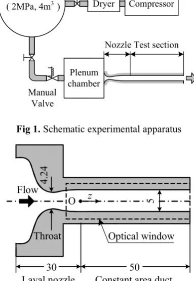
Experiments were carried out in a blow down facility with a rainbow schlieren optical system of the High-Speed Gasdynamics Research Laboratory at the University of Kitakyushu. A schematic diagram of the experimental apparatus is shown in Fig 1. The air supplied by a compressor is filtered, dried and stored in a plenum chamber and it is discharged into the atmosphere through a test section. The pressure in the plenum chamber is automatically controlled and maintained constant during the testing by a solenoid valve. The operating pressure ratio of plenum to back pressures varies from 1.5 to 2.5.
Figure 2 shows a schematic diagram of a test section. The test section consists of a supersonic nozzle followed by a constant area two-dimensional duct. The nozzle is designed by the method of characteristics to provide uniform and parallel flow at the nozzle exit plane and its design Mach number is 1.5. The nozzle has heights of 4.24 mm and 5 mm at the throat and exit, respectively, and it is a constant width of 13 mm over the full length from the inlet to exit. A two-dimensional constant area duct with a height of 5 mm and a width of 13 mm is connected to the exit of the supersonic nozzle. The dashed line in Fig. 2 indicates the range of an optical window for flow visualization by the rainbow schlieren deflectometry.
Fig 1. Schematic experimental apparatus
Fig 2. Schematic drawing of test section
3 Rainbow schlieren optical system
The present rainbow schlieren system consists of rail-mounted optical components including a 3 mm × 50 μm
rectangular pinhole, two 100 mm diameter, 500 mm focal length achromatic lenses, a computer generated 23 mm wide slide with color gradation in a 1.4 mm wide strip, and a digital camera. A continuous LED light source is connected to a 50 μm diameter optical fiber.
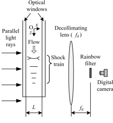
Figure 3 shows a schematic drawing of a part of the present rainbow schlieren system including the test section, the decollimating lens, rainbow filter and digital camera. The parallel light rays coming from the collimating lens are passing through the test section, refracted at the decollimating lens, and then passing through the location of the background hue on the rainbow filter at the focal
Compressor Dryer
Air Tank ( 2MPa, 4m3 )
Plenum chamber
Test section
Manual Valve
Nozzle
50 Laval nozzle30 Constant area duct
z
4.
24
5
Throat O Flow
plane of the decollimating lens before reaching the digital camera. Rainbow schlieren methods are eliminate problems associated with inhomogeneous absorption of light by the test medium and nonlinearities in recording the image.
Fig 3. Sketch of rainbow schlieren system The rainbow filter used in the present experiments is shown in Fig 4. It was fabricated in computer software and then printed digitally on a high resolution 23 mm color film recorder. It has continuous hue variation from Hue = 0 to 360 deg in a 1.4 mm wide strip. The characteristics of the rainbow filter were performed by traversing the filter in intervals of 0.05 mm in the z direction at the schlieren cut-off plane before starting experiments.
Fig 4. Rainbow filter
The calibration curve of the rainbow filter used in the present study is shown in Fig. 5 with the experimental data expressed as open symbols. The solid line indicates a least squares regression of the experimental data. As shown in Fig. 4, the background hue in the rainbow filter for the present experiment is Hue= 180 deg.
Fig 5. Calibration curve of rainbow filter
4 Method for obtaining density fields
If there is no air flow in the test section, the light rays from the collimating lens pass through the location of the background hue on the rainbow filter. On the other hand, if there is air flow with density gradients in the test section, some part of the light rays from the collimating lens is deflected when passing through the test section. The deflection angle of a light ray after passing through the test section is given by the following relation.
d
d
f
(1)where fd is the focal length of the decollimating lens and d is the ray transverse displacement from the location of the background hue. The direction at which the light ray after passing through a refracted index field in the test section is travelling are not influenced by the existence of optical windows and it remains the same regardless of whether or not there are optical windows if the windows have uniform refractive index and both the surfaces of each window are parallel to each other. In the case the light ray from the test section is passing through the same location on the rainbow filter regardless of the existence of the optical windows because the rainbow filter is positioned at the focal plane of the decollimating lens. For the schlieren picture with the vertical rainbow filter corresponding to the vertical knife edge for the conventional gray scale schlieren, density gradients in the flow direction (z axis) after passing through the test section with a width L are given by the following relation.
z
KL
(2)K = 2.26 × 10⁻⁴ m3/kg is Gladstone-Dale constant, L =13 mmis the duct width over the span direction as shown in Fig. 3. As K hardly depends on the wavelength of light, the same constant is used for all wavelengths. The Rainbow
filter Decollimating
lens ( fd )
Digital camera Parallel
light rays
Shock train
fd L
Optical windows
z x O
Flow
1.4 mm
23
m
m
360 0
d[mm] O
180 Hue [deg]
Image of background hue (Hue = 180 deg)
-0.6 -0.4 -0.2 0 0.2 0.4 0.6 0.8
0 60 120 180 240 300 360
d
[m
m
]
integration of Eq. (2) with respect to the z yields the density distribution within the shock trains.
z y, 1 z dz C y
KL
(3)where C(y) is the integral constant and it can be obtained from boundary conditions as follows. There are two boundary conditions to specify the C(y) of Eq. (3). One is the density just upstream of the shock train and the other is that at the duct exit when the exit flow is subsonic.
For the former boundary condition, the density upstream of the shock train is specified under the assumption of isentropic flow from the plenum chamber to the nozzle exit. In case of the latter boundary condition, the Mach number at the duct exit can be derived from the equation of continuity between the nozzle throat and the duct exit under the assumption that the flow is isentropic from the plenum chamber to the throat and adiabatic from the throat to the duct exit.
From the assumption described above, a relation on the exit Mach number can be derived
1 1
2 1 2 2
os
e e
b e
* 1 1 1
2 2
p A M M
p A
(4)
The equation of state at the duct exit gives e
e e p RT
(5)
where pe is equal to the back pressure pb because of subsonic flows at the duct exit and the exit temperature Te is obtained from the condition of adiabatic flow Tos = Tb through the whole flow field including the shock train and Me from Eq. (4), i.e.,
2 os e e 1 1 2 T M T
(6)
Combination of Eqs. (3) ~ (6) yields the density field within the shock train. In the present study, the density upstream of the shock train was specified as the boundary condition.
5 Results and discussion
5.1 Rainbow schlieren visualization
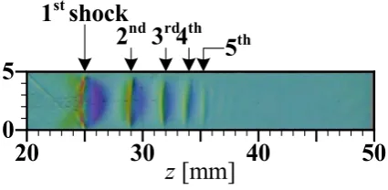
A typical rainbow schlieren picture of a shock train is presented in Fig. 6 with the flow from left to right. The picture was taken with a vertical rainbow filter to visualize the density variation in the flow direction where the plenum pressure pos is 185.6 kPa, the back pressure pb = 103.1 kPa is equal to the atmospheric pressure, and the atmospheric temperature Tb is 291.9 K.
The boundary layer thickness 1 just upstream of the shock train can be estimated from relations shown below. For compressible boundary layers on a flat-plate,
1
1 1 1
0
1 1 1
*
1
u d
u
(7)where denotes the normal distance from the duct wall normalized by 1.
Fig 6. Rainbow schlieren picture
From the assumptions of constant total temperature over the whole flow field and constant static pressure in the lateral direction at just ahead of the shock train, the density ratio inside and at the edge of the boundary layer is obtained as follows:
1
2
1 2 1
1 1
1
1
1
1
2
u
M
u
(8)For the boundary layer just ahead of the shock train, the one-nth power velocity profile is assumed by
1/ 1
1
0
1
1
1
/ 2
n
for
u
u
for
H
(9)where H is the duct height.
Although the power law index n generally depends on the freestream Mach number and Reynolds number, a value of 7 is chosen for n.
Substitution of Eqs. (5), (8) and (9) into Eq. (7) leads to [9]
1
1
3 2
* 1 7 1
1
ln
2
1
2
4 6
D
D
D
D
D
D
(10) where
2 12
1
1
D
M
(11)A value of 1 = 0.80 mm for the present experiment is obtained.
Just upstream of the shock train, the freestream Mach number
M
1 is 1.34, the unit Reynolds number Re/m is5.39 x 107, the boundary layer displacement thickness *1 is 0.149 mm where the *1 was obtained from the freestream and the equation of continuity between the nozzle throat and the location just upstream of the shock train under the assumption of isentropic flow from the plenum chamber to the location, and zero pressure gradient over the duct section at the location. The picture of Fig. 6 shows the shock train positioned near the nozzle exit where the boundary layer is thinnest. However, a
0
5
20
30
40
50
z
[mm]
1
stshock
2
nd3
rd4
thshock train appears as a result of the interaction between a normal shock wave and boundary layer. The positions of each shock constituting the shock train are indicated in Fig. 6 as the down-pointing arrows. The first shock wave is bifurcated at the near the wall surface, while following secondary shock waves are not. The five shock waves can be observed in the rainbow schlieren picture.
5.2 Density distribution
A density gradient contour map of a two-dimensional flow field including a shock train was obtained from the schlieren picture of Fig. 6 with the calibration curve of Fig. 5 and the results is presented in Fig. 7. This picture quantitatively captures several features of a shock train. A shock train consisting of around five shocks is clearly seen where the first shock wave is bifurcated at the near the wall surface, while following secondary shock waves are not. The interval between successive downstream shocks decreases.
Fig 7. Density gradient contour map
The centerline density distribution in the shock train is indicated in Fig. 8 where the downward pointing arrows show the locations of each shock in the shock train. Figure 8 shows that a successive sudden increase in the density is due to the presence of the successive shocks constituting the shock-train. The steepest slope in the density is observed at the location of the first shock and the slopes of the following shocks gradually decrease in the downstream direction because the strength of the shock decreases toward the downstream.
Fig. 8. Streamwise density distribution
The density abruptly increases with a density spike at the location just behind of the first shock and then decreases soon before increase again by the second shock and a similar density variation is repeated between the successive downstream shocks. It is found that the rainbow schlieren deflectometry is an implement pertinent to obtain the fine structure of the shock train.
6 Concluding remarks
In the present study, we applied a rainbow schlieren deflectometry for the internal flow including a shock train. As a result, the centerline density distribution along the streamwise direction exhibits a wavy form with several peaks, corresponding to each shock wave constituting the shock train. The two-dimensional density field of a shock train is quantitatively shown as a density gradient contour plot. Also, the rainbow schlieren deflectometry is effective to observe flow-fields of two-dimensional shock wave boundary layer interaction quantitatively. The rainbow schlieren deflectometry appears to be a very promising approach for two-dimensional quantitative density measurements in a shock containing flowfield.
Acknowledgements
The authors would like to gratefully acknowledge the assistance of graduate students Hirofumi TAKANO and Taishi TAKESHITA of the University of Kitakyushu for their invaluable support to the experimental work and exceptional skills in the fabrication of the facility.
NOMENCLATURE
A cross-sectional area, mm2 C integral constantd displacement of light ray, mm
fd focal length of decollimating lens, mm K Gladstone-Dale constant, m3/kg L spanwise width of duct, mm
M Mach number
p static pressure, Pa
R gas constant, J/kg K
Re/m unit Reynolds number
T temperature, K
specific heat ratio of gas
* boundary layer displacement thickness, mm
boundary layer thickness, mm
deflection angle of light ray, deg
density, kg/m3
Subscripts
b value at surrounding air e duct exit
os total or stagnation state 1 just upstream of shock train
freestream outside boundary layer
Superscripts
* sonic state or throat state
0
5
20
30
40
50
z
[mm]
d/dz
[kg/m4] 500
400 300 200 100 0 -100 -200 -300 -400 -500
0.9 1 1.1 1.2 1.3 1.4 1.5
20 25 30 35 40 45 50
[kg/
m
㻟 ]
z [mm]
1st
References
1. Matsuo, K., Miyazato, Y., and Kim, H. D., (1999): “Shock Train and Pseudo-Shock Phenomena in Internal Gas Flows”, Progress in Aerospace Sciences, Vol. 35, No. 1, pp. 33-100.
2. Sugiyama, H., Arai, T., Abe, H., Takahashi, T., and
Takayama, K., (1990): “Flow Mechanism of -type
Pseudoshock Waves in a Straight-Square Duct”, Bull, JSME 56(522), B, 330-335.
3. Settles, G., S., (2001): “Schlieren and Shadowgraph Techniques”,Springer.
4. Howes, L. W., (1984): “Rainbow Schlieren and Its Applications”, Applied Optics, 23-14, pp. 2449-2460.
5. Kolhe, P. S., and Agrawal, A. K., (2009): “Density Measurements in a Supersonic Microjet Using Miniture Rainbow Schlieren Deflectometry”, AIAA J, Vol. 47, No. 4, pp. 830-838.
6. Yamamoto, H., Irie, M., Miyazato, Y., and Matsuo, K., (2010): “Application of Rainbow Schlieren Deflectometry for Axisymmetric Supersonic Jets (Comparison of Experiments with Numerical Analysis)”, J. Thermal Sciences, Vol. 19, No. 3, pp. 218-221.
7. Takano, H., Kamikihara, D., Ono, D., Nakao, S., Yamamoto, H., and Miyazato, Y., (2016): “Three-Dimensional Rainbow Schlieren Measurements in Underexpanded Sonic Jets from Axisymmetric Convergent Nozzles”, J. Thermal Science, Vol. 25, No. 1, pp. 78-83.
8. Chaganti, N., Kurup ,A.L., and Ölçmen, S., (2013): “Study of Unsteadiness of Shock Wave Boundary Layer Interaction Using Rainbow Schlieren Deflectometry and Proper Orthogonal Decomposition”, AIAA Paper, No. 2013-0536.