Bulk viscosity of water in acoustic modal analysis and
experi-ment
JanK˚ureˇcka1,,VladimírHabán1,, andDanielHimr1,
1Victor Kaplan Department of Fluid Engineering, Brno University of Technology, Technická 2896/2, Brno, 616 69, Czech Republic
Abstract.Bulk viscosity is an important factor in the damping properties of fluid systems and exhibits fre-quency dependent behaviour. A comparison between modal analysis in ANSYS Acoustics, custom code and experimental data is presented in this paper. The measured system consists of closed ended water-filled steel pipes of different lengths. The influence of a pipe wall, flanges on both ends and longitudinal waves in the structural part were included in measurement evaluation. Therefore, the obtained values of sound speed and bulk viscosity are parameters of the fluid. A numerical simulation was carried out only using fluid volume in a range of bulk viscosity. Damping characteristics in this range were compared to measured values. The results show a significant influence of sound speed and subsequently, the use of sound speed value regressed from experimental data yields a better fit between the measurement and the computation.
1 Introduction
Bulk viscosity is a parameter describing dissipation of en-ergy in a fluid caused by compression and dilatation and can be defined as a resistance of fluid against change of volume. It is different from shear viscosity describing en-ergy loss of flowing liquid. More information from studies focused on determination of bulk viscosity of different flu-ids is summarized in [2]. Previous studies show that bulk viscosity is frequency dependent[3].
Finite element method (FEM) acoustic analysis can be used to predict sound propagation, vibroacoustic prob-lems, response of fluid system to excitation and other ap-plications related to fluid acoustic [4], [5], [6]. Acous-tic simulation applied to a design of a muffler, design of a damper of pressure pulsations and modification of in-dustrial fan after failure are described in mentioned ref-erences. ANSYS acoustic simulation software is solv-ing Navier-Stokes and continuity equations linearized and modified into wave equation. Analogically to degrees of freedom in mechanical solver the acoustic simulation solves degrees of freedom of acoustic pressure and veloc-ity [7]. Aim of this contribution is to discuss how com-monly used acoustic analysis software treats bulk viscos-ity and compare simulation to experiment and theory used in evaluation process.
2 Experiment description
The experimental system consists of pipe equipped with four sensors, two accelerometers and two pressure sensors
e-mail: [email protected] e-mail: [email protected] e-mail: [email protected]
on each end of pipe as depicted in Fig. 1. The pipe is at one end connected to a pump and there is a ball valve in between that is used to close the pipe after pressurization. At the opposite end of pipe the pipe is connected to a valve used to remove trapped air from system.
The pipe was excited by hitting it with a hammer and pressure oscillations and accelerations were measured. Real and imaginary part of eigen value was determined by FFT. Real part was taken as width of resonance range at half amplitude.
Fig. 1. Measurement system (a1,2- accelerometers, p1,2- pres-sure sensors)
2.1 Dry pipe experiment
2.2 Transfer matrix and material properties of dry pipe
There is a rod (assuming the situation is same for a pipe) from elastic material. Its length dimension is signifi-cantly bigger than its diameter, its cross-section is con-stant, cross-sections perpendicular to the rod axis remain planar even when the rod is deformed and the stress is equally distributed in a cross-section. Moment equation of a rod element can be written as:
Sp·ρ∂
2x1
∂t2 ·dx=Sp· ∂σ
∂x ·dx (1) It can be adapted into form describing a longitudal rod displacement (index 1 means direction along the length of the pipe or axial direction).
ρ∂ 2x
1 ∂t2 =
∂σ
∂x (2)
Subsequently the stress σ can be expressed using Voigt-Kelvin material model.
σ=E1·∂x1 ∂x +b1·
∂2x1
∂x·∂t (3) Combining Eq. (3) and Eq. (2) and minor modifica-tions:
ρ·∂ 2x
1 ∂t2 =E1·
∂2x1 ∂x2 +b1·
∂3x1
∂x2·∂t (4) Laplace transform of this equation and separation of differential on the right hand side:
s2·x˜
1·(E ρ 1+b1·s) =
∂2x˜1
∂x2 (5)
Using speed of soundc0formulated in Eq. (6) the
mo-ment equation can be further modified.
1
c2 0
=
ρ
E1 +b1·s (6)
∂2x˜1 ∂x2 =
1
c2 0 ·
s2·x˜
1 (7)
Steady vibrations in axial direction formulated as a function:
˜
x1=U(x)·ei·s·t (8) Voigt-Kelvin model after Laplace transform:
˜
F =S˜p·(E1+b1·s)·∂∂x˜x1 (9)
Solution of momentum equation with respect to steady vibrations formulation in Eq. (8) is:
˜
x1(x)=C1·cosh s
c0 ·x
−C2·sinh s
c0 ·x
(10)
Derivation of this equation gives following formula-tion:
∂x˜1 ∂x =C2
s c0cosh
s
c0 ·x
−C1cs 0sinh
s
c0 ·x
(11)
Constants C1 and C2 can be determined from the
boundary condition at x =0 along with known Laplace images of force ˜Fand displacement ˜x1:
˜
x1(x=0)=C1·cosh (0)+C2·sinh (0) (12) Therefore, a Laplace image of displacement at start of pipe equals constantC1:
˜
x1(x=0)=C1 (13) To obtain constantC2equations describing V-K model
after Laplace transformation Eq. (9) and derivation of mo-mentum equation Eq. (11) can be used.
˜
F(x=0)=S˜p·(E1+b1·s)·cs
0 ·C2 (14) Then second constant can be expressed in a following formulation:
C2=
˜
F
˜
Sp·(E1+b1·s)·cs 0
(15)
Finally, the matrix formulation can be written using the transform matrixPT, describing vectoruat any length of pipe.
u(x,s)=PT(x,s)·u(0,s) (16)
u=
˜
x1
˜
F
(17)
PT =
cosh s
c0 ·x
PT12
PT21 cosh
s c0 ·x
(18) ElementsPT12 andPT21 are formulated in following equations.
PT12= 1 ˜
Sp·(E1+b1·s)·cs 0
·sinh
s c0 ·x
(19)
PT21 =S˜p·(E1+b1·s)·cs 0 ·sinh
s c0 ·x
(20)
Transfer matricesP10 and P23 were used to account for weight of flanges, connected hoses and valves on both ends (index 0 means start of pipe, index 3 end of pipe, 1 is position right after start of pipe, 2 analogical to 1).
P10=P23 =
1 0
M·s2 1
2.2 Transfer matrix and material properties of dry pipe
There is a rod (assuming the situation is same for a pipe) from elastic material. Its length dimension is signifi-cantly bigger than its diameter, its cross-section is con-stant, cross-sections perpendicular to the rod axis remain planar even when the rod is deformed and the stress is equally distributed in a cross-section. Moment equation of a rod element can be written as:
Sp·ρ∂
2x1
∂t2 ·dx=Sp· ∂σ
∂x ·dx (1) It can be adapted into form describing a longitudal rod displacement (index 1 means direction along the length of the pipe or axial direction).
ρ∂ 2x
1 ∂t2 =
∂σ
∂x (2)
Subsequently the stress σ can be expressed using Voigt-Kelvin material model.
σ=E1·∂x1 ∂x +b1·
∂2x1
∂x·∂t (3) Combining Eq. (3) and Eq. (2) and minor modifica-tions:
ρ·∂ 2x
1 ∂t2 =E1·
∂2x1 ∂x2 +b1·
∂3x1
∂x2·∂t (4) Laplace transform of this equation and separation of differential on the right hand side:
s2·x˜
1·(E ρ 1+b1·s) =
∂2x˜1
∂x2 (5)
Using speed of soundc0formulated in Eq. (6) the
mo-ment equation can be further modified.
1 c2 0 = ρ
E1 +b1·s (6)
∂2x˜1 ∂x2 =
1
c2 0 ·
s2·x˜
1 (7)
Steady vibrations in axial direction formulated as a function:
˜
x1=U(x)·ei·s·t (8) Voigt-Kelvin model after Laplace transform:
˜
F=S˜p·(E1+b1·s)·∂∂x˜x1 (9)
Solution of momentum equation with respect to steady vibrations formulation in Eq. (8) is:
˜
x1(x)=C1·cosh s
c0 ·x
−C2·sinh s
c0 ·x
(10)
Derivation of this equation gives following formula-tion:
∂x˜1 ∂x =C2
s c0cosh
s
c0 ·x
−C1cs 0sinh
s
c0 ·x
(11)
Constants C1 and C2 can be determined from the
boundary condition at x =0 along with known Laplace images of force ˜Fand displacement ˜x1:
˜
x1(x=0)=C1·cosh (0)+C2·sinh (0) (12) Therefore, a Laplace image of displacement at start of pipe equals constantC1:
˜
x1(x=0)=C1 (13) To obtain constantC2equations describing V-K model
after Laplace transformation Eq. (9) and derivation of mo-mentum equation Eq. (11) can be used.
˜
F(x=0)=S˜p·(E1+b1·s)·cs
0 ·C2 (14) Then second constant can be expressed in a following formulation:
C2=
˜
F
˜
Sp·(E1+b1·s)·cs 0
(15)
Finally, the matrix formulation can be written using the transform matrixPT, describing vectoruat any length of pipe.
u(x,s)=PT(x,s)·u(0,s) (16)
u= ˜ x1 ˜ F (17)
PT =
cosh s
c0 ·x
PT12
PT21 cosh
s c0 ·x
(18) ElementsPT12 andPT21 are formulated in following equations.
PT12= 1 ˜
Sp·(E1+b1·s)·cs 0
·sinh
s c0 ·x
(19)
PT21=S˜p·(E1+b1·s)·cs 0 ·sinh
s c0 ·x
(20)
Transfer matricesP10 and P23 were used to account for weight of flanges, connected hoses and valves on both ends (index 0 means start of pipe, index 3 end of pipe, 1 is position right after start of pipe, 2 analogical to 1).
P10=P23 =
1 0
M·s2 1
(21)
Equation in matrix form using above mentioned trans-fer matrices: ˜
x13
˜
F3
=P10·PT·P23 ˜
x10
˜ F0 (22)
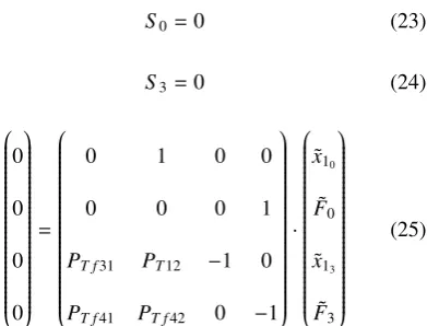
With boundary conditions, Eq.(23), (24) and a few modifications, the final equation Eq.(25) used to obtain material properties of the tube (E1andb1) is:
S0=0 (23)
S3=0 (24)
0 0 0 0 =
0 1 0 0
0 0 0 1
PT f31 PT12 −1 0
PT f41 PT f42 0 −1 · ˜
x10
˜
F0
˜
x13
˜ F3 (25)
And elements of this matrix are written in Eq. 26, 27 and 28.
PT f31=PT11+PT12·M·s2 (26)
PT f41=PT21+M·s2·(PT12·M·s2+2·PT11) (27)
PT f42=PT22+PT12·M·s2 (28) Values of Young modulus (E1) and material damping
(b1) of the pipe can be obtained by making determinant of
transfer matrix equal to zero, withs(eigen number) chosen from measurement data.
2.3 Water-filled pipe experiment
Transfer matrix was formulated in a same way as in previ-ous chapter. The process of formulation exceeds the scope of this contribution and as such is not covered. Navier-Stokes and continuity equations were applied so the fi-nal form allows us to enumerate values of bulk viscosity µB and speed of soundc0for water inside pipe. Material
properties obtained by a manner covered in previous chap-ter were used so the Young modulus and damping of pipe are separate properties of structural part and the evaluated bulk viscosity and speed of sound are properties of fluid for a given simulated instance.
0 0 0 0
=PTwater·
˜ Q0 ˜ p0 ˜ Q3 ˜ p3 (29)
Table 1.Mesh size independence test
No. of elements Frequency [Hz] Damping parameter [Hz]
1274 691,45 -5,2292
200 691,45 -5,2292
80 691,45 -5,2292
30 691,45 -5,2293
12 691,62 -5,2319
6 694,04 -5,2686
3 Simulation
The computed model was only water-filled part of a pipe. Simulation was performed using ANSYS Mechanical pro-gram with Acoustics extension. This extension makes acoustic commands accessible in GUI of ANSYS FEM software. According to [7], there should be at least twelve linear elements of mesh per wavelength or six quadratic ones. Number of elements in a cross section of modelled cylinder is not as important as number of elements along the length of pipe, since the modal solution is longitudinal half wave.
The mesh size dependence analysis shows that few hundred quadratic elements is more than sufficient for ac-curate results. Table 1 contains values of simulation one-meter-long pipe meshed with quadratic elements HEX20.
Boundary conditions on the cylindrical surface as well as on the circular top and bottom is rigid wall. The rigid wall is default boundary condition in ANSYS Acoustics and means that acoustic velocity on a selected geometry is zero. In other words, acoustic velocity does not fluctuate and stays constant. Properties of fluid domain were den-sity and viscoden-sity (shear viscoden-sity or volume viscoden-sity), these parameters were same for all simulations. Speed of sound was regressed from an experimental data. The bulk viscosity varied in a range of measured bulk viscosities to encompass needed amount of values and compare them to the experiment.
4 Custom code
Software based on TMM (transfer matrix method) was used to determine if there is any difference in implemen-tation of the bulk viscosity in ANSYS Acoustics and in custom code named FAchar. In Introduction to Acoustic [7], ANSYS states momentum equation with bulk viscos-ityµBEq. (30).
ρ∂vai
∂t =−∇pa+(
4 3µ+µ
B)· ∇(∇ ·v
ai) (30)
100 101 102 103 104 105 10−6
10−6 10−5 10−4 10−3 10−2 10−1 100
Bulk viscosity [Pa·s]
Log
arithmic
decrement
[dB] ANSYSTMM
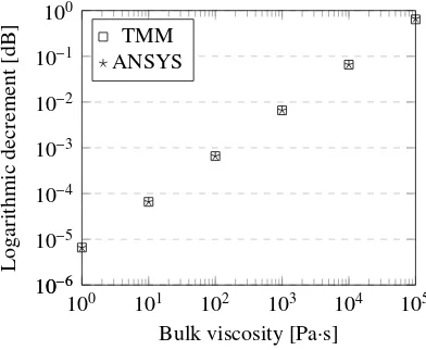
Fig. 2.ANSYS and custom code comparison
Table 2.ANSYS and custom code percental differences (ANSYS minus FAchar and divided by custom code value as a
base)
bulk v. [Pa·s] freq. diff. [%] log. dec. diff. [%]
1 0,00000017 0,138667
10 0,00000017 0,013868
100 0,00000017 0,001387
1000 0,00000017 0,000085
10000 0,00000018 -0,00547
100000 0,006218615 -0,56218
ρ∂vi
∂t =−∇p+∇Πi j (31)
Πi j=µ1
2( ∂vi
∂xj +
∂vj
∂xi)+µ
B∂xi·∂vk
∂xj·∂xk (32)
The computation was performed for both cases on a model of one-meter-long pipe with diameter of 50 mm. Speed of sound was 1500 Pa·s, density 1000 kg·m-3 and bulk viscosities were six values from 1 to 100 000 m2·s-1.
It can be concluded from Figure 2 and Table 2 that with an exception at highest and lowest bulk viscosities the differences in data are very small so author concludes the implementations are sufficiently even and variations come from numeric methods used, discretization and precision.
5 Results
The results compared between the experiment and the sim-ulation are damped frequency and logarithmic decrement of damping. Damped frequency values differ by a few per-cent, frequency obtained from the experiment and
numer-Table 3.Damped frequency comparison; pipe length 1 m, diameter 23 mm
Experiment
Sound speed Frequency Analytic freq.
[m·s-1] [Hz] [Hz]
1381,381578 695,418 690,691
1383,582975 696,510 691,791
1383,567324 696,510 691,784
1383,572992 696,510 691,786
1383,581693 696,510 691,791
1383,58942 696,510 691,795
Acoustic simulation
1387,84 693,905 693,920
1386,085 693,024 693,043
1384,33 692,143 692,165
1382,575 691,261 691,288
1380,82 690,378 690,410
ical model is close to the theoretical frequency value. An-alytical frequency can be calculated for a wave twice as long as a pipe. In Table 3 damped frequencies from ex-periment and simulation are compared to analytical value calculated for given speed of sound. Bigger difference of experimental values is expected result because there are more factors involved and those are omitted in simulation. Logarithmic decrements show very similar trends in relation to bulk viscosity for all pipes but the differences are significantly bigger and up to ten percent. This is doc-umented in Fig. 3, 4 and 5.
6 Discussion
100 101 102 103 104 105 10−6
10−6 10−5 10−4 10−3 10−2 10−1 100
Bulk viscosity [Pa·s]
Log
arithmic
decrement
[dB] ANSYSTMM
Fig. 2.ANSYS and custom code comparison
Table 2.ANSYS and custom code percental differences (ANSYS minus FAchar and divided by custom code value as a
base)
bulk v. [Pa·s] freq. diff. [%] log. dec. diff. [%]
1 0,00000017 0,138667
10 0,00000017 0,013868
100 0,00000017 0,001387
1000 0,00000017 0,000085
10000 0,00000018 -0,00547
100000 0,006218615 -0,56218
ρ∂vi
∂t =−∇p+∇Πi j (31)
Πi j=µ1
2( ∂vi
∂xj +
∂vj
∂xi)+µ
B∂xi·∂vk
∂xj·∂xk (32)
The computation was performed for both cases on a model of one-meter-long pipe with diameter of 50 mm. Speed of sound was 1500 Pa·s, density 1000 kg·m-3 and bulk viscosities were six values from 1 to 100 000 m2·s-1.
It can be concluded from Figure 2 and Table 2 that with an exception at highest and lowest bulk viscosities the differences in data are very small so author concludes the implementations are sufficiently even and variations come from numeric methods used, discretization and precision.
5 Results
The results compared between the experiment and the sim-ulation are damped frequency and logarithmic decrement of damping. Damped frequency values differ by a few per-cent, frequency obtained from the experiment and
numer-Table 3.Damped frequency comparison; pipe length 1 m, diameter 23 mm
Experiment
Sound speed Frequency Analytic freq.
[m·s-1] [Hz] [Hz]
1381,381578 695,418 690,691
1383,582975 696,510 691,791
1383,567324 696,510 691,784
1383,572992 696,510 691,786
1383,581693 696,510 691,791
1383,58942 696,510 691,795
Acoustic simulation
1387,84 693,905 693,920
1386,085 693,024 693,043
1384,33 692,143 692,165
1382,575 691,261 691,288
1380,82 690,378 690,410
ical model is close to the theoretical frequency value. An-alytical frequency can be calculated for a wave twice as long as a pipe. In Table 3 damped frequencies from ex-periment and simulation are compared to analytical value calculated for given speed of sound. Bigger difference of experimental values is expected result because there are more factors involved and those are omitted in simulation. Logarithmic decrements show very similar trends in relation to bulk viscosity for all pipes but the differences are significantly bigger and up to ten percent. This is doc-umented in Fig. 3, 4 and 5.
6 Discussion
Discrepancy in measurement and simulation data could be attributed to various causes. As already stated, in com-putation there is omission of pipe structure, so simulation has no influence of wall thickness, mass of flanges and measuring apparatus or damping in pipe material. In ex-periment a bending of pipe occurs and that is not imple-mented in simulation as well. Also, even small amount of air trapped in pipe can alter measured data [1]. Dissipa-tion of energy caused by vibraDissipa-tions of pipe in air is another neglected effect.
1.5 2 2.5 3 3.5
·104 5·10−2
6·10−2 7·10−2 8·10−2 9·10−2 0.1 0.11 0.12
Bulk viscosity [Pa·s]
Log
arithmic
decrement
[dB] ExperimentANSYS
Fig. 3. ANSYS and experiment; pipe length 2 m; diame-ter 32 mm
43,000 5,000 6,000 7,000 8,000 9,000 4
5 6 7 ·10−2
Bulk viscosity [Pa·s]
Log
arithmic
decrement
[dB] ExperimentANSYS
Fig. 4. ANSYS and experiment; pipe length 1 m; diame-ter 32 mm
1.5 2 2.75 3.5 4
·104 1
2 3 4 5 ·10−2
Bulk viscosity [Pa·s]
Log
arithmic
decrement
[dB] ExperimentANSYS
Fig. 5. ANSYS and experiment; pipe length 6 m; diame-ter 42,5 mm
7 Conclusion
Paper has described measurement of bulk viscosity and part of the mathematical model needed to evaluate data from obtained values of accelerations and pressure pulsa-tions. Acquired bulk viscosities and eigen numbers were used with simulation. Ability to simulate model with bulk viscosity in ANSYS Acoustic and custom code is pre-sented and results show conformity to measured values. Experiment and simulation vary, but given the simplifica-tion of computed model, it can still be considered good fit. Overall conclusion to be made is that acoustic simula-tion with bulk viscosity can yield results with acceptable precision.
Further work could focus on Fluid Structure interac-tion to take structural part into account and improve fi-delity of modeled hydraulic system.
Acknowledgements
This work was supported by NETME Centre, regional R&D cen-tre built with the financial support from the Operational Pro-gramme Research and Development for Innovations within the project NETME Centre (New Technologies for Mechanical En-gineering), Reg.no. CZ.1.05/2.1.00/01.0002 and, in the follow-up sustainability stage, sfollow-upported through NETME CENTRE PLUS (LO1202) by financial means from the Ministry of Edu-cation, Youth and Sports under the “National Sustainability Pro-gramme I” and from the 2017 Science fund of Faculty of Me-chanical engineering, Brno University of Technology project id.: FV 17-25.
Nomenclature
b1 [N s m−1] damping of a pipe
c0 [m s−1] speed of sound
E1 [Pa] stiffness constant of a pipe
F [N] force
M [kg] mass
p [Pa] pressure
pa [Pa] acoustic pressure, amplitude of fluctuation
P transfer matrix
Q [m3s−1] discharge
s [s−1] parameter of Laplace transform
S [m2] area
Sp [m2] area of cross-section
u state vector
v [m s−1] velocity
va [m s−1] acoustic velocity
x [m] dimension coordinate ρ [kg m−3] density
σ [Pa] stress µ [Pa s] viscosity µB [Pa s] bulk viscosity
References
1. HIMR D., HABÁN V.. Simulation of low pres-sure water hammer. IOP Conference Series: Earth and Environmental Science. 2010, 12, 012087-. DOI: 10.1088/1755-1315/12/1/012087. ISSN 1755-1315. 2. GRAVES R. E., ARGROW. B. M.. Bulk Viscosity:
Past to Present. Journal of Thermophysics and Heat Transfer. 1999, 13(3), 337-342. DOI: 10.2514/2.6443. ISSN 0887-8722.
3. POCHYLÝ F., HABÁN V., FIALOVÁ S.. Bulk vis-cosity – constitutive equations.International Review of Mechanical Engineering, September 2011, Vol. 5 n. 6, pp. 1043-1051. ISSN: 1970-8734.
4. KORECK J., MAESS M., GAUL L.. Acoustic-Structure Simulation of Passive Fluid Pulsation Dampers, Fortschritte der Akustik: Plenarvorträge
und Fachbeiträge der 33. Deutschen Jahrestagung für Akustik, DAGA 2007, Stuttgart. Berlin: DEGA, 2007. ISBN: 978-3-9808659-3-7.
5. EISINGER F. L., SULLIVAN R. E.. Vibration Fatigue of Centrifugal Fan Impeller Due to Structural-Acoustic Coupling and Its Prevention: A Case Study.Journal of Pressure Vessel Technology.2007, 129(4), 771-. DOI: 10.1115/1.2767371. ISSN 00949930.
6. JONES P., KESSISSOGLOU N.. (2009). An evalua-tion of current commercial acoustic FEA software for modelling small complex muffler geometries: Predic-tion vs experiment. Annual Conference of the Aus-tralian Acoustical Society 2009 - Acoustics 2009: Re-search to Consulting.