www.ijiset.com
On Suitable Copula Selection with Copula
Garch Method
Ayşe METİN KARAKAŞ
Bitlis Eren University, Department of Statistics, Faculty of Art and Science, 32T[email protected]32T
Abstract
Copula function represents a method which defines the dependence structure of multivariate random variable and it is one of the most important new tools in finance. In this paper, we use combination of copula function and Garch model initially. Afterwards, two-step Copula-GARCH model is used to analyze the dependence structure of data sets. In the first step, we try to obtain standart residuals and construct marginal distributions. In this section, we take into account GARCH (1,1) with standardized Student-t (GARCH). In the second step, for dependence structures of the data sets, we calculate Kendall Tau and Spearman Rho which are nonparametric. With the help of this method, copula parameters are obtained. 0T By means of the 0T
maximum-likelihood estimation method, we get likelihood values for copula families. These values, Akaike information criteria (AIC) and Schwartz information criteria (SIC), are used to determine which copula is suitable for the data set.
Key Words: Akaike information criteria; Copula Function; GARCH method; Kendall Tau; Schwartz information criteria; Spearman Rho.
1. Introduction
Copulas are multivariate uniform distributions. They represent a way of trying to extract the dependence structure from the joint distribution function and to separate dependence and marginal behavior. The main aim of this paper is to it a multivariate distribution to given data. Since a copula function is such a multivariate distribution, it is the perfect tool to do this. A copula can be considered to represent the dependence structure in a distribution, and if fitting, the dependence structure in the data. Copulas represent a useful approach to understanding and modeling dependent random variables. They allow us to focus explicitly on the dependence structure. In recent years, the standard method of estimating dependence has been Pearson’s correlation coefficient, which is based on the multivariate Gaussian distribution. However, as Fama (1963) noted, financial time series do not provide the assumption of normality. That is to say there was a need for the establishment of new
methods to overcome the drawbacks of Person’s correlation coefficient. Multivariate GARCH models formed such a status. The aim of this model is modeling of the conditional covariance and conditional correlation matrix. Sklar (1973) formed structure and properties of a copulas their connection with random variables. Christian Genest and John Mackay (1986) showed how copulas can be used the existence of distribution with singular components and to give a relation with Kendall Tau. Christian Genest and Louis-Paul Rivest (1993) proposed the problem of selecting Archimedean copula providing suitable representation of the dependence structure between two variables. Ana Tustel et.al. (1997) obtained distribution-free multivariate Kolmogorov -Smirnov goodness of fit test. Nelsen (1999) examined copula and properties of copula theory. Eric Bouye et.al. (2000) were used extensively copulas in finance. Rudiger Frey et. al. (2001) modelled credit portfolio loses with copula. Gunky Mervyn J. Silvapulle and Paramsoty (2007) worked ML and IFM methods compared with SP method. Christian Genest and Anne-Catherine Favre (2007) worked to inference for copulas based on rank methods and Salvadori et.al. (2007) used copula to model extremes in nature.
Du, Jiangze, and Kin (2017) search the dependence between electricity spot markets of France, Germany, Austria and Switzerland based on copula models. In this study, the daily exchanges in dependency structure of the dollar, euro and sterling taken from the Central Bank of the Republic of Turkey between 1999 and 2018 years are examined by the Copula GARCH method.
2. Materials and Methods
2.1. GARCH Model. GARCH model was first founded by generalizing ARCH model by Bollerslev and Eagle (1986). The GARCH (p,q) includes p lags of the variances in the linear ARCH (q) conditional variance equation. The variance equation can be generalized as:
2 2 2
1 1
q p
w
t j j t j i i t i
σ = + ∑ α ε + ∑ β σ −
−
= = (1)
www.ijiset.com Another extension is the generalized ARCH or
GARCH model. The GARCH model adds lags of the variance, ht-p, to the standard ARCH. A GARCH (1, 1) method refers to the presence of a first-order autoregressive ARCH statement and a first-order moving average GARCH statement. For GARCH (p,q),
ε
t is the error terms from the meanequation
ε σ
t=
tZ
t, here,Z
t is separatestochastic piece and also
Z
t is residual series,Z
t have zero mean identical and independentdistribution,
σ
t is a time dependent standarddeviation.
β
i ≥0,α
j ≥0 and 11 1
p q
i j
i∑=
β
+ j∑=α
< . 2
1 p
i t i
i∑= β σ − shows GARCH statements,
2 1
q
j t j
j∑=
α σ
− shows ARCH statements. The parameter of ARCH statements and
GARCH statements submit the influence of ARCH effect (past innovation) and GARCH effect on the conditional variance. The rate of this affects the coming periods respectively. In general, GARCH (1,1) is enough to be used for this series [12,13].
2.2. Copula Theory. The copula is defined by a 2
: [0,1] [0,1]
C → which holds the following
conditions
C u
( )
, 0 =C( )
0,u =0 and( )
,1( )
1, , 0,1[ ]
C u =C u = ∀ ∈u u .
(u u1, 2 1 2,v v, )∈[0,1] ,4 such that ,
1 2 1 2
u ≤u v ≤v
(
) (
)
(
) (
)
, ,
2 2 2 1
, , 0.
1 2 1 1
C u v C u v
C u v C u v
−
− + ≥
Ultimately, for twice differentiable and 2-increasing property can be replaced by the condition
2 ( , )
( , ) C u v 0
c u v
u v
∂
= ≥
∂ ∂ (2)
where c u v( , ) is the copula density. For 𝑛-uniform
random U U1, 2, ...,U n variables, the joint
distribution function C is defined by
(
)
(
)
, , , ,
1 2
, , .
1 1 2 2
C u u un
P U u U u Un un
θ …
= ≤ ≤ … ≤
Here θ is dependence parameter
[2,3,4,5,6,7,8,9,10,11,15,16,17,18,19,20,21,22,23,2 4,25,26,27].
2.2.1. Sklar Theorem. Let X and Y be random
variables with continuous distribution functionsFX and FY , which are uniformly distributed on the interval [0,1]
.
Then, there is a copula such that for all ,x y∈R,FXY
( )
X Y, =C F( X( ) ( )
X ,FY Y . (3)The copula C for
(
X Y,)
is the joint distribution function for the pairFX( )
X ,FY( )
Y provided FXandFYcontinuous
[2,3,4,5,6,7,8,9,10,11,15,16,17,18,19,20,21,22,23,2 4,25,26,27].
2.2.2. Plackett Copula. This copula function is defined by
( , )
2
1 ( 1) [1 ( 1)( )] 4 ( 1)
2( 1)
C u v
u v uv
θ θ θ θ
θ
+ − − + − + − −
=
−
(4)
where θ is the copula parameter restricted to
(0, )∞ [25].
2.2.3. Galambos’s Copula. This copula is defined as follows:
{
1/}
( , ) exp (1 ) (1 )
C u v uv u v
θ
θ θ −
− −
=
− + −
(5)for θ ≥0 [25].
2.2.4. Archimedean Copula. Let 𝜑 defines a
functionφ: [0,1]→[0,∞] which is continuous and provides the following conditions;
www.ijiset.com φ(1)=0, (0)φ = ∞.
For all t∈(0,1),
φ
'( )t <0 ,ϕ
is decreasing, for allt∈(0,1)ϕ′′( )
t ≥0 ,ϕ
is convex.ϕ
has an inverseϕ
−1: 0,[ ] [ ]
∞ → 0,1 which hasthe same properties out of
φ
( 1)− (0)=1 and( 1)
( ) 0.
φ
− ∞ = The Archimedean Copula is defined byC u v( , )=φ( 1)− [ ( )φ u +φ( )].v
(6) [25].
2.2.5. Gumbel Copula. This Archimedean copula is definedwith the help of generator function
( ) ( )
t lnt θ
φ = − ,θ≥1;
(
1)
( , ) exp [( ln ) ( ln ) ]
Cθ u v = − − uθ + − vθ θ (7)
whereθ is the copula parameter restricted to
[1, )∞ This copula is asymmetric, with more weight in the right tail. Beside this, it is extreme value copula [25].
2.2.6. Clayton Copula. This Archimedean copula
is defined with the help of generator function 1
( )t t θ φ
θ − −
= ,
Cθ( , )u v =(u−θ +v−θ −1) (8)
where θ is the copula parameter restricted to
(0,∞). This copula is also asymmetric, but with more weight in the left tail [25].
2.2.7. Frank Copula. This Archimedean copula is
defined with the help of generator function;
( )
1ln ;
1
t e t
e
θ
φ
= − − −θ
−− −
( )
1(
(
1)(
)
1)
, ln 1
1
u v
e e
C u v
e
θ θ
θ θ θ
− − − −
= − + −
−
(9)
whereθ is the copula parameter restricted to
( )
0,∞ [25].2.2.8. Joe Copula. This Archimedean copula is
defined with the help of generator function;
( )
t ln 1( )
1 t θ ϕ = −
− −
( )
( ) ( ) ( ) ( )
,1/
1 1 1 ( 1 1
C u v
u v u v
θ
θ
θ θ θ θ
= −
− + − − − −
(10)
where θ is the copula parameter restricted to
[ ]
1,∞ .This copula family is similar to the Gumbel. The right tail positive dependence is stronger than Gumbel [25].2.3. Measuring Dependence
2.3.1. Spearman Rho. Similar to approach of
Pearson correlation coefficient, to compute the correlation between the pairs (R Si, i) of ranks have been used. Thus, Spearman’s Rho
( )( )
1
[ 1,1]
2 2
( ) ( )
1 1
n
Ri R Si S i
n n n
Ri R Si S
i i
ρ
∑ − −
=
= ∈ −
∑ − ∑ −
= =
(11)
where
1 1 1
1 2 1
n n n
R Ri Si
i i
n n
+
∑ ∑
= = =
= = (12)
write. This coefficient that stated expediently in the form
12 3 1
1
( 1)( 1) 1
n n
R S
n i i
i
n n n n
ρ = ∑ − +
=
+ − − (13)
Also,ρn is asymptotically unbiased estimator of
12 ( , ) 3
2 [0,1]
12 ( , ) 3
2 [0,1]
uvdC u v
C u v dudv
ρ = ∫ −
= ∫ − (14)
www.ijiset.com where the second equality is obtained. This
statement can be extended as;
12 ( , ) 3
2 [0,1]
12 1
3
1 1 1 1
uvdCn u v
n Ri Si n n i
n n n n ρ
=
− ∫
− − = ∑
= + + +
(15)
and Cn →C as
n
→ ∞
.Here the null hypothesis0
H =C= Π of independence of XandY , the
distribution of
ρ
n is normal with zero mean andvariance 1 (n−1),thus for H0 approximate
0.05
α = , 1 1, 96
/2
n−
ρ
n >zα
= [4,5,6,7,8].2.3.2. Kendall Tau. Another measure of dependence is Kendall Tau. This measure is based on ranks given by
4 1
( 1) 2
Pn Qn
P
n n
n n n
τ = − = −
−
(16)
where Pn and Qn are number of concordant and discordant pairs respectively. Here,
(X Yi, i), (Xj,Yj) are concordant
(Xi −Xj)(Yi−Yj)>0and these are
disconcordant (Xi−Xj)(Yi −Yj)<0.If
(Xi −Xj)(Yi−Yj)>0; we can say
(Ri −Rj)(Si −Sj)>0.
τ
n is function of copulaCn. As
n
→ ∞
,Cn →C,{
}
1 1
# : ,
1
n
W Iij j Xj X Yi j Yi j
n n
= ∑ = ≤ ≤
= ,
3 4
1 1
4 ( , ) ( , ) 1 2
[0,1]
n n
W n
n n
C u v dC u v
τ = − +
− −
= ∫ −
(17) n
τ
is asymptotically unbiased estimator ofτ
andn
τ
is normal with zero mean and variance2(2n+5) {9 (n n−1)}. Here the null hypothesis 0
H =C= Π of independence of XandY , thus for
0
H approximate
0.05, 9 (n n 1) 2(2n 5) n 1.96
α = − + τ >
[4,5,6,7,8,14].
2.4. Copula estimation
2.4.1. Maximum Likelihood Method (MLE). Maximum likelihood method is commonly used for copula. The aim of this method is basic to find the parameters that make the likelihood functions get its maximum value. It is given
( 1, 2, ..., )
( 1 1( ), 2( 2), ..., ( )) ( ) 1 f x x xn
n c F x F x Fn xn fj xj
j∏ =
=
(18)
Let
{
1 , 2 , ...,}
1T xt x t xnt
t= is the sample data matrix. The likelihood functions can be given
( ) ln( ( 1 1( ), 2( 2 ), ..., ( ))
1
ln ( )
1 1
T
l c F xt F x t Fn xnt t
T n
fj xjt t j
θ = ∑ =
+ ∑ ∑
= =
(19)
Accordingly, the maximum likelihood estimator is ˆ max ( )l
MLE
θ θ
θ
= .
[1,4,5,6,7,8].
2.4.2. Inference for marginal (IFM)
This method is used to overcome the drawbacks of full maximum likelihood function. The aim of copula theory is a separation between the univariate margins and the dependence structure. From equation (19), we write
www.ijiset.com
( )
ln( ( 1 1( , 1), 2( 2 , 2), ..., ( , ), ) 1
ln ( , )
1 1
l
T
c F xt F x t Fn xnt n t
T n
fj xjt j t j
θ
θ θ θ α
θ ∑
= =
∑ ∑ +
= =
(20)
write. In this equation, the vector of the parameters for the univariate marginal is
θ
=(θ θ
1, 2, ...,θ
n) andα
is vector parameters of copula. Accordingly, the fundamental idea of inference for margins is that it forecasts the parameters for marginal distributions and copula separately in two stages. Estimate the parameters
θ
j frommarginal distributions,
ˆ arg max ln ( ; )
1 T
f x
j t j jt j
t
θ θ
θ
= ∑
= (21) Estimation of the vector of the copula
parameters
α
, used the ˆ (ˆ, ˆ , ..., ˆ )1 2 n
θ
=θ θ
θ
;ˆ
ˆ ˆ ˆ
arg max ln( ( 1(1 , 1), 2( 2 , 2), ..., ( , ); )
1
IFM T
c F xt F x t Fn xnt n
t
α
θ θ θ α
α ∑
=
=
(22)
[1,4,5,6,7,8].
2.5. Tail Dependence of Copulas
In order to estimate the copula from bivariate observational data sets, we use the tail dependence concept. It is related to the amount of dependence in the upper-right quadrant tail or in the lower-left-quadrant tail of a bivariate distribution. The upper and lower tail dependence parameter; if a bivariate copula C is such that; it is that upper tail dependence written as;
lim 1 2 ( , )
1 (1 ) v C v v U v
v
λ = − +
→ − (23)
Similarly, lower tail dependence is written as;
lim ( , ) 0
C v v L v
v
λ =
→ (24)
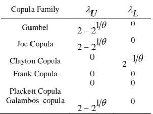
Table 2. For copula families upper and lower tail dependence
Copula Family
U
λ λL
Gumbel 2−21θ 0
Joe Copula 2−21θ 0
Clayton Copula 0 2−1θ
Frank Copula 0 0
Plackett Copula Galambos copula
0
1 2−2 θ
0
0
[1,4,5,6,7,8,25].
2.6. Copula-GARCH Estimation
There are some approaches to model dependence. Many researchers prefer multivariate normal and t distribution to model in applications and GARCH model is widely used in this application. So, we prefer copula instead of multivariate GARCH to model dependence. The most important feature of copula is not requiring any assumptions of the margins normal distribution. Besides, copula permit to separate a high dimensional joint distribution into its marginal distributions and copula function use to link them together. For GARCH model, there are many parameters of which estimation is more difficult. Compare to multivariate GARCH models and other multivariate models, copula is more suitable to model dependence structure. For the series, to model dependence structure, other selection criteria are Akaike’s information criterion (AIC) and Schwarz’s criterion (SIC). These are given as follows;
AIC= −2 logL+2k (25)
SIC = −2 logL+kln( )n (26)
where, k is the number of estimated parameter for each model, n is size of sample [20,21,22].
3. Results and Discussion
3.1. Data Description
In this study, we used data set exchange rate of dollar, euro and sterling get from Central Bank of the Republic of Turkey between 1999 and 2018 years. Wedefine the log-returns of dollar, euro and sterling series. Table 3 and Table 4 contain respectively descriptive statistics of dollar euro and sterling series and dollar, euro and sterling return series. As submitted in these results, the means of
www.ijiset.com dollar, euro, and sterling series are not nearby to
zero and standard deviations are a little bit. The Skewness means that of dollar, euro, and sterling series are positive. The Kurtosis of dollar, euro, and sterling series are positive. The meaning of positive skewness is that of dollar, euro, and sterling series have the longer right tail of density.
Table 3: Descriptive statistics of Euro, Dollar and Sterling series
Dollar Euro Sterling
mean 1,614873 1,967411 2,589657
median 1,490000 1,900000 2,520000
maximum 3,870000 4,140000 4,850000
minimum 0,367383 0,397509 0,590000
Std.dev. 0,643176 0,767270 0,875590
Skewness 0,843414 0,030616 0,027904
Kurtosis 4,224579 2,953051 3,399367
Jarque-Bera 819,0289 1,122239 30,65175
Table 4: Descriptive statistics of Dollar Euro and Sterling return series
Dollar Euro Sterling
mean -0,007332 -0,000379 0,002451
median 0,008150 -0,035048 -0,008549
maximum 5,858241 7,341030 5,238800
minimum -6,040652 -6,934251 -5,860342
Std.dev. 1,765448 1,880493 1,707246
Skewness 0,004231 0,155597 0,139830
Kurtosis 3,739595 3,666246 3,727014
Jarque-Bera 9,095071 8,989556 10,08736
3.2. Modeling the marginal distribution
In table 5, we give marginal modeling for dollar, euro and sterling return series. In these tables, there are coefficients for variance equation. In the
equation (1) αis ARCH (1) and βis GARCH (1).
According to this equation, the sum of the ARCH and GARCH coefficients ( α β+ <1 ) is very close to one, indicating that volatility shocks for these series are quite persistent. This result is often observed in high frequency data.
3.3. With Copula Modeling of the Dependence Structure
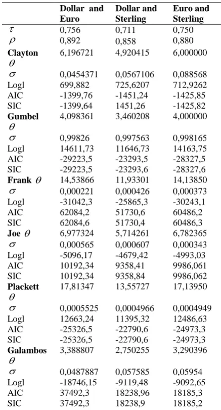
In this study, to model dependence, we present Joe, Gumbel, Clayton, Frank, Plackett and Galambos copula families. We selected Kendall’s Tau and Spearman’s Rho rank correlation statistics in our study, so the correlations parameters corresponding to each copula were obtained based on Kendall’s Tau and Spearman’s Rho. Maximum Likelihood Estimation method is used for application for estimation of copula parameters. Accordingly, in table 6 for copula families, parameter values and
Logl, AIC and SIC values are calculated.
According to these values, with the help of equation (18), (25) and (26), in table 6, relationship of Dollar and Euro series is positive and has a strong relation and based on the AIC and SIC value, we conclude that dependence structure of Dollar and Euro series is modeled by Gumbel copula (θ =4, 098361), in table 6, relationship of Dollar and Sterling series has a positive strong relation and based on the AIC and SIC value, we conclude that dependence structure of Dollar and Sterling series is modeled by Gumbel copula (θ =3, 460208), similarly in table 6, relationship of Euro and Sterling series has a positive strong relation based on the AIC and SIC value, we conclude that dependence structure of Euro and Sterling series is modeled by Gumbel (
4 θ = ).
Table 6: Dollar, Euro and Sterling Series Dependence Structure Modeling
Dollar and Euro
Dollar and Sterling
Euro and Sterling
τ
0,756 0,711 0,750ρ 0,892 0,858 0,880 Clayton
θ 6,196721 4,920415 6,000000 σ 0,0454371 0,0567106 0,088568 Logl 699,882 725,6207 712,9262 AIC -1399,76 -1451,24 -1425,85 SIC -1399,64 1451,26 -1425,82 Gumbel
θ 4,098361 3,460208 4,000000 σ 0,99826 0,997563 0,998165 Logl 14611,73 11646,73 14163,75 AIC -29223,5 -23293,5 -28327,5 SIC -29223,5 -23293,6 -28327,6 Frank θ 14,53866 11,93301 14,13850
σ 0,000221 0,000426 0,000373 Logl -31042,3 -25865,3 -30243,1 AIC 62084,2 51730,6 60486,2 SIC 62084,6 51730,4 60486,3 Joe θ 6,977324 5,714261 6,782365
σ 0,000565 0,000607 0,000343 Logl -5096,17 -4679,42 -4993,03 AIC 10192,34 9358,41 9986,061 SIC 10192,34 9358,84 9986,062 Plackett
θ 17,81347 13,55727 17,13950 σ 0,0005525 0,0004966 0,0004949 Logl 12663,24 11395,32 12486,63 AIC -25326,5 -22790,6 -24973,3 SIC -25326,5 -22790,6 -24973,3 Galambos
θ 3,388807 2,750255 3,290396 σ 0,0487887 0,057585 0,05954 Logl -18746,15 -9119,48 -9092,65 AIC 37492,3 18238,96 18185,3 SIC 37492,3 18238,9 18185,2
www.ijiset.com
Dollar return Series Marginal Modeling Euro return Series Marginal Modeling Sterling return Series Marginal Modeling
Student-t Standard Error Student-t Standard Error Student-t Standard Error ARCH (1) 0,137879 0,012803 0,127816 0,012639 0,172831 0,016884 GARCH(1) 0,851743 0,011022 0,853278 0,012649 0,785212 0,014878
LogL 15674,63 - 15740,60 - 15538,95 -
AIC -6,928868 - -6,958038 - -6,868868 -
SIC -6,921774 - -6,950044 - -6,861778 -
Table 5: Dollar return Series, Euro return Series and Sterling return Series Marginal Modeling.
4. Conclusion
In this paper, we investigated the structure of dependence between Dollar, Euro and Sterling and the data was gotten from Central Bank of the Republic of Turkey. We used Copula- GARCH approach. Primarily, we form the marginal
distribution by using GARCH (1,1) method with
Student-t distribution. From these observed results, Dollar Euro and Sterling series have close and have high frequency data. Also, these series have a strong relationship. For dependency structure between Dollar, Euro and Sterling series, Joe, Gumbel, Clayton, Frank Plackett and Galambos copula functions were used. As can be observed from data sets, series have strong correlation at high values. For this reason, it has been observed that Gumbel copula is suitable to be used for the structure of dependence between Dollar Euro and Sterling. According to this, the dependence of Dollar and Euro is modeled by Gumbel copula, copula with the parameter value of 4,098361, Kendall Tau 0,0756 and Spearman Rho 0,892, for the dependence of Dollar and Sterling suitable copula is Gumbel copula with the parameter value of 3,460208, Kendall Tau 0,711 and Spearman Rho 0,858. Likewise, for the dependence of Euro and Sterling series are the best copula is Gumbel Copula with the parameter value of 4, Kendall Tau 0,750 and Spearman Rho 0,880.
5. Discussion
Investors should take into account the data sets while making financial decisions. According to our study to avoid risk, investors who bought dollar, euro and sterling should also buy other currencies and other investment tools. This is because since the correlations between these currencies are high, investors should notice that the currencies mentioned above have similar tendencies to go up and down. Risk averse investors should take into account this situation and diversify their investment tools.
Also, the currencies have a positive correlation and this situation is good for world economics. Since the buying power of dollar, euro and sterling has
similar tendencies of up and down movements, the import and export of the dollar, euro and sterling using countries will not be negatively affected within each other. This situation is good for world trade and the stability of the economies.
References
[1] Justel, Ana, Daniel Peña, and Rubén Zamar. "A multivariate Kolmogorov-Smirnov test of goodness of fit." Statistics & Probability Letters 35.3 1997: 251-259.
[2] Sklar, Abe. "Random variables, joint
distribution functions, and copulas." Kybernetika 9.6 1973: 449-460.
[3] Caillault, Cyril, and Dominique Guegan.
"Empirical estimation of tail dependence using copulas: application to Asian markets." Quantitative Finance 5.5 2005: 489-501.
[4] Genest, Christian, and Jock MacKay. "The joy of copulas: Bivariate distributions with uniform marginals." The American Statistician 40.4 1986: 280-283.
[5] Genest, Christian, and Louis-Paul Rivest. "Statistical inference procedures for bivariate Archimedean copulas." Journal of the American Statistical Association 88.423 1993: 1034-1043.
[6] Genest, Christian, and Anne-Catherine Favre. "Everything you always wanted to know about copula modeling but were afraid to ask." Journal of hydrologic engineering 12.4 2007: 347-368.
[7
]
Genest, Christian, and Bruno Rémillard. "Validity of the parametric bootstrap for goodness-of-fit testing in semiparametric models." Annales de l'Institut Henri Poincaré, Probabilités et Statistiques. Vol. 44. No. 6. Institut Henri Poincaré, 2008.www.ijiset.com
[8
]
C. Genest, B. Rémillard, & D. Beaudoin,Goodness-of-fit tests for copulas: A review and a power study. Insurance: Mathematics and economics, 44.2 2009: 199-213.
[9] Berg, Daniel. "Copula goodness-of-fit testing: an overview and power comparison." Copulae and Multivariate Probability Distributions in Finance. Routledge, 2013. 79-106.
[10] Huard, David, Guillaume Évin, and
Anne-Catherine Favre. "Bayesian copula selection." Computational Statistics & Data
Analysis 51.2 2006: 809-822.
[11] Bouyé, Eric, et al. "Copulas for finance-a reading guide and some applications." 2000.
[12]
Engle, Robert F., and Tim Bollerslev."Modelling the persistence of conditional variances." Econometric reviews 5.1 1986: 1-50.
[13] Fama, Eugene F. "Mandelbrot and the stable Paretian hypothesis." The journal of business 36.4 1963: 420-429.
[14] Massey Jr, Frank J. "The Kolmogorov-Smirnov test for goodness of fit." Journal of the American Statistical Association 46.253 1951: 68-78.
[15] Kim, Gunky, Mervyn J. Silvapulle, and Paramsothy Silvapulle. "Comparison of semiparametric and parametric methods for estimating copulas." Computational Statistics & Data Analysis51.6 2007: 2836-2850.
[16] Salvadori, Gianfausto, et al. Extremes in nature: an approach using copulas. Vol. 56. Springer Science & Business Media, 2007.
[17
]
Kojadinovic, Ivan, Jun Yan, and MarkHolmes. "Fast large-sample goodness-of-fit tests for copulas." Statistica Sinica 2011: 841-871.
[18] Kojadinovic, Ivan, and Jun Yan. "A goodness-of-fit test for multivariate multiparameter copulas based on multiplier central limit theorems." Statistics and Computing 21.1 2011: 17-30.
[19] Fermanian, Jean-David. "Goodness-of-fit tests for copulas." Journal of multivariate analysis 95.1 2005: 119-152.
[20] Du, Jiangze, and Kin Keung Lai. "Modeling Dependence between European Electricity Markets with Constant and Time-varying Copulas." Procedia computer science 122 2017: 94-101.
[21] Jordanger, Lars Arne, and Dag Tjøstheim. "Model selection of copulas: AIC versus a cross validation copula information criterion." Statistics & Probability Letters 92 2014: 249-255.
[22] Chan, Ngai-Hang, et al. "Statistical inference for multivariate residual copula of GARCH models." Statistica Sinica 2009: 53-70.
[23] Oh, Dong Hwan, and Andrew J. Patton. "High-dimensional copula-based distributions with mixed frequency data." Journal of Econometrics 193.2 2016: 349-366.
[24] Kumar, Pranesh. "Probability distributions and estimation of Ali-Mikhail-Haq copula." Applied Mathematical Sciences 4.14 2010: 657-666.
[25] Nelsen, Roger B. "An introduction to copulas, vol. 139 of Lecture Notes in Statistics." 1999.
[26] Frey, Rüdiger, Alexander J. McNeil, and Mark Nyfeler. "Copulas and credit models." Risk 10.111114.10 2001.
[27] Cherubini, Umberto, and Elisa Luciano.
"Value ‐at‐ risk Trade‐ o
with Copulas." Economic notes 30.2 2001: 235-256.