Financial Intermediation and Credit Policy
in
Business Cycle Analysis
∗
Mark Gertler and Nobuhiro Kiyotaki
N.Y.U. and Princeton
October 2009
This version: March 2010
Abstract
We develop a canonical framework to think about credit market frictions and aggregate economic activity in the context of the current crisis. We use the framework to address two issues in particular:first, how disruptions in financial intermediation can induce a crisis that affects real activity; and second, how various credit market interven-tions by the central bank and the Treasury of the type we have seen recently, might work to mitigate the crisis. We make use of earlier literature to develop our framework and characterize how very recent literature is incorporating insights from the crisis.
∗Prepared for the Handbook of Monetary Economics. Thanks to Michael Woodford, Larry Christiano, Simon Gilchrist, Chris Erceg, and Ian Dew-Becker for helpful comments. Thanks also to Albert Queralto Olive for excellent research assistance.
1
Introduction
To motivate interest in a paper on financial factors in business fluctuations it use to be necessary to appeal either to the Great Depression or to the experiences of many emerging market economies. This is no longer necessary. Over the past few years the United States and much of the industrialized world have experienced the worst financial crisis of the post-war. The global recession that has followed also appears to have been the most severe of this era. At the time of this writing there is evidence that thefinancial sector has stabilized and the real economy has stopped contracting and output growth has resumed. The path to full recovery, however, remains highly uncertain.
The timing of recent events, though, poses a challenge for writing a Hand-book chapter on credit market frictions and aggregate economic activity. It is true that over the last several decades there has been a robust literature in this area. Bernanke, Gertler and Gilchrist (BGG, 1999) surveyed much of the earlier work a decade ago in the Handbook of Macroeconomics. Since the time of that survey, the literature has continued to grow. While much of this work is relevant to the current situation, this literature obviously did not anticipate all the key empirical phenomena that have played out during the current crisis. A new literature that builds on the earlier work is rapidly cropping up to address these issues. Most of these papers, though, are in preliminary working paper form.
Our plan in this chapter is to look both forward and backward. We look forward in the sense that we offer a canonical framework to think about credit market frictions and aggregate economic activity in the context of the current crisis. The framework is not meant as comprehensive description of recent events but rather as afirst pass at characterizing some of the key aspects and at laying out issues for future research. We look backward by making use of earlier literature to develop the particular framework we offer. In doing so, we address how this literature may be relevant to the new issues that have arisen. We also, as best we can, characterize how very recent literature is incorporating insights from the crisis.
From our vantage, there are two broad aspects of the crisis that have not been fully captured in work on financial factors in business cycles. First, by all accounts, the current crisis has featured a significant disruption offinancial
intermediation.1 Much of the earlier macroeconomics literature withfinancial
frictions emphasized credit market constraints on non-financial borrowers and treated intermediaries largely as a veil (see, e.g. BGG). Second, to combat the crisis, both the monetary and fiscal authorities in many countries including the US. have employed various unconventional policy measures that involve some form of direct lending in credit markets.
From the standpoint of the Federal Reserve, these "credit" policies repre-sent a significant break from tradition. In the post war era, the Fed scrupu-lously avoided any exposure to private sector credit risk. However, in the current crisis the central bank has acted to offset the disruption of inter-mediation by making imperfectly secured loans to financial institutions and by lending directly to high grade non-financial borrowers. In addition, the
fiscal authority acting in conjunction with the central bank injected equity into the major banks with the objective of improving credit flows. Though the issue is not without considerable controversy, many observers argue that these interventions helped stabilized financial markets and, as consequence, helped limit the decline of real activity. Since these policies are relatively new, much of the existing literature is silent about them.
With this background in mind, we begin in the next section by developing a baseline model that incorporatesfinancial intermediation into an otherwise frictionless business cycle framework. Our goal is twofold: first to illustrate how disruptions in financial intermediation can induce a crisis that affects real activity; and second, to illustrate how various credit market interventions by the central bank and the Treasury of the type we have seen recently, might work to mitigate the crisis.
As in Bernanke and Gertler (1989), Kiyotaki and Moore (1997) and oth-ers, we endogenizefinancial market frictions by introducing an agency prob-lem between borrowers and lenders.2 The agency problem works to introduce
a wedge between the cost of external finance and the opportunity cost of
in-1For a description of the disruption of financial intermediation during the current re-cession, see Brunnermeier (2008), Gorton (2008) and Bernanke (2009). For a more general description offinancial crisis over the last several hundred years, see Reinhart and Rogoff (2009).
2A partial of other macro models with financial frictions in this vein includes, Williamson (1987), Kehoe and Livene (1994), Holmstrom and Tirole (1997), Carlstrom and Fuerst (1997), Caballero and Kristhnamurthy (2001), Kristhnamurthy (2003), Chris-tiano, Motto and Rostagno (2005), Lorenzoni (2008), Fostel and Geanakoplos (2009), and Brunnermeir and Sannikov (2009).
ternal finance, which adds to the overall cost of credit that a borrower faces. The size of the external finance premium, further, depends on the condition of borrower balance sheets. Roughly speaking, as a borrower’s percentage stake in the outcome of an investment project increases, his or her incen-tive to deviate from the interests of lenders’ declines. The external finance premium then declines as a result.
In general equilibrium, a "financial accelerator" emerges. As balance sheets strengthen with improved economics conditions, the external finance problem declines, which works to enhance borrower spending, thus enhancing the boom. Along the way, there is mutual feedback between thefinancial and real sectors. In this framework, a crisis is a situation where balance sheets of borrowers deteriorate sharply, possibly associated with a sharp deterioration in asset prices, causing the external finance premium to jump. The impact of the financial distress on the cost of credit then depresses real activity.3
Bernanke and Gertler (1989), Kiyotaki and Moore (1997) and others focus on credit constraints faced by non-financial borrowers.4 As we noted earlier,
however, the evidence suggests that disruption of financial intermediation is a key feature of both recent and historical crises. Thus we focus our attention here on financial intermediation.
We begin by supposing thatfinancial intermediaries have skills in evaluat-ing and monitorevaluat-ing borrowers, which makes it efficient for credit toflow from lenders to non-financial borrowers through the intermediaries. In particular, we assume that households deposit funds in financial intermediaries that in turn lend funds to non-financialfirms. We then introduce an agency problem that potentially constrains the ability of intermediaries to obtain funds from depositors. When the constraint is binding (or there is some chance it may bind), the intermediary’s balance sheet limits its ability to obtain deposits. In this instance, the constraint effectively introduces a wedge between the loan and deposit rates. During a crisis, this spread widens substantially, which in turn sharply raises the cost of credit that non-financial borrowers face.
As recent events suggest, however, in a crisis, financial institutions face
3Most of the models focus on the impact of borrower constraints on producer durable spending. See Monacelli (2009) and Iacoviello (2005) for extensions to consumer durables and housing. Jermann and Quadrini (2009), amongst others, focus on borrowing con-straints on employment.
4An exception is Holmstrom and Tirole (1997). More recent work includes see He and Kristhnamurthy (2009), and Angeloni and Faia (2009).
difficulty not only in obtaining depositor funds in retail financial markets but also in obtaining funds from one another in wholesale ("inter-bank") markets. Indeed, thefirst signals of a crisis are often strains in the interbank market. We capture this phenomenon by subjecting financial institutions to idiosyncratic "liquidity" shocks, which have the effect of creating surplus and deficits of funds acrossfinancial institutions. If the interbank market works perfectly, then funds flow smoothly from institutions with surplus funds to those in need. In this case, loan rates are thus equalized across different
financial institutions. Aggregate behavior in this instance resembles the case of homogeneous intermediaries.
However, to the extent that the agency problem that limits an intermedi-ary’s ability to obtain funds from depositors also limits its ability to obtain funds from other financial institutions and to the extent that nonfinancial
firms can obtain funds only from a limited set of financial intermediaries, disruptions of inter-bank markets are possible that can affect real activity. In this instance, intermediaries with deficit funds offer higher loan rates to nonfinancialfirms than intermediaries with surplus funds. In a crisis this gap widens. Financial markets effectively become segmented and sclerotic. As we show, the inefficient allocation of funds across intermediaries can further depress aggregate activity.
In section 3 we incorporate credit policies within the formal framework. In practice the central bank employed three broad types of policies. Thefirst, which was introduced early in the crisis, was to permit discount window lend-ing to banks secured by private credit. The second, introduced in the wake of the Lehmann default was to lend directly in relatively high grade credit markets, including markets in commercial paper, agency debt and mortgage-backed securities. The third (and most controversial) involved direct assis-tance to large financial institutions, including the equity injections and debt guarantees under the Troubled Assets Relief Program (TARP) as well as the emergency loans to JP Morgan Chase (who took over Bear Stearns) and AIG. We stress that within our framework, the net benefits from these various credit market interventions are increasing in the severity of the crisis. This helps account for why it makes sense to employ them only in crisis situations. In section 4, we use the model to simulate numerically a crisis that has some key features of the current crisis. Absent credit market frictions, the disturbance initiating the crisis induces only a mild recession. With credit frictions (especially those in interbank market), however, an endogenous dis-ruption offinancial intermediation works to magnify the downturn. We then
explore how various credit policies can help mitigate the situation.
Our baseline model is quite parsimonious and meant mainly to exposit the key issues. In section 5, we discuss a number of questions and possible extensions. In some cases, we discuss a relevant literature, stressing the implications of this literature for going forward.
2
A Canonical Model of Financial
Intermedi-ation and Business FluctuIntermedi-ations
Overall, the specific business cycle model is a hybrid of Gertler and Karadi’s (2009) framework that allows for financial intermediation and Kiyotaki and Moore’s (2008) framework that allows for liquidity risk. We keep the core macro model simple in order to see clearly the role of intermediation and liquidity. On the other hand, we also allow for some features prevalent in conventional quantitative macro models (such as Christiano, Eichenbaum and Evans (2005), Smets and Wouters (2007)) in order to get rough sense of the importance of the factors we introduce.5
For simplicity we restrict attention to a purely real model and only credit policies, as opposed to conventional monetary models. Extending the model to allow for nominal rigidities is straightforward (see., e.g., Gertler and Karadi, 2009), and permits studying conventional monetary policy along with unconventional policies. However, because much of the insight into how credit market frictions may affect real activity and how various credit policies may work can be obtained from studying a purely real model, we abstract from nominal frictions.6
5Some recent monetary DSGE models that incorporatefinancial factors include Chris-tiano, Motto, and Rostagno (2009) and Gilchrist, Ortiz and Zakresjek (2009).
6There, however, several insights that monetary models add, however. First, if the zero lower bound on the nominal interest is binding, thefinancial market disruptions will have a larger effect than otherwise. This is because the central bank is not free to further reduce the nominal rate to offset the crisis. Second, to the extent there are nominal price and/or wage rigidities that induce countercyclical markups, the effect of the credit market disruption and aggregate activity is amplified. See, e.g., Gertler and Karadi (2009) and Del Negro, Ferrero, Eggertsson and Kiyotaki (2010) for an illustration of both of these points.
2.1
Physical Setup
Before describing our economy with financial frictions, we present the phys-ical environment.
There are a continuum of firms of mass unity located on a continuum of islands. Each firm produces output using an identical constant returns to scale Cobb-Douglas production function with capital and labor as inputs. Capital is not mobile, but labor is perfectly mobile acrossfirms and islands. Because labor is perfectly mobile, we can express aggregate output Yt as a
function of aggregate capital Kt and aggregate labor hoursLt as:
Yt=AtKtαLt1−α, 0< α <1, (1)
where At is aggregate productivity which follows a Markov process.
Each period investment opportunities arrive randomly to a fractionπi of islands. On a fraction πn = 1
−πi of islands, there are no investment
op-portunities. Onlyfirms on islands with investment opportunities can acquire new capital. The arrival of investment opportunities is i.i.d. across time and across islands. The structure of this idiosyncratic risk provides a simple way to introduce liquidity needs by firms, following Kiyotaki and Moore (2008). Let It denote aggregate investment, δ the rate of physical deprecation and
ψt+1 a shock to the quality of capital. Then the law of motion for capital is given by :
Kt+1 = ψt+1[It+πi(1−δ)Kt] +ψt+1π
n
(1−δ)Kt
= ψt+1[It+ (1−δ)Kt]. (2)
The first term of the right reflects capital accumulated byfirms on investing islands and the second is capital that remains on non-investing islands, after depreciation. Summing across islands yields a conventional aggregate relation for the evolution of capital, except for the presence of the disturbance ψt+1, which we refer to as a capital quality shock. Following the finance literature (e.g., Merton (1973)), we introduce the capital quality shock as a simple way to introduce an exogenous source of variation in the value of capital. As will become clear later, the market price of capital will be endogenous within our framework. In this regard, the capital quality shock will serve as an exogenous trigger of asset price dynamics. The random variable ψt+1 is best thought of as capturing some form of economic obsolescence, as opposed to
physical depreciation.7 We assume the capital quality shockψ
t+1also follows
a Markov process.8
Firms on investing islands acquire capital from capital goods producers who operate in a national market. There are convex adjustment costs in the gross rate of change in investment for capital goods producers. Aggregate output is divided between household consumption Ct, investment
expendi-tures, and government consumption Gt,
Yt=Ct+ [1 +f(
It
It−1
)]It+Gt (3)
wheref( It
It−1)It reflects physical adjustment costs, withf(1) =f
0(1) = 0and
f00(I
t/It−1) > 0. Thus the aggregate production function of capital goods
producers is decreasing returns to scale in the short-run and is constant returns to scale in the long-run.
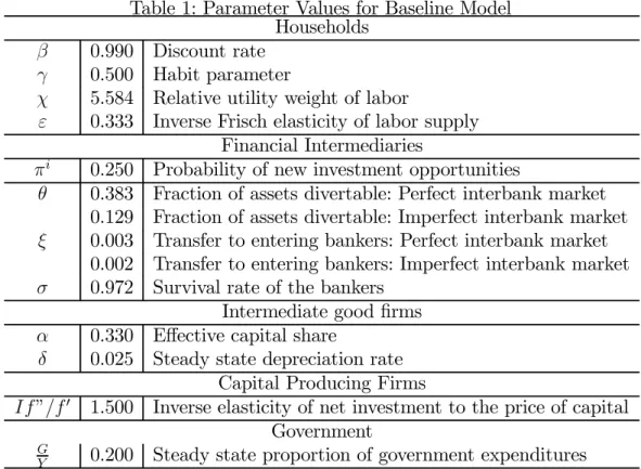
Next we turn to preferences: Et ∞ X i=0 βi ∙ ln(Ct+i−γCt+i−1)− χ 1 +εL 1+ε t+i ¸ (4) where Et is the expectation operator conditional on date t information and
γ ∈(0,1). We abstract from many frictions in the conventional DSGE frame-work (e.g. nominal price and wage rigidities, variable capital utilization, etc.). However, we allow both habit formation of consumption and adjust-ment costs of investadjust-ment because, as the DSGE literature has found, these features are helpful for reasonable quantitative performance and because they can be kept in the model at minimal cost of additional complexity.
If there were no financial frictions, the competitive equilibrium would correspond to a solution of the planner’s problem that involves choosing ag-gregate quantities (Yt, Lt, Ct, It, Kt+1) as a function of the aggregate state
7One way to motivate this disturbance is to assume that final output is a C.E.S. com-posite of a continuum of intermediate goods that are in turn produced by employing capital and labor in a Cobb-Douglas production technology. Suppose that, once capital is installed, capital is good-specific and that each period a random fraction of goods become obsolete and are replaced by new goods. The capital used to produced the obsolete goods is now worthless and the capital for the new goods is not fully on line. The aggregate capital stock will then evolve according to equation. (2).
8Other recent papers that make use of this kind of disturbance include, Gertler and Karadi (2009), Brunnermeier and Sannikov (2009) and Gourio (2009).
(Ct−1, It−1, Kt, At, ψt) in order to maximize the expected discounted utility
of the representative household subject to the resource constraints. This frictionless economy (a standard real business cycle model) will serve as a benchmark to which we may compare the implications of the financial fric-tions.
In what follows we will introduce banks that intermediate funds between households and non-financial firms in a retail financial market. In addition, we will allow for a wholesale inter-bank market, where banks with surplus funds on non-investment islands lend to banks in need of funds on investing islands. We will also introduce financial frictions that may impede credit
flows in both the retail and wholesale financial markets and then study the consequences for real activity.
2.2
Households
In our economy with credit frictions, households lend to non-financial firms viafinancial intermediaries. Following Gertler and Karadi (2009), we formu-late the household sector in way that permits maintaining the tractability of the representative agent approach.
In particular, there is a representative household with a continuum of members of measure unity. Within the household there are 1−f "work-ers" and f "bankers". Workers supply labor and return their wages to the household. Each banker manages afinancial intermediary (which we will call a "bank") and transfers nonnegative dividends back to household subject to its flow of fund constraint. Within the family there is perfect consumption insurance.
Households do not hold capital directly. Rather, they deposit funds in banks. (It may be best to think of them as depositing funds in banks other than the ones they own). In our model, bank deposits are riskless one period securities. Households may also hold riskless one period government debt which is a perfect substitute for bank deposits.
Let Wt denote the wage rate, Tt lump sum taxes, Rt the gross return
on riskless debt from t−1 to t, Dht the quantity of riskless debt held, and Πt net distributions from ownership of both banks and non-financial firms.
Then the household chooses consumption, labor supply and riskless debt
(Ct, Lt, Dht+1) to maximize expected discounted utility (4) subject to the
Ct=WtLt+Πt−Tt+RtDht−Dht+1. (5)
LetuCt denote the marginal utility of consumption andΛt,t+1 the
house-hold’s stochastic discount factor. Then the househouse-hold’sfirst order conditions for labor supply and consumption/saving are given by
EtuCtWt=χLϕt, (6) EtΛt,t+1Rt+1 = 1, (7) with uCt≡(Ct−γCt−1)−1−βγ(Ct+1−γCt)−1 and Λt,t+1 ≡β uCt+1 uCt .
Because banks may be financially constrained, bankers will retain earn-ings to accumulate assets. Absent some motive for paying dividends, they mayfind it optimal to accumulate to the point where thefinancial constraint they face is no longer binding. In order to limit bankers’ ability to save to overcome financial constraints, we allow for turnover between bankers and workers. In particular, we assume that with i.i.d. probability1−σ, a banker exits next period, (which gives an average survival time = 1−1σ). Upon ex-iting, a banker transfers retained earnings to the household and becomes a worker. Note that the expected survival time may be quite long (in our baseline calibration it is ten years.) It is critical, however, that the expected horizon is finite, in order to motivate payouts while the financial constraints are still binding.
Each period, (1−σ)f workers randomly become bankers, keeping the number in each occupation constant. Finally, because in equilibrium bankers will not be able to operate without anyfinancial resources, each new banker receives a "start up" transfer from the family as a small constant fraction of the total assets of entrepreneurs. Accordingly, Πt is net funds transferred
to the household:i.e., funds transferred from exiting bankers minus the funds transferred to new bankers (aside from small profits of capital producers).
An alternative to our approach of having a consolidated family of work-ers and bankwork-ers would be to have the two groups as distinct sets of agents, without any consumption insurance between the two groups. It is unlikely, however, that the key results of our paper would change qualitatively. By
sticking with complete consumption insurance, we are able to have lending and borrowing in equilibrium and still maintain tractability of the represen-tative household approach.
2.3
Banks
To finance lending in each period, banks raise funds in a national financial market. Within the nationalfinancial market, there is a retail market, where banks obtain deposits from households; and a wholesale market, where banks borrows and lend amongst one and another.
At the beginning of the period each bank raises depositsdt from
house-holds in the retail financial market at the deposit rateRt+1. After the retail
financial market closes, investment opportunities for nonfinancial firms ar-rive randomly to different islands. Banks can only make loans to nonfinancial
firms located on the same island. As we stated earlier, for a fraction πi of
locations, new investment opportunities are available to finance as well as existing projects. Conversely, for a fraction πn = 1
−πi, no new investments
are available to finance, only existing ones. On the interbank market, banks on islands with new lending opportunities will borrow funds from those on islands with no new project arrivals.9
Financial frictions affect real activity in our framework via the impact on funds available to banks. For simplicity, however, there is no friction in transferring funds between a bank and non-financial firms in the same island. In particular, we suppose that the bank is efficient at evaluating and monitoring non-financial firms of the same island, and also at enforcing contractual obligations with these borrowers. We assume the costs to a bank of performing these activities are negligible. Accordingly, given its supply of available funds, a bank can lend frictionlessly to non-financial firms of the same island against their future profits. In this regard,firms are able to offer banks perfectly state-contingent debt. It is simplest to think of the bank’s claim on nonfinancial firms as equity.
9Our model is thus one where liquidity problems emerge in part due to limited market participation, in the spirit of Allen and Gale (1995, 2007) and others. This is because within our framework (i) only banks of the same island can make loans to nonfinancial firms and (ii) banks on investing islands cannot raise additional funds in the retailfinancial market after they learn their customers have investment opportunities.
After learning about its lending opportunities, a bank decides the vol-ume of loans sht to make to non-financialfirms and the volume of interbank
borrowing bh
t where the superscript h = i, n denotes the island type (i for
investing and n for non-investing) on which the bank is located during the period. Let Qht be price of a loan (or "asset") - i.e. the market price of the
bank’s claim on the future returns from one unit of present capital of
non-financial firm at the end of period. We index the asset price by h because, owing to temporal market segmentation, Qht may depend on the volume of
opportunities that the bank faces.
For an individual bank, theflow-of-funds constraint implies the value of loans funded within a given period, Qhtsht, must equal the sum of the bank
net worth nh
t, its borrowings on the interbank marketbht and deposits dt:
Qhtsht =nth+bht +dt. (8)
Note thatdt does not depend upon the volume of the lending opportunities,
which is not realized at the time of obtaining deposits.
LetRbt be the interbank interest rate from periodst−1to periodt. Then
net worth at t is the gross payofffrom assets funded att−1, net borrowing costs, as follows:
nht = [Zt+ (1−δ)Qht]ψtst−1−Rbtbt−1 −Rtdt−1, (9)
where Zt is the dividend payment at t on the loans the bank funds at t−1.
(Recall that ψt is an exogenous aggregate shock to the quality of capital). Observe that the gross payoff from assets depends on the location specific asset price Qht, which is the reason nht depends on the realization of the
location specific shock att.
Given that the bank pays dividends only when it exits (which occurs with a constant probability), the objective of the bank at the end of period t is the expected present value of future dividends, as follows
Vt=Et
∞
X
i=1
(1−σ)σi−1Λt,t+inht+i, (10)
where Λt,t+i is the stochastic discount factor, which is equal to the marginal
rate of substitution between consumption of date t+ i and date t of the representative household.
In order to maintain tractability, we make assumptions to ensure that we do not have to keep track of the distribution of net worth across islands.
In particular, we allow for arbitrage at the beginning of each period (before investment opportunities arrive) to ensure that ex ante expected rates of return to intermediation are equal across islands. In particular, we suppose that a fraction of banks on islands where expected returns are low can move to islands where they are high. Before they move, they sell their existing loans to nonfinancial firms to the other banks that remain on the island in exchange for inter-bank loans that the remaining banks have been holding in their portfolios. These transactions keep each existing loan to nonfinancial
firms on the island it was initiated. At the same time, they permit arbitrage to equalize returns across markets ex ante.
As will become clear later, ex ante expected returns being equalized across islands requires that the ratio of total intermediary net worth to total capital on each island be the same at the beginning of each period10. Thus, given
this arbitrage activity and given that the liquidity shock is i.i.d., we do not have to keep track of the beginning of period distribution of net worth across islands.
To motivate an endogenous constraint on the bank’s ability to obtain funds in either the retail or wholesale financial markets, we introduce the following simple agency problem: We assume that after an bank obtains funds, the banker managing the bank may transfer a fractionθof "divertable" assets to his or her family. Divertable assets consists of total gross assetsQh
tsht
net a fraction ω of interbank borrowing bh
t. If a bank diverts assets for its
personal gain, it defaults on its debt and is shut down. The creditors may re-claim the remaining fraction1−θ of funds. Because its creditors recognize the bank’s incentive to divert funds, they will restrict the amount they lend. In this way a borrowing constraint may arise.
We allow for the possibility that bank may be constrained not only in obtaining funds from depositors but also in obtaining funds from other banks. Though we permit the tightness of the constraint faced in each market to differ. In particular, the parameter ω indexes (inversely) the relative degree of friction in the interbank market:
Withω = 1, banks cannot divert assetsfinanced by borrowing from other banks: Lending banks are able to perfectly recover the assets that underlie the loans they make. In this case, the interbank market operates frictionlessly,
10In turn, this requires a movement of net worth from low return to high return islands that is equal in total to the quantity of interbank loans issued in the previous period. The asset exchange between moving and staying banks described in the text accomplishes this arbitrage.
and banks are not constrained in borrowing from one another. They may only be constrained in obtaining funds from depositors.
In contrast, withω = 0,lending banks are no more efficient than depos-itors in recovering assets from borrowing banks. In this case, the friction that constrains a banks ability to obtaining funds on the interbank market is the same as for the retail financial market. In general, we can allow para-meter ω to differ for borrowing versus lending banks. However, maintaining symmetry simplifies the analysis without affecting the main results.
We assume that the banker’s decision over whether to divert funds must be made at the end of the period after the realization of the idiosyncratic uncertainty that determines its type, but before the realization of aggregate uncertainty in the following period. Here the idea is that if the banker is going to divert funds, it takes time to position assets and this must be done between the periods (e.g., during the night). Let Vt(sht, bht, dt) be the
maximized value of Vt, given an asset and liability configuration
¡
sh t, bht, dt
¢
at the end of period t. Then in order to ensure the bank does not divert funds, the following incentive constraint must hold for each bank type:
Vt(sht, b h t, dt)≥θ(Qhts h t −ωb h t). (11)
In general the value of the bank at the end of period t−1 satisfies the Bellman equation Vt−1(st−1, bt−1, dt−1) = Et−1Λt−1,t X h=i,n πh{(1−σ)nht +σM ax dt [M ax sh t,bht Vt(sht, b h t, dt)]}. (12)
Note that the loans and interbank borrowing are chosen after a shock to the loan opportunity is realized while deposits are chosen before.
To solve the decision problem, we first guess that the value function is linear:
Vt(sht, bht, dt) =νstsht −νbtbht −νtdt (13)
whereνst, νbt andνtare time varying parameters, and verify this guess later.
Note that νst is the marginal value of assets at the end of periodt;νbt is the
marginal cost of interbank debt; and νt is the marginal cost of deposits.11 11The parameters in the conjectured value function are independent of the individual bank’s type because the value function is measured after the bankfinishes its transaction for the current this period and because the shock to the loan opportunity is i.i.d. across periods.
Letλht be the Lagrangian multiplier for the incentive constraint (11) faced by bank of typeh andλt≡
P
h=i,n
πhλht be the average of this multiplier across
states. Then given the conjectured form of the value function, we may express thefirst order conditions for dt, sht, and λ
h t, as: (νbt−νt) (1 +λt) =θωλt, (14) µ νst Qh t −νbt ¶ (1 +λht) =λhtθ(1−ω), (15) [θ−(νst Qh t −νt)]Qhts h t −[θω−(νbt−νt)]bht ≤νtnht. (16)
According to equation (14), the marginal cost of interbank borrowing ex-ceeds the marginal cost of deposit if and only if the incentive constraint is expected to bind for some state (λt>0) and the inter-bank market operates
more efficiently than the retail deposit market (i.e., ω >0, meaning that as-setsfinanced by interbank borrowing are harder to divert than thosefinanced by deposits). Equation (15) states that the marginal value of assets in terms of goods νst
Qh
t exceeds the marginal cost of interbank borrowing by banks on type h island to the extent that the incentive constraint is binding (λht >0)
and there is a friction in interbank market (ω <1). Finally, equation (16) is the incentive constraint. It requires that the values of the bank’s net worth (or equity capital), νtnht, must be at least as large as weighted measure of
assets Qh
tsht net of interbank borrowing bht that a bank holds. In this way,
the agency problem introduces an endogenous balance sheet constraint on banks.
The model for the general case with0≤ω≤1is somewhat cumbersome to solve. There are, however, two interesting special cases that provide insight into the models workings. In case 1, there is a perfect interbank market, which arises whenω = 1.In case 2, the frictions in the interbank market are of the same magnitude as in the retail financial market, which arises when ω = 0. We next proceed to characterize each of the cases. The Appendix then provides a solution for the general case of an interbank friction with ω < 1.
2.3.1 Case 1: Frictionless wholesale financial market (ω = 1)
If banks cannot divert assets financed by inter-bank borrowing (ω = 1), in-terbank lending is frictionless. As equation (15) suggests, perfect arbitrage in the interbank market equalizes the shadow values of assets in each market, implying νst
Qb
t =
νst
Ql
t, which in turn implies Q
b
t =Qlt =Qt. The perfect
inter-bank market, further, implies that the marginal value of assets in terms of goods νst
Qt must equal the marginal cost of borrowing on the interbank market νbt,
νst
Qt
=νbt. (17)
Because asset prices are equal across island types, we can drop the h superscript in this case. Accordingly, let μt denote the excess value of a unit
of assets relative to deposits, i.e., the marginal value of holding assets νst
Qt net the marginal cost of deposits νt. Then, given that banks are constrained in
the retail deposit market, equations (14) and (15) imply that the μt≡ νst
Qt −
νt >0. (18)
It follows that the incentive constraint (16) in this case may expressed as Qtst−bt=φtnt (19)
with
φt= νt
θ−μt. (20)
Note that since interbank borrowing is frictionless, the constraint applies to assets intermediated minus interbank borrowing. How tightly the constraint binds depends positively on the fraction of net assets the bank can divert and negatively on the excess value of bank assets, given by μt. The higher the excess value is, the greater is the franchise value of the bank and the less likely it is to divert funds.
LetΩt+1be the marginal value of net worth at date t+1 and letRkt+1 is
the gross rate of return on bank assets. Then after combining the conjectured value function with the Bellman equation, we can verify the value function is linear in ¡sh
t, bht, dt
¢
if μt and νt satisfy:
μt=EtΛt,t+1Ωt+1(Rkt+1−Rt+1) (22) with Ωt+1 = 1−σ+σ(νt+1+φt+1μt+1), and Rkt+1 =ψt+1 Zt+1+ (1−δ)Qt+1 Qt .
Let us define the "augmented stochastic discount factor" as the stochastic discount factorΛt,t+1weighted by the (stochastic) marginal value of net worth
Ωt+1. (The marginal value of net worth is a weighted average of marginal
values for exiting and for continuing banks. If a continuing bank has an additional net worth, it can save the cost of deposits and can increase assets by the leverage ratio φt+1, where assets have an excess value equal to μt+1
per unit). According to (21), the cost of deposits per unit to the bank νt
is the expected product of the augmented stochastic discount factor and the deposit rateRt+1.Similarly from(22), the excess value of assets per unit,μt,
is the expected product of the augmented stochastic discount factor and the excess return Rkt+1−Rt+1.
Since the leverage ratio net of interbank borrowing, φt, is independent
of both bank-specific factors and island-specific factors, we can sum across individual banks to obtain the relation for the demand for total bank assets QtSt as a function of total net worthNt as:
QtSt=φtNt (23)
whereφtis given by equation (20). Overall, a setting with a perfect interbank is isomorphic to one where banks do not face idiosyncratic liquidity risks. Aggregate bank lending is simply constrained by aggregate bank capital.
If the banks’ balance sheet constraints are binding in the retail financial market, there will be excess returns on assets over deposits. However, a perfect interbank market leads to arbitrage in returns to assets across market as follows:
EtΛt,t+1Ωt+1Rkt+1 =EtΛt,t+1Ωt+1Rbt+1 > EtΛt,t+1Ωt+1Rt+1. (24)
As will become clear, a crisis in such economy is associated with an increase in the excess return on assets for banks of all types.
2.3.2 Case 2: Symmetric frictions in wholesale and retailfinancial markets (ω = 0)
In this instance the bank’s ability to divert funds is independent of whether the funds are obtained in either the retail or wholesalefinancial markets. This effectively makes the borrowing constraint the bank faces symmetric in the two credit markets. As a consequence, interbank loans and deposits become perfect substitutes as sources of finance. Accordingly, equation (14) implies that the marginal cost of interbank borrowing is equal to the marginal cost of deposits
νbt =νt. (25)
Here, even if banks on investing islands arefinancially constrained, banks on non-investing islands may or may not be. Roughly speaking, if the constraint on inter-bank borrowing binds tightly, banks in non-investing islands will be more inclined to use their funds to re-finance existing investments rather than lend them to banks on investing islands. This raises the likelihood that banks on non-investing islands will earn zero excess returns on their assets.
Because asset supply per unit of bank net worth is larger on investing islands than on non-investing islands, the asset price is lower, i.e., Qi
t< Qnt.
Intuitively, given that the leverage ratio constraint limits banks’ ability to acquire assets, prices will clear at lower values on investing islands where supplies per unit of bank net worth are greater. In the previous case of a perfect interbank market, funds flow from non-investing to investing islands to equalize asset prices. Here, frictions in the inter-bank market limit the degree of arbitrage, keeping Qit below Qnt.
A lower asset price on the investing island, of course, means a higher expected return. Let μh
t ≡ νst
Qh
t −νt be the excess value of assets on a type h island. Then we have:
μit > μ n
t ≥0. (26)
The positive excess return implies that banks in the investing islands are
finance constrained. Thus the leverage ratios for banks on each island type are given by:
Qitsit ni t =φit = νt θ−μi t (27) Qn tsnt nn t ≤φnt = νt θ−μn t , and µ Qn tsnt nn t −φnt ¶ μnt = 0. (28)
In this case the method of undetermined coefficients yields νt =EtΛt,t+1 X h0=i,n πh0Ωht+10 Rt+1 = Et h0Λt,t+1Ω h0 t+1Rt+1 (29) μht = Et h0Λt,t+1Ω h0 t+1(R hh0 kt+1−Rt+1) (30) with Ωht+10 = 1−σ+σ(νt+1+φh 0 t+1μ h0 t+1), and Rhhkt+10 =ψt+1 Zt+1+ (1−δ)Qh 0 t+1 Qh t .
With an imperfect interbank market, both the marginal value of net worth
Ωh0
t+1 and the return on assets Rhh 0
kt+1 depend on which island type a bank
enters in the subsequent period. Accordingly, we index each by h0 and take expectations over h0 conditional on date t information denoted asE
t h0.
Because leverage ratios differ across islands, we aggregate separately across bank-types to obtain the aggregate relations:
QitSti =φitNti (31) QntStn ≤φntNtn, and (QtnStn−φntNtn)μnt = 0, (32) where φit and φnt are given by equations (27) and (28). As we will see, in the general equilibrium, investment will depend on the price of capital on "investing" islands, Qi
t. Accordingly, it is the aggregate balance sheet
constraint on asset demand for banks on investing islands, given by equation (31) that becomes critical for interactions between financial conditions and production.
Next, from (25, 26, 29, 30), we learn that the returns obey
Et h0Λt,t+1Ω h0 t+1R ih0 kt+1 > Et h0Λt,t+1Ω h0 t+1R nh0 kt+1 (33) ≥ Et h0 Λt,t+1Ω h0 t+1Rbt+1 = Et h0Λt,t+1Ω h0 t+1Rt+1.
with ≥ holds with strict inequality iff μnt > 0 and holds with equality iff
μn
t = 0. With an imperfect inter-bank market, a crisis is associated with
both a rise in the excess return for banks on investing islands and increase in the dispersion of returns between island types.
As we show in Appendix, for the case where the interbank market is im-perfect but operates with less friction than the retail deposit market (i.e.,
0 < ω < 1), the interbank rate will lie between the return on loans and the deposit rates. Intuitively, because a dollar interbank credit will tighten the incentive constraint by less than a dollar of deposits (since lending banks are able to recover a greater fraction of creditor assets than are depositors), the interbank rate exceeds the deposit rate. However, because lending banks are not able to perfectly recover assets ω < 1, there is still imperfect arbi-trage which keeps the expected discounted interbank rate below the expected discounted return to loans.
2.4
Evolution of Bank Net Worth
Let total net worth for type h banks, Nh
t, equal the sum of the net worth of
existing entrepreneurs Nh
ot (o for old) and of entering entrepreneurs Nyth (y
for young):
Nth =Noth +Nyth. (34)
Net worth of existing entrepreneurs equals earnings on assets net debt pay-ments made in the previous period, multiplied by the fraction that survive until the current period, σ:
Noth =σπh{[Zt+ (1−δ)Qht]ψtSt−1−RtDt−1}. (35)
Because the arrival of investment opportunity is independent across time, the interbank loans are net out in the aggregate here. We assume that the family transfers to each new banker is the fractionξ/(1−σ)of the total value assets of exiting entrepreneurs, implying:
Nyth =ξ[Zt+ (1−δ)Qht]ψtSt−1. (36)
Finally, by the balance-sheet of the entire banking sector, deposits equal the difference between total assets and bank net worth as follows,
Dt=
X
h=i,n
(QhtSth−Nth). (37)
Observe that the evolution of net worth dependsfluctuations in the return to assets.. Further, the higher the leverage of the bank is, the larger will be
the percentage impact of return fluctuations on net worth. Note also that a deterioration of capital quality (a decline in ψt) directly reduces net worth.
As we will show, there will also be a second round effect, as the decline in net worth induces a fire sale of assets, depressing asset prices and thus further depressing bank net worth.
2.5
Nonfinancial Firms
There are two types of non-financialfirms: goods producers and capital pro-ducers.
2.5.1 Goods Producer
Competitive goods producers on different islands operate a constant returns to scale technology with capital and labor inputs, given by equation (1). Since labor is perfectly mobile across islands, firms choose labor to satisfy
Wt = (1−α)
Yt
Lt
(38) It follows that we may express gross profits per unit of capitalZt as follows:
Zt = Yt−WtLt Kt =αAt µ Lt Kt ¶1−α . (39)
As we noted earlier, conditional on obtaining funds from a bank, a goods producer does not face any further financial frictions and can commit to pay all the future gross profits to the creditor bank. A goods producer with an opportunity to invest obtains funds from an intermediary by issuing new state-contingent securities (equity) at the priceQit . The producer then uses
the funds to buy new capital goods from capital goods producers. Each unit of equity is a state-contingent claim to the future returns from one unit of investment:
ψt+1Zt+1,(1−δ)ψt+1ψt+2Zt+2,(1−δ)2ψt+1ψt+2ψt+3Zt+3, ... .
Through perfect competition, the price of new capital goods is equal to Qi t,
and goods producers earn zero profits state-by-state.
Note that given constant returns and perfect labor mobility, we do not have keep track of the distribution of capital across islands. As in the stan-dard competitive model with constant returns, the size distribution of firms is indeterminate.
2.6
Capital Goods Producers
Capital producers operate in a national market. They make new capital using input of final output and subject to adjustment costs, as described in section 2.2. They sell new capital to firms on investing islands at the price Qi
t. Given that households own capital producers, the objective of a capital
producer is to choose It to solve:
maxEt ∞ X τ=t Λt,τ ½ QiτIτ − ∙ 1 +f µ Iτ Iτ−1 ¶¸ Iτ ¾
From profit maximization, the price of capital goods is equal to the marginal cost of investment goods production as follows,
Qit = 1 +f µ It It−1 ¶ + It It−1 f0( It It−1 )−EtΛt,t+1( It+1 It )2f0(It+1 It ) (40) Profits (which arise only outside of steady state), are redistributed lump sum to households.
2.7
Equilibrium
To close the model (in the case without government policy), we require mar-ket clearing in both the marmar-ket for securities and the labor marmar-ket. Total securities issued on investing and non-investing islands correspond to aggre-gate capital acquired by each type, as follows:
Sti = It+ (1−δ)πiKt (41)
Stn = (1−δ)πnKt.
Note that demand for securities by banks is given by equation (23) in the case of a frictionless interbank market and by equations (31) and (32) in the case of an imperfect interbank market. Observefirst that the market price of capital on each island type will in general depend on the financial condition of the associated banks. Second, with an imperfect interbank market, the asset price will be generally lower (or, equivalently,state-contingent loans rates offered by banks will be generally greater) on investing islands than elsewhere.12
12This verifies the earlier conjecture in Section 2.3.2. For the more general case of imperfect interbank market, see Appendix 1.
Finally, the condition that labor demand equals labor supply requires that
(1−α)Yt
Lt ·
EtuCt=χLϕt (42)
Because of Walras’ Law, once the market for goods, labor, securities, and interbank loans is cleared, the market for riskless debt will be cleared auto-matically:
Dht =Dt+Dgt,
where Dgt is supply of government debt. This completes the description of
the model.
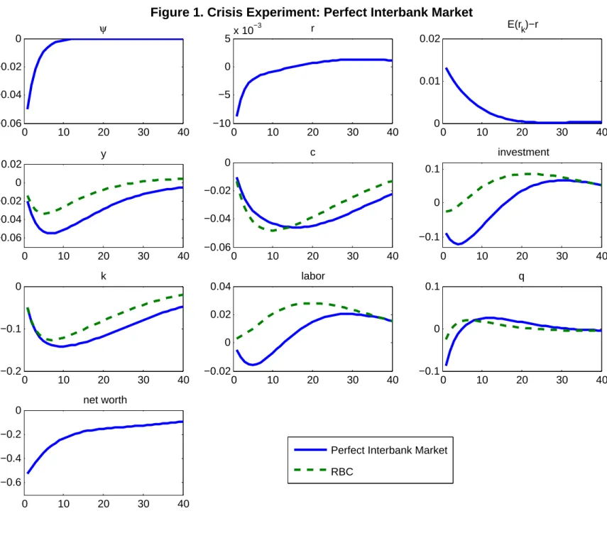
Absent credit market frictions, the model reduces to a real business cycle framework modified with habit formation and flow investment adjustment costs. With the credit market frictions, however, balance sheet constraints on banks ability to obtain funds in retail and wholesale market may limit real investment spending, affecting aggregate real activity. As we will show, a crisis is possible where weakening of bank balance sheets significantly disrupts credit flows, depressing real activity.
As we have discussed, one example of a factor that could weaken bank balance sheets is a deterioration of the underlying quality of capital. A negative quality shock directly reduces the value of bank net worth, forcing banks to reduce asset holdings. A second round effect on bank net worth arises as thefire sale of assets reduces the market price of capital. Further, the overall impact on bank equity of the decline in asset values is proportionate to the amount of bank leverage. With highly leveraged banks, a substantial percentage drop in bank equity may arise, leading to a significant disruption of credit flows. We illustrate this point clearly in section 4.
3
Credit Policies
During the crisis the various central banks, including the US. Federal Reserve, made use of their powers as a lender of last resort to facilitate creditflows. To justify such actions, the Fed appealed to Section 13.3 of the Federal Reserve Act, which permits it in "unusual end exigent circumstances" to make loans to the private sector, so long as the loans are judged to be of sufficiently high grade. The statute makes clear that in normal times the Fed is not permitted to take on private credit risk. In a crisis, however, the Fed has
freedom to fulfill its responsibility as lender of last resort, provided that it does not absorb undue risk.
In practice, the Fed employed three general types of credit policies. First, early on it expanded discount window operations by permitting discount window loans to be collateralized by high grade private securities and also by extending the availability of the window to non-bank financial institutions. Second, the Fed lent directly in high grade credit markets, funding assets that included commercial paper, agency debt and mortgage backed securities. Third, the Treasury, acting in concert with the Fed, injected equity in the banking system along with supplying bank debt guarantees (together with the Federal Deposit Insurance Corporation).
There is some evidence that these types of policies were effective in stabi-lizing thefinancial system. The expanded liquidity helped smoothed theflow of funds betweenfinancial institutions, effectively by dampening the turmoil-induced increases in the spread between the interbank lending rate (LIBOR) and the Treasury Bill rate. The enhanced financial distress following the Lehmann failure, however, proved to be too much for the liquidity facilities alone to handle. At this point, the Fed set up facilities to lend directly to the commercial paper market and a number of weeks later phased in programs to purchase agency debt and mortgage backed securities. Credit spreads in each these markets fell.
The equity injections also came soon after Lehmann. Though not with-out controversy, the equity injections appeared to reduce stress in banking markets. Upon the initial injection of equity in mid-October 2008, credit default swap rates of the major banks fell dramatically. At the time of this writing, the receiving banks have paid back a considerable portion of the funds. Further, though risks remain, the government appears to have made money on many of these programs.
In the sub-sections below, we take a first pass at analyzing how these policies work, using our baseline model.13 As we showed in the previous
section, within the context of our model, the financial market frictions open the possibility of periods of distress where excess returns on assets are ab-normally high. Because they are balance sheet constrained, private financial intermediaries cannot immediately arbitrage these returns. One can view the point of the Fed’s various credit programs as facilitating this arbitrage in
13For related attempts to model credit policy, see Curdia and Woodford (2009a, 2009b), Reis (2009), and Sargent and Wallace (1983).
times of crisis. In this regard, each of the various policies works somewhat differently, as we discuss below.
Before proceeding, we emphasize that, consistent with the Federal Reserve Act, we have in mind that these interventions be used only during crises and not during normal times. Indeed, within the logic of the model, the net benefits from credit policy are increasing in the distortion of credit markets that the crisis induces, as measured by the excess return on capital.
3.1
Lending Facilities (Direct Lending)
What we mean by direct lending is meant to broadly characterize the facilities the Fed set up for direct acquisition of high quality private securities.
Lending facilities work as follows: We suppose that the central bank has both an advantage and a disadvantage relative to private lenders. The ad-vantage is that unlike private intermediaries, the central bank is not balance sheet constrained (at least in the same way). Private citizens do not have to worry about the central bank defaulting. The liabilities it issues are gov-ernment debt and it can credibly commit to honoring this debt (aside from inflation). Thus, in periods of distress where private intermediaries are un-able to obtain additional funds, the central bank can obtain funds and then channel them to markets with abnormal excess returns.14
In the current crisis, the Fed funded the initial expansion of its lending programs by issuing government debt (that it borrowed from the Treasury) and then later made use of interest bearing reserves. The latter are effectively government debt. It is true that the interest rate on reserves fell to zero as the Federal Funds rate reached its lower bound, giving these reserves the appearance of money. However, once the Fed moves the Funds rate above zero it will also raise the interest rate on reserves. In this regard, the Fed’s unconventional policies should be thought of as expanded central interme-diation as opposed to expanding the money supply. In the case of lending facilities, a key advantage of the central bank is that it is not constrained in its ability to funds the same way as private intermediaries may be in time
14Others have also emphasized how that special nature of government liabilities can give rise to a productive role for governmentfinancial intermediations. See, example, Sargent and Wallace (1983), Kiyotaki and Moore (2008), Gertler and Karadi (2009), and Shleifer and Vishny (2010). As originally noted by Wallace (1980), unless there is something special about government liabilities, the Miller-Modigliani theorem applies to government finance.
of financial distress. Another equally important advantage is that the Fed can lend in many markets. By contrast, private banks face a limited market participation constraint, i.e., they can only lend to nonfinancial firms of the same island.
At the same time, we suppose that the central bank is less efficient at intermediating funds. It faces an efficiency cost τ per unit, which may be thought of as a cost of evaluating and monitoring borrowers that is above and beyond what a private intermediary (who has specific knowledge of a particular market) would pay.15
To obtain funds, the central bank issues government debt to the private that is a perfect substitute for bank deposits, and pays the riskless real rate Rt+1. It lends the funds in market h at the private loan rate Rhh
0
kt+1 which
depends upon the state of the next period h0. Observe that the central
banks is not offering the funds at a subsidized rate. However, by expanding the supply of funds available in the market, it will reduce equilibrium lending rates.
Let Sth be total securities of type h intermediated, Spth total securities
of type h intermediated by private banks, and Sh
gt total type h securities
intermediated by the central bank. Then total intermediation of type h assets is given by:
QhtSth =Qht(Spth +Sgth) (43) We suppose the central bank chooses to intermediate the fractionϕht of total
credit in market h: Sgth =ϕ h tS h t (44) where ϕh
t may be thought of as an instrument of central bank credit policy.
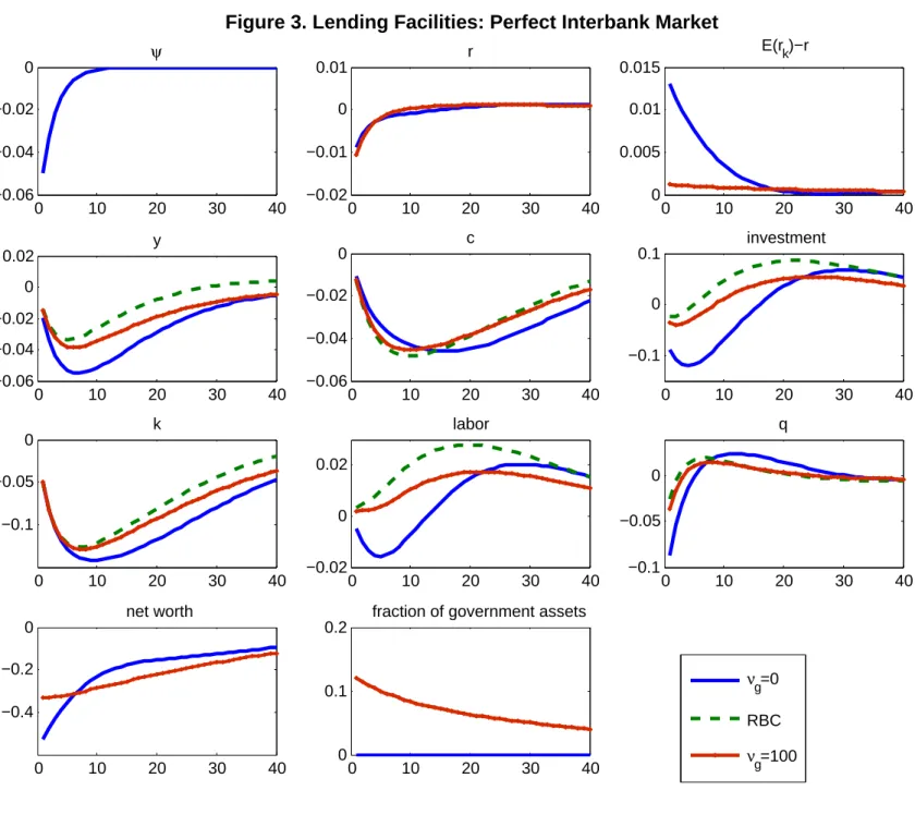
Assuming that banks investing regions are constrained under a symmetric frictions in wholesale and retail financial markets (ω = 0), lending facilities expand the total amount of assets intermediated in the market. Combining equations (31), (43) and (44), yields
QitSti = 1 1−ϕi
t
φitNti (45)
15Other potential costs include the potential for politicization of credit flows. We ab-stract from this consideration, though we think it provides another important reason for why credit policies are more appropriate in crises than normal times.
The effect on asset demand for non-investing regions depends on whether or not banks in these regions are balance sheet constrained (i.e., on whether the excess return μn
t > 0 is positive). If they are, then lending facilities
affect asset demands similarly to the way they do in investing regions, only the superscript i is replaced by n in (45). One other hand, if banks in non-investing regions are not constrained (i.e., μn
t = 0), then central bank
credit merely displaces private credit, leaving total asset demand in the sector unaffected. LetStn∗be total asset demand consistent with a zero excess return
on assets on non-investing islands in equilibrium. Then
QntStn∗ =QntSptn +ϕtnQntStn∗, iffμnt = 0. (46)
Here an increase in central credit provision crowds out private intermediation one for one. Only when private intermediaries are financially constrained does central bank intermediation expand the overall supply of credit.
3.2
Liquidity Facilities (Discount Window Lending)
With liquidity facilities, the central bank uses the discount window to lend funds to banks that in turn lend them out to nonfinancial borrowers. Typi-cally, liquidity facilitates are used to offset disruption of inter-bank markets. Such was the case in the current crisis.
Another distinguishing feature of liquidity facilities is that central bank lending is typically done at a penalty rate. This prescription dates back to Bagehot (1873). The idea is that during a liquidity crises, it is the breakdown of markets for short term funds that is responsible for many borrowers having limited credit access, as opposed to lack of credit worthiness of individual borrowers. Because excess returns for these borrowers are abnormally high during the crisis, they are more than willing to borrow at penalty rates. Offering the funds at a penalty rate, further, discourages inefficient use of central bank credit by the private sector.
In this section we use our model to illustrate how discount window lending may facilitate the flow of inter-bank lending during a crisis. To do so, we restrict attention to the case (ω = 0), where borrowers in the inter-bank market face symmetric constraints on obtaining funds in both the wholesale and retail markets. In this instance, banks with surplus funds face the same risk as depositors that borrowing banks may divert a fraction of gross assets for their own purposes.
We suppose the central bank offers discount window credit at the non-contingent interest rateRmt+1to banks who borrow on the inter-bank market.
It funds this activity by issuing government debt that is a perfect substitute for household deposits. For discount window lending to expand the supply of funds in the inter-bank market, however, the central bank must have an advantage over private lenders in supplying funds to borrowing banks. Otherwise discount window lending will simply supplant private inter-bank lending.
Here we suppose that the central bank is better able to enforce repay-ment than private lenders. In particular for any unit of discount window credit supplied, a borrowing bank can divert only the fraction θ(1−ωg) of
assets, with 0< ωg ≤ 1. Recall that for credit supplied by a private lender,
the borrowing bank can divert the fraction θ > θ(1−ωg). Here the idea is
that the government may have additional means at its disposal (IRS records, access to credit records, legal punishments, etc.) to retrieve assets. We suppose, however, that after a certain level of discount window lending, the central bank’s ability to retrieve assets more efficiently than the private sec-tor disappears. Think of this as reflecting some capacity constraint on the central bank’s ability to efficiently process discounted window loans secured by private credit.16
Letmh
t be discount window borrowing for a bank of typeh. The flow of
funds constraint is now,
Qhtsht =nht +bht +mht +dt. (47)
with mht ≥ 0. Let Vt(sht, bht, mht, dt) be the value of a bank who holds assets
and liabilities(sh
t, bht, mht, dt)at the end of periodt. For the bank to continue
operating this value must not fall below the gain from diverting assets, taking into account the central bank’s advantage in retrieving assets. Accordingly, in this case the incentive constraint is given by:
Vt(sht, b h t, m h t, dt)≥θ ¡ Qhtsht −ωgmht ¢ . (48)
16Alternatively, if we had asset heterogeneity this constraint might reflect a limitation on the kind of bank assets that might be suitable collateral for discount window lending. For example, information-intensive commercial and industrial loans are not good collateral for discount window loans since they require expertise for monitoring and evaluation. On the other hand, agency debt or high grade securitized mortgage might be suitable, but banks might only have a limited fraction in their portfolios.
We defer the details of the bank’s decision problem for this case to the Appendix. Accordingly, let μmt be the excess cost to a bank of discount
window credit relative to deposits μmt = Et
h0Λt,t+1Ω
h0
t+1(Rmt+1−Rt+1). (49)
Next note that, because we are restricting attention to the case of symmetric frictions in private interbank and retail financial markets (ω = 0), the inter-bank rate equals the deposit rate: Rbt+1 = Rt+1. Then from the first order
conditions we learn that in order for both private interbank borrowing and discount window to be actively used, we need:
μmt=ωgμit (50)
where μi
t is the excess value of assets on investing islands, given by equation
(30).
According to equation (50), to make borrowers indifferent between dis-count window and private credit at the margin, the central bank should set Rmt+1 to make the excess cost of discount window credit equal to the fraction
ωg of the excess value of assets. Intuitively, because a unit of discount
win-dow credit permits a borrowing bank to expand assets by a greater amount than a unit private interbank credit, it is willing to pay a higher cost for this form of credit. In this way, the model generates an endogenously determined penalty rate for discount window lending.
LetMt be the total supply of discount window credit offered to the
mar-ket. Then one can show that the market demand for assets by investing banks is given by QitS i pt =φ i tN i t +ωgMt. (51)
Thus, so long asωg >0, discount window lending can expand the total level
of assets intermediated by banks on investing regions.
Because the excess value of bank assets on non-investing islands is less than that on investing islands, i.e., μnt < μit., banks on non-investing islands
will not borrow from the discount window. Given that the discount rate is set to satisfy equation (50) discount window lending will be too expensive for banks who do not have new investment to finance.
The question then arises as to why the central bank does not simply expand discount lending to drive excess values of assets to zero. As we noted earlier, it reasonable to suppose that there are capacity constraints on
the central bank’s ability to adequately monitor bank’s asset management activities, (even though we do not formally incorporate it into our model here). With a capacity constraint on discount window lending (secured by private credit) the central bank may need to use other tools such as direct lending or equity injections during crisis periods of high excess returns. While liquidity facilities may be useful for improving theflow of funds in inter-bank markets, in a major crisis other kinds of interventions may be necessary to stabilize financial markets.
3.3
Equity Injections.
With equity injections, the fiscal authority coordinates with the monetary authority to acquire ownership positions in banks. As with direct central bank lending we suppose that there are efficiency costs associated with gov-ernment acquisition of equity. Let this cost beτeper unit of equity acquired.
During afinancial crisis, however, the net benefits from equity injections may be positive and significant.
The effect of equity injections depends on three factors: (i) the payout rule for government equity; (ii) the price at which the government acquires the equity relative to the market price; and (iii) the advantage the government might have relative to private creditors in addressing the agency problem with banks.
The government injects equity into banks who stay active (instead of exiting) at the beginning of period before banks learn whether their customers have opportunities to invest or not. This is different from the direct lending and discount window lending activities of the central bank that are conducted after the arrival of investment opportunities. By this difference in timing, we try to capture a feature that the equity injections are slower than the direct lending and discount window lending. For simplicity we restrict attention to the case with a perfect interbank market in which banks cannot divert assets that are financed by interbank borrowing. (See the Appendix for a general case). Then the asset price is equal across regions with different investment opportunity.
We suppose that a unit of government equity has the same payout stream as a unit of private equity. The government may hold the equity stake until the bank exits and then receive the liquidation value of its assets, equal to
Zτ + (1−δ)Qτ per unit of capital times the number of units of capital its
shares are worth. Alternatively it may sell offits holding at this value before the bank exits, assuming the crisis has passed.
Accordingly, one can effectively divide the total number of securities held by the bank at timet between those privately owned,spt, and those publicly
owned, sget:
st=spt+sget (52)
Letngt be the market value of government equity. The bank’s balance sheet
identity then implies:
Qtst=nt+bt+dt+ngt (53)
where each security the government holds is valued at the market price Qt,
implying:
ngt=Qtsget (54)
To acquire equity, the government may pay a price Qgt that is above
Qt. One rationale for the government paying a premium is that the market
price is below its normal value due to financial distress. For example, the government could pick Qgt so that the excess return on government equity,
μgt, equals zero, as follows:
μgt=EtΛt,t+1Ωt+1(Rgkt+1−Rt+1) (55)
where Rgkt+1 is the gross return on a unit of government equity injected at
time t is:
Rgkt+1 =ψt+1
Zt+1+ (1−δ)Qt+1
Qgt
(56) Since the excess return of private equity is positive (see equation (22)),Qgt>
Qt.
The premium the government pays for equity is effectively a transfer to the bank that shows up in its net worth as follows:
nt= [Zt+(1−δ)Qt]ψtspt−1−Rbtbt−1−Rtdt−1+(Qgt−Qt)[sget−(1−δ)ψtsget−1]
(57) where (Qgt−Qt)(sgt−sgt−1) is the "gift" to the bank from new government
We suppose that the bank cannot divert assets financed by government equity. As with discount window lending, the government has an advan-tage relative to the private creditors in recovering assets. Accordingly, the incentive constraint becomes,
Vt(st−sget, bt, dt)≥θ(Qt(st−sget)−bt).
where as before bt is interbank borrowing (withω = 1).
Let Ngt be total government equity in the banking system and Sgt be
total holdings of government equity. Then we can aggregate to obtain the following expressions for aggregate asset demand and for the evolution of net worth:
QtSt=φtNt+Ngt (58)
Nt = (σ+ξ)[Zt+(1−δ)Qt]ψtSpt−1−σRtDt−1+(Qgt−Qt)[Sget−(1−δ)ψtSget−1]
(59) where φt is the leverage ratio privately intermediated assets in the case of a
perfect inter-bank market (see equation (20)), and with Ngt =QtSget. Thus,
in this case equity injections expand the value of assets intermediated one-for-one, as equation (58) suggests. In addition, to the extent the government paying pays a premium over the market price (which is depressed due to the
financial crisis), the equity injection also expands private bank net worth, as equation (59) indicates. This is in turn expands asset demand by a multiple equal to the leverage ratio φt.
One additional important effect of government equity injections is they reduce the impact of unanticipated changes in asset values on private bank equity. Absent government equity, for example, the bank absorbs entirely the loss from an unanticipated decline in asset values, given that its obligations to outsiders are all in the form of non-contingent debt. With public equity, however, the government shares proportionately in the loss.
A key question now is what might determine the allocation of credit pol-icy intervention between direct lending, discount window lending and equity injections. We argued earlier that in the context of our model, it might be natural to think of capacity constraints on discount window lending secured by private credit. So long as the efficiency costs of direct central bank lend-ing are not large, extensive use of the direct lendlend-ing makes sense. For high grade instruments like commercial paper, agency debt and mortgage backed securities it is reasonable to suppose the costs of central bank intermediation are not large. This might account for why direct central bank lending in the