Generating Diagnoses for
Probabilistic Model Checking
Using Causality
Hichem Debbi and Mustapha Bourahla
Department of Computer Science, University of M’sila, Algeria
One of the major advantages of model checking over other formal methods of verification is its ability to generate an error trace when the specification is falsified in the model. We call this trace a counterexample. In probabilistic model checking(PMC), counterexample generation has a quantitative aspect. The counterexample is a set of paths in which a path formula holds, and their accumulated probability mass violates the probability bound. In this paper, we address the complementary task of counterexample generation, which is the coun-terexample diagnosis. We propose an aided-diagnostic method for probabilistic counterexamples based on the notion of causality. Given a counterexample for a probabilistic CTL (PCTL) formula that does not hold over Discrete Time Markov Chain(DTMC)model, this method guides the user to the most responsible causes in the counterexample.
Keywords: Discrete-Time Markov Chain(DTMC), Prob-abilistic Model Checking(PMC), Probabilistic Computa-tion Tree Logic(PCTL), Probabilistic Counterexamples, Causality
1. Introduction
Probabilistic model checking has appeared as an extension of model checking for modeling and analyzing systems that exhibit stochastic behavior. Several case studies in several do-mains have been addressed from randomized distributed algorithms and network protocols to biological systems and cloud computing envi-ronments. These systems are described usually using Discrete-Time Markov Chains(DTMC), Continuous-Time Markov Chains (CTMC) or Markov Decision Processes (MDP), and veri-fied against properties speciveri-fied in Probabilistic Computation Tree Logic (PCTL) [24] or Con-tinuous Stochastic Logic(CSL) [7, 8].
For counterexample generation in probabilistic model checking(PMC), many approaches have been proposed. But unlike the previous method proposed for conventional model checking that generates the counterexample as a single path ending with a bad state representing the failure
[14], the task in PMC is quite different. The counterexample in PMC is a set of evidences or diagnostic paths that satisfy the formula and their probability mass violates the probability bound. As it is in conventional model checking, the generated counterexample should be small and indicative to be easy for analyzing[4, 22].
However, generating small and indicative coun-terexamples only is not enough for understand-ing the error. Therefore, many works in con-ventional model checking have addressed the analysis of counterexamples to better under-stand the error [9, 19, 20, 28, 38 and 40]. As it was done in conventional model checking, addressing the error explanation in the proba-bilistic model checking is highly required, es-pecially that probabilistic counterexample con-sists of multiple paths instead of single path, and that it is probabilistic.
based on them. Our approach for error expla-nation is based on the smallest most indicative counterexamples[4, 22]. To our knowledge, no work has been done yet for error explanation in probabilistic model checking.
The rest of this paper is organized as follows. In Section 2, we present some preliminaries and definitions. The probabilistic logic PCTL and probabilistic counterexamples are presented in this section. In Section 3, we give the def-inition of causes in probabilistic counterexam-ples with the formal causality model. Following that, we introduce an algorithm for generating the causes and their responsibilities for the vio-lation of PCTL properties. Experimental results are given in Section 5. Section 6 presents the re-lated works. At the end, we present conclusion and future works.
2. Preliminaries and Definitions
We call a discrete-time stochastic process with discrete state space a Discrete-Time Markov Chain(DTMC)if it satisfies the Markov prop-erty:
P[xn =in|x0=i0,x1 =i1, . . . ,xn−1 =in−1]
=P[xn=in|xn−1=in−1]
This means, the probability to pass to next state depends only on the previous state and not on the state’s history.
More formally, a DTMC is a tupleD= (S,sinit,
P,L), such thatSis a finite set of states,sinit∈S the initial state, P : S×S → [0,1] represents the transition probability matrix, L : S → 2AP is a labelling function that assigns to each state
s ∈ S the setL(s) of atomic propositions. An infinite pathσis a sequence of statess0s1s2. . ., where P(si,si+1) > 0 for all i ≥ 0. A finite path is finite prefix of an infinite path. We de-fine a set of paths starting from a state s0 by
Paths(s0). The underlyingσ-algebra is formed by the cylinder sets which are induced by fi-nite paths inPaths(s0). The probability of this cylinder set is:
P(σ ∈Paths(s0)|s0s1. . .snis a prefix ofσ)
=
i≤0<n
P(si,si+1)
2.1. Probabilistic Computation Tree Logic (PCTL)
The Probabilistic Computation Tree Logic
(PCTL)has appeared as an extension of CTL for the specification of systems that exhibit stochas-tic behaviour. We use the PCTL for defining quantitative properties of DTMCs. PCTL state formulas are formed according to the following grammar:
φ ::=true|a|¬φ|φ1∧φ2|P∼p(ϕ)
Wherea∈ APis an atomic proposition,ϕ is a path formula,Pis a probability threshold opera-tor,∼∈ {<,≤, >,≥}is a comparison operator, andp is a probability threshold. The path for-mulasϕare formed according to the following grammar:
ϕ ::=φ1Uφ2|φ1Wφ2|φ1U≤nφ2|φ1W≤nφ2 Where φ1 and φ2 are state formulas and n ∈
N. As in CTL, the temporal operators (U for strong until,Wfor weak(unless)until and their bounded variants) are required to be immedi-ately preceded by the threshold operatorP.The PCTL formula is a state formula, where path formulas occur only inside the operatorP. The operatorPcan be seen as a quantification oper-ator for both the operoper-ators∀(universal quantifi-cation)and∃(existential quantification), since the properties are representing quantitative re-quirements.
The semantics of a PCTL state formulaφ over a state s (or a path σ) in a DTMC model
D= (S,sinit,P,L)can be defined by a satisfac-tion relasatisfac-tion denoted by|=. A pathσ =s0s1. . . satisfies a PCTL formulaφif the relations0|=φ is satisfied. We define the set of paths satisfy-ing the relations|=φ byPaths(s|=φ)and the probability of the satisfaction ofs|=φ by
P(s|=φ) =
σ∈Paths(s|=φ)P(σ)
The PCTL semantics is defined as follows:
s|=true⇔true s|=a⇔a∈L(s) s|=¬φ ⇔s|=φ
s|=φ1∧φ2 ⇔s|=φ1∧s|=φ2
σ |=φ1Uφ2⇔ ∃j≥0.σ[j]
|=φ2∧(∀0≤k<j.σ[k]|=φ1)
σ |=φ1Wφ2⇔σ |=φ1Uφ2
∨(∀k ≥0.σ[k]|=φ1)
σ |=φ1U≤nφ2⇔ ∃0≤j≤n.σ[j]
|=φ2∧(∀0≤k<j.σ[k]|=φ1)
σ |=φ1W≤nφ2⇔σ |=φ1U≤nφ2
∨(∀0≤k ≤n.σ[k]|=φ1)
In the rest of the paper, we will focus on prop-erties of upper probability bound of the form
φ1Uφ2 or its variant (φ1U≤nφ2). Probabilistic lower bounded properties can be easily trans-formed to upper bounded properties[4, 22].
2.2. Probabilistic Counterexamples
The probabilistic counterexamples are gener-ated when a PCTL property is not satisfied. The probabilistic property φ = P≤p(ϕ) is refuted when the probability mass of the paths satisfy-ingϕ exceeds the boundp. Therefore, a prob-abilistic counterexample for the propertyφ can be formed of a set of finite paths starting at state
sand satisfying the path formulaϕ. We refer to these paths as FinitePaths(s|=φ). Thus, each path σ = s0s1. . .sn from FinitePaths(s |= φ) is a prefix of an infinite path fromPaths(s|=φ)
satisfying the formula φ. FinitePaths(s |= φ)
are also called diagnostic paths[4, 5].
It is clear that we can get a set of probabilistic counterexamples, notedPCX(s |=φ), which is a set of any combination fromFinitePaths(s|=
φ), their probability mass exceeds the boundp. Among all these probabilistic counterexamples, we are interested by the most indicative one. The most indicative counterexample is minimal counterexample(has the least number of paths from FinitePaths(s |= φ)) and its probability mass is the highest among all other minimal counterexamples. We denote the most indica-tive probabilistic counterexample byMIPCX(s0
|= φ). We should note that the most indica-tive probabilistic counterexample may not be unique.
Lemma 2.1 LetMIPCX(s0 |= φ)be the most indicative probabilistic counterexample. Every finite path σ ∈ MIPCX(s0 |= φ) is critical.
Which means ∀σ : MIPCX(s0 |= φ)−σ ( re-moving any pathσfromMIPCX(s0 |=φ))will render the result not a counterexample.
For the counterexample to have high probabil-ity, it should consist of paths that carry high probabilities from FinitePaths(s |= φ). The path σ having the highest probability over all these paths is called the strongest path and is defined as follows: for every path σ ∈ FinitePaths(s |= φ) : P(σ) ≥ P(σ). The
strongest path also may not be unique.
Lemma 2.2 The most indicative probabilistic counterexample contains at least one strongest pathσ ∈FinitePaths(s|=φ).
Corollary 2.1If a path propertyφ1Uφ2(φ1U≤n
φ2)is satisfied in a finite path σ, the right state sub-formula(φ2)is satisfied in the last state of
σ.
Lemma 2.3 According to the semantics pre-sented above, any PCTL path formula, if it is satisfied on a finite path, it is also satisfied on any suffix of this path.
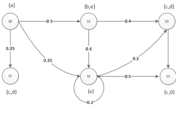
Example 2.1 Let us consider the example of DTMC shown in Figure 1 and the property
P≤0.5(ϕ), whereϕ = (a∨b)U(c∧d).
Figure 1.A DTMC.
The property above is violated in this model
(s0 |=P≤0.5(ϕ)), since the probability mass of all paths satisfying ϕ is higher than the proba-bility bound(0.5). We have
FinitePaths(s0|=φ) =
{s0s1,s0s2s3,s0s2s4s3,s0s2s4s5,s0s4s5} Any combination of paths fromFinitePaths(s0
is a valid probabilistic counterexample includ-ing the whole set. For instance, we can find three counterexamples:
P(C1)=P({s0s1,s0s2s3,s0s2s4s3,s0s2s4s5,s0s4s5)
=0.25+0.2+0.09+0.15+0.12=0.81
P(C2) =P({s0s1,s0s2s4s5,s0s4s5})
=0.25+0.15+0.12=0.52
P(C3) =P({s0s1,s0s2s3,s0s2s4s5})
=0.25+0.2+0.15=0.60
The last probabilistic counterexample is the most indicative one, since it is minimal and its probability is higher than the other minimal counterexample C2, P(C3) = 0.6 > P(C2). The strongest path iss0s1, which is included in the most indicative probabilistic counterexam-ple.
3. Causes in Probabilistic Counterexamples
For PCTL properties of the form φ = P≤p(ϕ), explaining the violation reduces to the expla-nation of exceeding the probability bound over the DTMC model. Therefore, the question of “what labelling and/or probability values in the counterexample cause the system to falsify a specification” reduces to the question: “what labelling and/or probability values in the coun-terexample cause the exceeding of probability bound over the model”.
3.1. Causality Model
The counterfactual notion of causality[30]states that: event A is a cause of event B if, had A not happened, then B would not have happened. Unfortunately, this statement does not cover all real cases. Let’s take the major known exam-ple of Suzy and Billy who both pick up rocks and throw them at a bottle [21]. Suzy’s rock gets there first, shattering the bottle. Since both throws are perfectly accurate, Billy’s would have shattered the bottle had it not been pre-empted by Suzy’s throw. Thus, according to the counterfactual condition, Suzy’s throw is not a cause for shattering the bottle. Halpern and Pearl[21]have addressed this issue by tak-ing A to be a cause of B if B counterfactually
depends on A under some contingency. For example, Suzy’s throw is a cause of the bottle shattering because the bottle shattering coun-terfactually depends on Suzy’s throw, under the contingency that Billy does not throw.
With respect to the definition of causality by Halpern and Pearl [21], the causality model
M is defined by a set of exogenous variables
U, whose values −→u are determined by factors outside the model M, but they should be rep-resented to encode the context, and by a set of endogenous variables V, whose values are determined by structural equations, and set of functions F, where each fvi ∈ F is a mapping
from U ×(V \Vi) to Vi. Thus, each fvi tells
us the value ofVi given the values of all other variables inU∪V. The causality model M has no control on context changes.
We can define a causality model for the most indicative counterexampleMIPCX(s0 |=φ)as a tupleM= (U,V,F), whereUis presented by a single variable; we call it a context variable, its valueuencodes a state inMIPCX(s0 |= φ). V is a set of variables representing atomic propo-sitions and Boolean formulas. F is a set of truth functions associating to every variable in V a value (0 or 1). So, each fvi ∈ F tells
us the value of a variable in V given the val-ues of all the other variables. For example,
fp∧r(s,p = 1,r = 1) = 1 where p and r are atomic propositions, andsis state representing a context. The causal influences in are modelled by the transitions inMIPCX(s0|=φ).
3.2. Generating Causes
We call the path until formula ϕ a causal for-mula. We write (M,u) |= ϕ if ϕ is true in causality modelMgiven a contextu. We write
(M,u) |= [−→Y ← −→y ](X = x), ifX has a value
(0or1) in M given a context u and the assign-ment−→y to−→Y , where−→Y ⊂V.
We write (M,u) |= ϕ if ϕ is true in causal-ity model given a contextu. For probabilistic causality, we add a probability to each context, which is a statesbelonging to finite paths from
Therefore, a context probability is defined by this equation:
P(u=s) =
s∈σ|σ∈MIPCX(s0|=φ)
P(σ)
The statement for causality is “A formula Cis a cause of ϕ in contextu ofM”. The types of formulas that are allowed to be causes forϕare ones of the form X1 = x1 ∧ . . .∧ Xk = xk which is abbreviated to the form −→X = −→x . Since F defines a mapping from U to V, We can associate to each cause a probability that represents exactly the context probability as
P(−→X =−→x ) =P(s).
With all these definitions in hand, we can now give the definition of an actual cause for the violation of PCTL propertyφ =P≤p(ϕ).
Definition 3.1we say that−→X =−→x is an actual cause for the violation ofφ =P≤p(ϕ)in(M,s) with a probability equal toP(−→X =−→x ) =P(s)
if the following holds:
1. (M,s)|= (−→X =−→x )∧ϕ
2. There exists a partition (−→Z,−→W) of V with
−→X ⊆ −→Z and some setting(−→x ,−→w)of the
variables in(−→X,−→W)such that if(M,s)|= Z =zforZ ∈ −→Z then
(M,s)|=−→X ← −→x,−→W ← −→w∧ ¬ϕ
and(M,s)|=−→X ← −→x ,−→W ← −→w,
−→Z ← −→z ∧ϕ for all subsets−→Z of−→Z.
3. The set of variables−→X is minimal(no subset of−→X satisfies the conditions 1 and 2).
The first condition states that both −→X = −→x
andϕ are true in the current context, given the variables −→X and their values −→x . The second condition states that any change on(−→X,−→W)will change ϕ from true to false, changing −→W will have no effect onϕ as long as the values of−→X
are kept at the current values, even if all subsets
−→Z of−→Z are set to their original values in the
current context. Minimality condition ensures
that only elements in the conjunction−→X = −→x
are essential for changingϕ from true to false. Each cause X = x has a probabilityP(X = x)
that measures its contribution to the error, where the cause involved in the satisfaction of ϕ in more paths is usually the most probable cause. So that, given the probability ofMIPCX(s0 |=
φ), we associate to each cause a degree of con-tribution for the error, and we call it responsibil-ity. The degree of responsibility of each cause is given by:
R(X =x) =P(X=x)/P(MIPCX(s0|=φ))
Definition 3.2 A causeC1 has more responsi-bility over another causeC2for the violation of
φ =P≤p(ϕ), ifR(C1)>R(C2).
Example 3.1Consider the most indicative coun-terexample C3 = {s0s1,s0s2s3,s0s2s4s5} gen-erated from the DTMC presented in Figure 1 against the propertyP≤0.5[(a∨b)U(c∧d)]. It is possible to define a causality model forC3, where u ∈ {s0,s1,s2,s3,s4,s5}, and F can be defined over the variables inV as follows
fb(s2) =1
fc∧d(s2,c=0,d =0) =0 ...
For instance, it is clear that in s2,−→X = {b},
−→Z = {b,e} and −→W = {a,c,d}. So, the
cause in s2 is b = 1 with a responsibility
R(b=1) = (0.2+0.15)/0.6=0.58.
4. Algorithm for Generating Causes
formulaϕis until formula written in NNF( Neg-ative Normal Form), which means that negation appears just at the front of atomic propositions.
Algorithm. GenerateCauses
Inputs: The most indicative counterexample
MIPCX(s0|=φ)
The probabilistic formulaφ =P≤p(ϕ)whereϕ is of
the formφ1Uφ2or(φ1U≤nφ2)
Outputs: Set of causes with their responsibili-ties
Begin
Contexts :=ComputeContexts(MIPCX(s0|=φ)) Causes :=∅
Foreach contextsfrom the contexts set
Ifsis the last state in a pathσ then
Causes :=Causes∪FindCauses(s,φ2) R(Causes)=s∈σ|σ∈MIPCX(s0|=φ)P(σ)/
P(MIPCX(s0|=φ))
End If Else
Causes :=Causes∪FindCauses(s,φ1) R(Causes)=s∈σ|σ∈MIPCX(s0|=φ)P(σ)/
P(MIPCX(s0|=φ))
End Else End For Sort(Causes)
End GenerateCauses Function FindCauses(s,ψ)
Begin
Ifψis of the formawherea∈APanda∈L(s)
Thenreturns,a
End If
If ψ is of the form ¬a where a ∈ AP and
a∈/ L(s)
Thenreturns,¬a
End If
Ifψ is of the formψ1∧ψ2Then return{FindCauses(s,ψ1)∪
FindCauses(s,ψ2)}
End If
Ifψ is of the formψ1∨ψ2Then return{FindCauses(s,ψ1)} ∪
{FindCauses(s,ψ2)}
End If
Otherwise return∅ End FindCauses
The algorithm explores the counterexample and computes the causes and their responsibilities with respect to each state s. The causes then
will be sorted in order according to their respon-sibilitiesR. The main function of this algorithm is FindCauses, which is based on the formula structure. It takes a state and state formula as input and returns recursively the set of causes. The condition put on the last state follows Corol-lary 2.1. We note that when the state formula
ψ is of the form ψ1 ∧ψ2, both sub-formulas are essentially true at state s. But when ψ is of the formψ1∨ψ2, one of them could be true ats or both of them. This actually follows the causal intuition that in the conjunctive scenario, both ψ1and ψ2 are required for ψ being satis-fied. Whereas in the disjunctive scenario, either
ψ1 or ψ2 suffices to make ψ satisfied. In the two cases, we apply FindCauses to each sub-formula. Finally, at the propositional level, the cause will be a pairs,a ifa∈L(s)ors,¬a
otherwise.
This algorithm computes an approximate set of causes, since computing the set of causes ex-actly in binary causal models is NP-complete
[16]. The reduction from binary causal models to Boolean circuits and from Boolean circuits to model checking as introduced in[12]proved that computing a set of causes for branching time formula can be done in linear time. There-fore, further analysis of the complexity of causes computing is beyond the scope of this paper.
5. Experimental Results
We have implemented the above method in Java. To evaluate our method, we use a bench-mark case study of the embedded control sys-tem taken from[31]. The system is modelled in prism as a CTMC[41]. We should mention that before performing the verification, the CTMC has to be transformed to its embedded DTMC. The system consists of input processor(I)that reads incoming data from three sensors(s1, s2 and s3) and then passes it to main processor
(M). The processor M processes the data and sends instructions to an output processor (O) that controls two actuators (A1 and A2)using these instructions. Any of the system’s compo-nents M, I/O, the sensors and the actuators may fail; as a result, the system is shut down. The types of failures are:
fail io = (count =MAX COUNT+1) fail main= (m=0)
We use the variable Max Count to refer to the maximum number of consecutive cycles skipped allowed. Thus, the I/O processor will fail if the count exceeds the limit Max Count. The down status of the system is labelled as:
down =fail sensors|fail actuators|fail io| fail main
For this model, we choose the PCTL property that estimates the probability of I/O failure oc-curring first, which is given as follows:
P=?[!(down)Ufail io]
We test this property using prism for(Max Count = 1). For this value, prism renders a probabil-ity equal to 0.43. We chose the value 0.4 as a threshold for this property to generate the coun-terexample. Thus the property can be rewritten as follows:
P≤0.4[!(down)Ufail io]
We use DiPro to generate the counterexample, which in turn uses prism. The counterexample rendered by DiPro can be saved in text format as well as in XML format. The tool imple-ments many algorithms. In our experiimple-ments, we used its heuristic search algorithm XBF that generates the sub-graph inducing the counterex-ample. Our method takes the counterexample generated from DiPro in XML format and the property to be verified as arguments, and out-puts the causes with their responsibilities. All the experiments were carried out on windows XP with Intel Pentium CPU 3.2 GHz speed and 512 mb of memory.
The prism model consists of 2633 states and 11072 transitions. For generating the coun-terexample, DiPro Explored 480 traces, 558 vertices and 1080 edges in more than 1 minute. Finally, the counterexample rendered consists of just 35 diagnostic paths. It is evident that the number of explored vertices and explored edges while searching the counterexample is less than the number of states and the transitions of the model. It is evident also that the number of diagnostic paths is less than the number of solution traces. While solution traces refer to
all the paths of the diagnostic sub-graph found through exploring the model, diagnostic paths refer just to the paths forming the counterexam-pleMIPCX(s0 |= φ). We pass this counterex-ample to our algorithm for generating the causes and their responsibilities. Our algorithm takes less than 1 second for generating the causes with their responsibilities. We notice that this time is negligible comparing to the size of the model and the time taken for computing the counterex-ample.
The causes generated are the basic sub-formulas satisfying the path formula ¬(down)Ufail io. For the right sub-formula (fail io), the cause generated isC0 = (count = MAX COUNT+
1). For the left sub-formula, the set of causes for the system not to be in down state is:
C1=¬(i=2),
C2=¬(s<MIN SENSORS) C3=¬(o=2),
C4=¬(a<MIN ACTUATORS) C5=¬(count=MAX COUNT+1) C6=¬(m=0)
C1and C2 refer to the probable causes for the failure in the level of sensors, whereasC3 and
case for actuators failure withC3 andC4. In all states,C2(all sensors are working)andC4(all actuators are working) are found to be the ac-tual causes of the absence of both, sensors and actuators failures. Thus, they have absolutely more responsibility than the two other causes in such states: C1 (input processor not Ok) and
C3(output processor not OK), respectively.
6. Related Works
The original algorithm for counterexample gen-eration was proposed by Clarke et al. [14]
and was implemented in most symbolic model checkers. This algorithm of generating lin-ear counterexamples for a fragment of ACTL
(ACTL∩LTL)was later extended to handle ar-bitrary ACTL properties [15] using the notion of tree-like counterexamples. Since then, many works have addressed this issue in conventional model checking[10, 18, 32, 36 and 37].
However, the counterexample generated does not indicate where the failure really exists. There-fore, counterexamples analysis is inevitable. In conventional model checking, many works have proposed techniques for discovering error causes from counterexamples, hence present-ing them to the user in a comprehensive way. Most of these works range in the software model checking and programs debugging, especially C programs, in the aim to find bugs in the source code[9, 19, 20 and 40]. Based on Lewis coun-terfactual theory of causality [30]and distance metrics, Groce et al. in [20] have proposed semi-automated approach for isolating errors in ANSI C programs by considering the alternative worlds as programs executions and the events as propositions about those executions. Unlike the previous work that requires multiple executions, the work[38]introduced a technique performed on a single concrete execution path using the weakest pre condition algorithm. While all of these works addressed safety properties, some of them attempted to explain errors for liveness properties, which involves more computational complexity[28].
For counterexample generation in probabilistic model checking(PMC), many approaches have been proposed. In [1,2], Aljazzar et al. intro-duced an approach for counterexample genera-tion for DTMC and CTMC against timed
reach-ability properties using heuristics guided and directed explicit state space search. In comple-mentary work [3], with the intuition that sin-gle scheduler makes an MDP as DTMC, they proposed an approach for counterexample gen-eration for MDPs using existing methods for DTMC. They introduced more complete work in[4]for generating counterexample for DTMC and CTMS as what they refer to as diagnostic sub-graphs. Based on all the previous works, they built an open source tool, DiPro [5], for generating counterexamples for DTMC, CTMC and MDPs. This tool can be used with the prob-abilistic model checkers PRISM and MRMC and renders the counterexamples graphically. Similar to the previous works, Han et al. have proposed the notion of the smallest most indica-tive counterexample that reduces to the problem of finding K shortest paths[22, 23]. Instead of generating path-based counterexamples, Wim-mer et al. have proposed a novel approach based on critical subsystems [39]. Following this work, the authors in[34]proposed the COMICS tool for generating the critical subsystems that induce the counterexamples. In[6], the authors proposed an approach for finding sets of evi-dences for bounded probabilistic LTL proper-ties on Markov Decision Processes(MDP)that behave differently from each other giving sig-nificant diagnostic information. More special cases are treated in[25, 33 and 35].
7. Conclusion and Future Works
In this paper, we have shown how the notion of causality can be interpreted in the context of probabilistic counterexamples. Due to the probabilistic nature of the causal model, we had to define for each context its probability. Accordingly, we defined for each cause its re-sponsibility that measures its contribution to the error inherited from the context it is located in. Following that, we introduced an algorithm for diagnoses generation that acts as a guided-method to the most responsible causes in the counterexample. The most responsible cause is considered to be the most relevant to the user. Evidently, our approach does not ignore the pre-vious works of counterexample generation, but instead, it acts as a complementary task. To our knowledge, we are the first who introduce di-agnosis approach that acts on counterexamples generated in PMC.
As future works, we aim to show how our method can also perform on counterexamples generated from CTMCs against CSL properties, as well as MDPs models. In this paper, we did not introduce a graphical way for representing the causes and their responsibilities, so as a fu-ture work, we aim to build a tool for generating the diagnoses graphically.
References
[1] H. ALJAZZAR, H. HERMANNS, S. LEUE,
Counterex-amples for timed probabilistic reachability. In For-mal Modeling and Analysis of Times systems (FOR-MATS),(2005), pp. 177–195.
[2] H. ALJAZZAR, S. LEUE, Extended directed search
for probabilistic timed reachability. InFORMATS,
(2006), pp. 33–51.
[3] H. ALJAZZAR, S. LEUE, Generation of
Counterexam-ples for Model Checking of Markov Decision Pro-cesses. InProceedings of the International Confer-ence on Quantitative Evaluation of Systems (QEST),
(2009), pp. 197–206.
[4] H. ALJAZZAR, S. LEUE, Directed explicit state-space
search in the generation of counterexamples for stochastic model checking. IEEE Trans. on Soft-ware Engineering, vol. 36 no. 1(2010), pp. 37–60.
[5] H. ALJAZZAR, S. LEUE, DiPro – A Tool f or
Proba-bilistic Counterexample Generation.LNCS,(2011), pp. 183–187. Available at http://www.inf.uni-konstanz.de/soft/dipro/
[6] M. E. ANDRES´ , P. R. D’ARGENIO, P.VANROSSUM, Significant Diagnostic Counterexamples in Prob-abilistic Model Checking. In Haifa Verification Conference,(2008), pp. 129–148.
[7] A. AZIZ, K. SANWAL, V. SINGHAL, R. BRAYTON, Model-checking continuous-time Markov chains.
ACM Transactions on Computational Logic, vol. 1, no. 1(2000), pp. 162–170.
[8] C. BAIER, B. HAVERKORT, H. HERMANNS, J.-P. KA -TOEN, Model checking algorithms for continuous-time Markov chains.IEEE Transactions on Software Engineering, vol. 29, no. 7(2003).
[9] T. BALL, M. NAIK, S. K. RAJAMANI, From symp-tom to cause: localizing errors in counterexample traces. InSymposium on Principles of Programing Languages (POPL),(2003), pp. 97–105.
[10] M. CHECHIK, A. GURFINKEL, A framework for
counterexample generation and exploration. In Fun-damentals Approaches to Software Engineering (FASE),(2005), pp. 217–233.
[11] H. CHOCKLER, I. BEER, S. BEN-DAVID, A. ORNI,
R. TREFLER, Explaining counterexamples using
causality. InBouajjani, A., Maler, O. (eds.), LNCS, vol. 5643(2009), pp. 94–108.
[12] H. CHOCKLER, J. Y. HALPERN, O. KUPFERMAN,
What causes a system to satisfy a specification?
ACM Transactions on Computational Logicvol. 9, no. 3(2007), pp. 1–24.
[13] H. CHOCKLER, J. Y. HALPERN, Responsibility and
blame: a structural-model approach.Journal of Ar-tificial Intelligence Research (JAIR), vol. 22(2004), pp. 93–115.
[14] E. CLARKE, O. GRUMBERG, M. C. MILLAN, X.
ZHAO, Efficient generation of counterexamples and witnesses in symbolic model checking. In Proceed-ings of the Design Automation Conference,(1995), pp. 427–432.
[15] E. CLARKE, Y. LU, S. JHA, H. VEITH, Tree-like
counterexamples in model checking. In Proceed-ings of the 17th Annual IEEE Symposium on Logic in Computer Science,(2002), pp. 19–29.
[16] T. EITER, T. LUKASIEWICZ, Complexity results for structure-based causality.Artificial Intelligence, vol. 142(2002), pp. 53–89, Elsevier.
[17] F. FISCHERS. LEUE, Causality Checking for
Com-plex System Models. InProceedings of the VMCAI, LNCS, vol. 7737(2013), pp. 248–276.
[18] P. GASTIN, P. MORO, Minimal counterexample
gen-eration for SPIN.LNCS, Vol. 4595(2007), Springer.
[19] A. GROCE, W. VISSER, What went wrong: explain-ing counterexamples. In Ball, T., Rajamani, S.K. (eds.) SPIN, LNCS, vol. 2648(2003), pp. 121–135.
[21] J. HALPERN, J. PEARL, Causes and explanations: A structural-model approach – part I: Causes. In
Proceedings of the 17th UAI,(2001), pp. 194–202.
[22] T. HAN, J. P. KATOEN, Counterexamples in proba-bilistic model checking. InTools and Algorithms for the Construction and Analysis of Systems (TACAS),
(2007).
[23] T. HAN, Diagnosis, synthesis and analysis of prob-abilistic models. Ph.D. Thesis, RWTH Aachen University, University of Twenty, 2009.
[24] H. HANSSON, B. JONSSON, Logic for reasoning
about time and reliability.Formal aspects of Com-puting, vol. 6, no. 5(1994), pp. 512–535.
[25] H. HERMANNS, B. WACHTER, L. ZHANG,
Probabilis-tic CEGAR. InProceedings of the Computer Aided Verification (CAV), LNCS, vol. 5123 (2008), pp. 162–175.
[26] A. HINTON, M. KWIATKOWSKA, G. NORMAN, D.
PARKER, PRISM: A tool for automatic
verifica-tion of probabilistic systems. InProceedings of the TACAS’06, vol. 3920(2006), pp. 441–444.
[27] J.-P. KATOEN, M. KHATTRI, I. S. ZAPREEV, A Markov Reward Model Checker. InQEST,(2005), pp. 243–244.
[28] T. KUMAZAWA, T. TAMAI, Counterexample-Based
Error Localization of Behavior Models.NASA For-mal Methods,(2011), pp. 222–236.
[29] M. KUNTZ, F. LEITNER-FISCHER, S. LEUE, From probabilistic counterexamples via causality to fault trees.LNCS, vol. 6894(2011), pp. 71–84, Springer.
[30] D. LEWIS, Causation. Journal of Philosophy, vol. 70(1973), pp. 556zˇcˇ567.
[31] J. MUPPALA, G. CIARDO, K. TRIVEDI, Stochastic
Reward Nets for Reliability Prediction. Communi-cations in Reliability Maintainability and Service-ability, vol. 1, no. 5(1994).
[32] T. NOPPER, C. SCHOLL, B. BECKER, Computation
of Minimal Counterexamples by Using Black Box Techniques and Symbolic Methods. InProceedings of the International Conference on Computer Aided Design (CAD),(2007), pp. 273–280.
[33] N. JANSEN, E. ABRAHAM, J. KATELAAN, R. WIM
-MER, J. P. KATOEN, B. BECKER, Hierarchical coun-terexamples for discrete-time Markov chains. In
Proceedings of the International Symposium on Au-tomated Technology for Verification and Analysis (ATVA), vol. 699(2011).
[34] N. JANSEN, E. ABRAHAM´ , M. VOLK, R. WILMER, J.
P. KATOEN, B. BECKERThe COMICS Tool –
Com-puting Minimal Counterexamples for DTMCs. In
Proceedings of the ATVA, LNCSvol. 7561(2012), pp. 249–353.
[35] M. SCHMALZ, D. VARACCA, H. VOLZER,
Counterex-amples in probabilistic LTL model checking for Markov chains. InProceedings of the International Conference on Concurrency Theory (CONCUR), vol. 5710(2009).
[36] V. SCHUPPAN, A. BIERE, Shortest Counterexamples
for Symbolic Model Checking of LTL with Past. In
Proceedings of the 11th International Conference on Tools and Algorithms for the Construction and Analysis of Systems (TACAS),(2005), pp. 493–509.
[37] J. STAUNTON, J. CLARK, Finding short
counterex-amples in promela models using estimation of distribution algorithms. InProceedings of the 13th Annual Conference on Genetic and Evolutionary Computation (GECCO),(2011), pp. 1923–1930.
[38] C. WANG, Z. YANG, F. IVANCIC, A. GUPTA, Who-dunit? Causal Analysis for Counterexamples. In
Proceedings of the ATVA,(2006).
[39] R. WIMMER, N. JANSEN, E. ABRAHAM´ , B. BECKER,
J. P. KATOEN, Minimal Critical Subsystems for Discrete-Time Markov Models. InProceedings of the TACAS, LNCS, vol. 7214(2012), pp. 299–314.
[40] A. ZELLER, Isolating cause-effect chains from
com-puter programs. InProceedings of the 10th ACM SIGSOFT Symposium on Foundations of Software Engineering,(2002), pp. 1–10.
[41] EMBEDDEDCONTROLSYSTEM: CASE STUDY,
http://www.prismmodelchecker.org/ casestudies/embedded.php
Received:November, 2012
Revised:May, 2013
Accepted:May, 2013
Contact addresses:
Hichem Debbi Department of Computer Science University of M’sila Algeria
e-mail:[email protected]
Mustapha Bourahla Department of Computer Science University of M’sila Algeria
e-mail:[email protected]
HICHEMDEBBIreceived the B.S. and M.S. degrees in Computer Science from the University of M’sila, Algeria, in 2009 and 2011, respectively. Currently, he is a PhD student at University of M’sila. His research interests are formal methods and model checking.