Numerical Computation of Lower Bounds of Structured Singular Values

(1)

EUROPEAN JOURNAL OF PURE AND APPLIED MATHEMATICS

Vol. 11, No. 3, 2018, 844-868

ISSN 1307-5543 – www.ejpam.com

Published by New York Business Global

Numerical computation of Lower bounds of Structured

Singular Values

M. Fazeel Anwar1_{, Mutti-Ur Rehman}1,∗

1 _{Department of Mathematics, Sukkur IBA University, 65200 Sukkur, Pakistan}

Abstract. In this article we have considered numerical approximation of lower bounds of

Struc-tured Singular Values, SSV. The SSV is a well-known mathematical quantity which is widely used to analyse and syntesize the robust stability and instability analysis of linear feedback systems in control theory. The SSV establishes a link between numerical linear algebra and system theory. The computation of lower bounds of SSV by means of ordinary differential equations based tech-nique is presented. The obtained numerical results for the lower bounds of SSV are compared with the well-known MATLAB function mussv available in MATLAB control toolbox.

1. Introduction

The Structured Singular Values known as µ-value is a well-known mathematical tool in

control, introduced by J. C. Doyle around 1980’s [12]. This tool can be used to discuss both stability and instability analysis of linear systems when subject to a certain perturbations. For more applications on SSV, the interested reader can consult [13] which describe the

engineering motivation forµ-values. Due it’s computational complexity, the approximation

of an exact value of SSV appears to be NP-hard see [2]. In fact, the computation of bounds of SSV, especially the computation of upper bounds when certain properties are under consideration appers to be a NP-hard problem [14].

There has been done an extensive amount of research in order to develop new

numeri-cal algorithms which are very efficient and provides tighter bounds forµ-value. The power

method [9] approximate the lower bound SSV while taking pure complex perturbations into an account. But unfortunately power method fail to converge; this happens when pure real uncertainties are under consideration, for more detail see [15]. The structured

perturbations addressed byµ-tool is very generic and it allows to cover all types of

para-metric perturbations that can be incorporated into the linear control system theory by help of both real and complex Linear Fractional Transformations (LFT’s). For more de-tail please see [1, 3, 5–8, 10] and the references therein for the applications of SSV. The

∗

Corresponding author.

DOI: https://doi.org/10.29020/nybg.ejpam.v11i3.3301

Email addresses: [email protected](M. Rehman), [email protected](M. F. Anwar)

(2)

M. F. Anwar, M. Rehman / Eur. J. Pure Appl. Math,11(3) (2018), 844-868 845

message from the approximation of an upper bound of µ-tool provides conditions which

guarantee the stability of feedback linear systems. The well-known Matlab function mussv available in MATLAB controlboox approximates an upper bounds for SSV by means of diagonal balancing technique and Linear Matrix Inequlaity (LMI) techniques [4].

1.1. Overview of the article

Section 2 provides the basic framework. In particular, it explain how the computation of the SSV can be addressed by an inner-outer algorithm, where the outer algorithm

de-termines the perturbation leveland the inner algorithm determines a (local) extremizer

of the structured spectral value set. In Section 3 it is explain that how the inner algorithm works for the case of pure complex structured perturbations. An important character-ization of extremizers shows that one can restrict himself to a manifold of structured perturbations with normalized and low-rank blocks. In Section 4, we construct a gradient system of ordinary differential equations in order to solve the local optimization problem. Finally, Section 5 presents a range of numerical experiments to compare the quality of the lower bounds to those obtained with mussv.

2. Framework

Consider A∈_Cr,r _or_A_∈

Rr,r and let ΘB0, a perturbation set defined as

Θ_B0 ={diag(α_iI_r

i, Γs) :αi ∈C(R),Γs∈C

ms,ms_(Rms,ms₎_}_.

Here,Ii is an identity matrix with dimensioni.

Definition 2.1. [8]. The structured singular value for an operator A∈Cr,r orA∈Rr,r

w.r.t Θ_B0 is defined as follows:

µΘ_B0(A) :=

1

min{k℘k2 :℘∈ΘB0,det(I−A℘) = 0}

. (1)

In above given Definition 2.1, the quantity det(·) denotes determinants of operator (I −

A℘). The above Definition 2.1 for the case of pure complex perturbation takes the form:

µΘ_B(A) =

1

min{k℘k₂ :℘∈Θ_B, ρ(A℘) = 1}. (2)

In Equ. (2.2), the quantity ρ(·) is known as the spectral radius that is ρ(A℘) = max|λi|

whereλi is the spectrum of an operator A℘.

Structured spectral value sets. Consider the given input arguments A ∈ _Cr×r _and _,

the desired perturbation level. The structured spectral value set is the set containing all

the eigenvalues of an operator (A℘) and is defined as:

ΛΘB0

(3)

Here, Λ(·) is the set of all eigenvalues of an operator and k℘k2 = 1. If we consider both

mixed real and complex perturbations, then structured spectral value set is of the form:

ΣΘB0

∗ (A) ={η= 1−λ₁ :λ₁ ∈Λ

Θ_B0

∗ (A)}. (4)

The above formulation in Equ. (2.4) helps us to write down the alternative definition of structured singular value as given in Equ. (1.2) as follows:

µΘ

B0(A) =

1

arg min{0∈ΣΘB0

∗ (A)}

. (5)

While for the case when we have only pure complex perturbations, then Equ. (2.3) allows us to alternatively express structured singular values as

µΘ_B(A) =

1

arg min{max|λ1|= 1}

. (6)

Problem under consideration. Our goal is to solve following optimization problem,

ξ(∗) = arg min|η|. (7)

In above Equ. (2.7),η ∈ ΣΘB0

∗ (A) for a fixed parameter > 0. In order to solve the

optimization problem addressed in Equ. (2.7), we suggests a two-level algorithm. In the inner algorithm, we give a solution of Equ. (2.7) by constructing and then solving a gradient system of ordinary differential equations. In the outer algorithm, with the help

of an iterative method we first vary the perturbation level.

First we address the case of a purely complex perturbations when Θ_B by taking the

inner algorithm in order to compute a local extremizer for

λ() = arg max|λ1|. (8)

In above Equ. (2.8), λ1 ∈ΛΘB(M) which gives us a lower bound for structured singular

values in case of pure complex uncertainties that is µ∆_B(M). First we consider the case

of pure complex perturbations that is by taking into account the perturbations set Θ_B

instead of Θ_B0.

3. Pure Complex perturbations

In this section, we compute the solution to optimization problems as discussed in Equ. (2.8). For this we consider the estimation ofµΘ_B(A) for the given operatorA∈Cr,r. Also, in this case we consider the pure complex perturbations that is

Θ_B={diag(α1I1, ..., αnIn;℘1, ..., ℘F) :αi∈C, ℘j ∈C

mj,mj_}_. ₍₉₎

(4)

Lemma 3.1. Consider the matrix valued function Υ : R → Cn,n. Also consider the

fact thatλ(t) is an eigenvalue of matrix valued function Υ(t) which approaches to simple

eigenvalue that isλ∗ of Υ0= Υ(0) as t→0. Then λ(t) is analytic neart= 0 with

dλ dt =

w∗₀Υ1v0 w∗₀v0

,

where Υ1 = ˙Υ(0) and v0, w0 are right and left eigenvectors of Υ0 associated to λ∗.

As now our goal is to deal with the an optimization problem as mentioned in Equ.

(2.8). This needs the computation of an uncertainty ℘local so that ρ(A℘local) achieves

maximum growth along the perturbation ℘ ∈ Θ_B0 with k℘k₂ ≤ 1. In below we consider

thatλbe the greatest eigenvalue when |λ|equals to the spectral radius.

Definition 3.2. A matrix valued function ℘ ∈ Θ_B such that k℘k2 = 1 and (A℘)

possesses the maximum eigenvalue which increases the modulus for structured spectral vale set ΛΘB

(A), known as a local maximizer. In theorem 3.3, we give the characterization

of local maximizer of the gradient system of ordinary differential equations.

Theorem 3.3 [11]. Consider that

℘local =diag(α1I1, ..., αnIn;℘1, ..., ℘F).

Here,℘local is such thatk℘localk2 = 1 and is a local maximizer for ΛΘB

(A). Additionally,

we consider that an operator (A℘local) having a simple maximum eigenvalue which is

λ=|λ|eiθ_{, having right and left eigenvectors}_v_and_w_{and are scaled so that}_s₌_eiθ_w∗_{v >}_0.

Upon partitioning, we get

v= (v₁T, . . . , v_nT, v_nT₊₁, . . . , v_nT₊_F)T; (10)

u= (uT₁, . . . , uT_n, u_nT₊₁, . . . , uT_n₊_F)T. (11)

Whereu=A∗w.Additionally we assume that

u∗_kvk6= 0 ∀ k= 1, . . . , n, (12)

kun+hk2· kvn+hk2 6= 0 ∀h= 1, . . . , F. (13)

Then

|sk|= 1 ∀k= 1, . . . , n and k∆hk2= 1 ∀h= 1, . . . , F,

4. A system of ODEs to compute extremal points of Λ℘B

(A).

In order to compute the local extremizer to |λ|such that |λ| ∈ΛΘB

(A). To do so first

we compute matrix valued function ℘(t) so that the maximum eigenvalue that is λ(t) of

an operator (A℘(t)) attains the maximum value. We then construct and give an optimal

(5)

4.1. Local optimization problem

Let λ = |λ1|eiθ is the a simple eigenvalue of (A℘(t)). Further consider that the

corresponding eigenvectors v, ware normalized as

kwk=kvk= 1, w∗v=|w∗v|e−iθ. (14)

By the help of Lemma 3.1, we get

d dt|λ1|

2_{= 2}_|_λ 1|Re

u∗℘v˙

eiθ_w∗_v

= 2|λ1|

|w∗v|Re(u ∗

˙

℘v), (15)

whereu=A∗w.

Suppose that ℘ ∈ Θ_B and we search the direction ˙℘ = τ that given maximum local

growth of the modulus ofλ1. This gives us

τ =diag(ω1Ir1, . . . , ωsIrN,Ω1, . . . ,ΩF). (16)

This acts as a solution to the maximization problem

τ∗= arg max{Re(u∗τ x)}

subject to Re(δiωi) = 0, i= 1 :N,

and Reh℘j,Ωji= 0, j = 1 :F. (17)

In Lemma 4.1, we give the solution τ∗ to the maximization problem as discussed in the

Equ. (3.4).

Lemma 4.1 [11]. The solutionτ∗ with

τ∗ =diag(ω1Ir1, . . . , ωNIrN,Ω1, . . . ,ΩF), (18)

with

ωi = νi(v∗iui−Re(vi∗uisi)si), i= 1, . . . , N (19)

Ωj = ζj uN+jv∗N+j−Reh℘j, uN+jvN∗+ji℘j

, j= 1, . . . , F. (20)

The coefficientνi>0 is the reciprocal of the absolute value of the expression that appears

in the right-hand side in Equ. (4.6) when it’s different from zero and the coefficientνi= 1

else. While on the other hand the coefficient ζj > 0 is the reciprocal of the Frobenius

norm of an operator that appear in the right hand side of Equ. (4.7) if it’s different from zero and the coefficient ζj = 1 else.

Now we express the result as obtained in the previous Lemma 3.1 as:

τ∗=S1PΘ_B(u(t)v(t)∗)−S2℘. (21)

In above Equ. (4.8), PΘ_B(·) is the orthogonal projection while S1, S2 ∈ ΘB are diagonal

(6)

4.2. Gradient system of ordinary differential equations

The result in the previous Lemma 4.1 allows us to have the following differential

equation on the manifold Θ_B:

˙

℘(t) =S1PΘB(u(t)v(t) ∗₎₋_S

2℘(t). (22)

Here, v(t) is eigenvector with kv(t)k₂ = 1 and is associated with the simple eigenvalue

λ(t) for an operator (A℘(t)) for fixed perturbation level that is > 0. The differential equation (4.9) is a gradient system of ODE’s because of the fact that it’s right-hand side is nothing but projected gradient of τ 7→Re(u∗τ v).

4.3. Choice of initial value matrix and

[11]. For the computation of the admissible perturbation level, we take the

pertur-bation ℘ which is obtained for the previous value that is1 as the initial value matrix.

In order to produce the maximal growth for the eigenvalue|λ(t)|, we take the initial value

matrix as:

℘0=S P℘_B(w(t)v(t)∗). (23)

The operatorS is chosen such that℘0∈ΘB. For a very natural choice of the initialization

of the perturbation level, we consider as:

= 1

b

µΘ_B(A)

. (24)

In the above equation, bµΘB(A) is the upper bound of µ-value approximated by MATLAB

function mussv, which approximates both upper and lower bounds of structured singular values.

5. Numerical Testing

In the very final section of this artile, we present numerical experimentations for both lower and upper bounds of structured singular values. The numerical results are computed by well-known MATLAB function mussv and the algorithm [11].

Example 1. Consider two dimensional real matrixA1.

A1=

     

−1 0 0 0 0

0 0 0 1 0

0 0 −1 0 0

0 1 0 0 0

0 0 0 0 −1

      .

The set of block diagonal matrices is taken as:

(7)

The admissible perturbation structure℘_bobtained by using MATLAB routine mussv is:

b ℘=      

0 0 0 0 0

0 0 −1 0 0

0 0 0 0 0

      .

The k℘_bk2 = 1. The computed upper bound is µupper_{P D} = 2.3224. The same lower bound

is obtained, that is, µlower_{P D} = 2.3224. By using algorithm [11], the perturbation structure

∗℘∗ is obtained as:

℘∗ =      

0 0 0 0 0

0 0.5 0 0.5 0

0 0 0 0 0

0 0.5 0 0.5 0

0 0 0 0 0

      .

In this case, ∗ = 1.0000 andk℘∗k₂= 1.The obtained lower bound is asµlower

N ew = 2.3224. In the following Figure 1, we give the comparison of lower bounds of structured singular values approximated by our New algorithm with the Lower and Upper bounds

approxi-mated by MATLAB function mussv for matrix valued function B1(w) for w=1:9, where

w∈Ω and Ω represents the frequency range in R+. Frequency response w is measure of

output of (B1−℘) system.

A2 =

             

0 1 0 0 0 0 0 0 0

1 0 0 0 0 0 0 0 0

0 −3 1 3 2 −3 −2 −4 1

−1 2 −2 −4 −2 3 2 4 −1

1 −3 2 4 2 −3 −2 −5 1

1 −1 0 2 2 −1 0 −2 0

−1 −1 0 0 0 0 −1 0 0

−1 0 0 −1 −1 0 0 0 0

1 −2 2 3 2 −3 −2 −4 0

              .

Θ_B0 ={diag(δ₁I₁, ℘₁) :δ₁ ∈_R, ℘₁∈_C8,8}.

(8)

M. F. Anwar, M. Rehman / Eur. J. Pure Appl. Math,11(3) (2018), 844-868 851 b ℘=              

−0.0641 0 0 0 0 0 0 0 0

0 −0.0000 −0.0100 0.0105 −0.0118 −0.0047 −0.0008 0.0011 −0.0097

0 0.0000 0.0065 −0.0069 0.0077 0.0030 0.0005 −0.0007 0.0063

0 0.0000 0.0140 −0.0147 0.0164 0.0065 0.0011 −0.0015 0.0136

0 0.0000 0.0083 −0.0087 0.0098 0.0039 0.0007 −0.0009 0.0081

0 −0.0000 −0.0115 0.0121 −0.0135 −0.0054 −0.0009 0.0012 −0.0112

0 −0.0000 −0.0075 0.0079 −0.0088 −0.0035 −0.0006 0.0008 −0.0073

0 −0.0000 −0.0166 0.0175 −0.0196 −0.0078 −0.0013 0.0018 −0.0162

0 0.0000 0.0028 −0.0030 0.0033 0.0013 0.0002 −0.0003 0.0028

              .

The k℘_bk₂= 0.1258.The computed upper bound is µupper_{P D} = 15.6004. The lower bound is

obtained, that is, µlower_{P D} = 15.5921. By using algorithm [11], the perturbation structure

℘∗ =              

−1.0000 0 0 0 0 0 0 0 0

0 −0.0005 −0.1559 0.1640 −0.1834 −0.0729 −0.0123 0.0167 −0.1518

0 0.0003 0.1016 −0.1069 0.1195 0.0475 0.0080 −0.0109 0.0989

0 0.0007 0.2178 −0.2291 0.2563 0.1018 0.0171 −0.0233 0.2120

0 0.0004 0.1296 −0.1363 0.1525 0.0606 0.0102 −0.0139 0.1262

0 −0.0005 −0.1794 0.1887 −0.2110 −0.0838 −0.0141 0.0192 −0.1746

0 −0.0003 −0.1164 0.1224 −0.1369 −0.0544 −0.0092 0.0125 −0.1133

0 −0.0008 −0.2596 0.2731 −0.3054 −0.1213 −0.0204 0.0278 −0.2527

0 0.0001 0.0443 −0.0466 0.0521 0.0207 0.0035 −0.0047 0.0431

              .

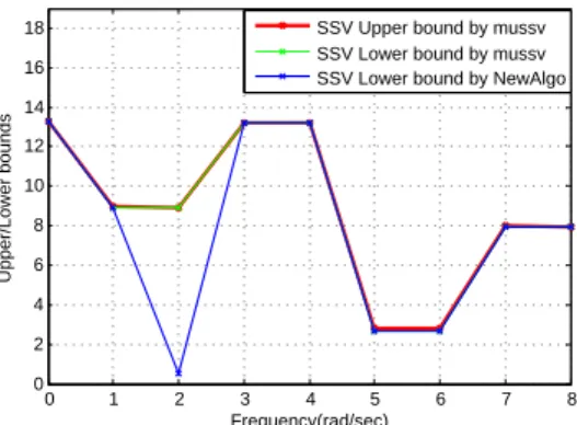
In this case, ∗ = 1.0000 and k℘∗k₂ = 0.0641. The obtained lower bound is as µlower_{N ew} = 15.5995.

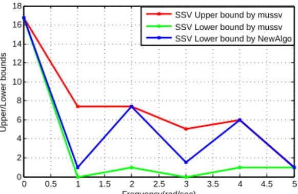
In the following Figure 2, we give the comparison of lower bounds of structured singular values approximated by our New algorithm with the Lower and Upper bounds

A3 =

     

0 0 1 0 0

0 0 0 1 0

1 0 0 0 0

0 1 0 0 0

−1 −1 −1 −1 −1       .

(9)

b ℘=      

0.4354 0 0 0 0

0 0.4354 0 0 0

0 0 0.0337 0.0337 −0.2740

0 0 0.0226 0.0226 −0.1840

      .

Thek℘_bk2 = 0.4354.The computed upper bound isµupper_{P D} = 2.2966. The same lower bound

is obtained, that is, µlower_{P D} = 2.2966. By using algorithm [11], the perturbation structure

℘∗ =      

1.0000 0 0 0 0

0 1.0000 0 0 0

0 0 0.0773 0.0774 −0.6293

0 0 0.0519 0.0520 −0.4227

      .

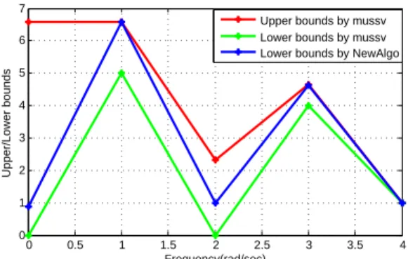
In this case, ∗ = 1.0000 and k℘∗k₂ = 2.2966. The obtained lower bound is as µlower

N ew = 0.4354.

A4 =

     

0 0 1 0 0

0 0 0 1 0

1 0 0 0 0

0 1 0 0 0

−1 −1 −1 −1 −1       .

Θ_B0 ={diag(δ₁I₁, δ₂I₁, ℘₁) :δ₁, δ₂ ∈_R, ℘₁∈_C3,3}.

b ℘=      

0.4354 0 0 0 0

0 0.4354 0 0 0

0 0 0.0337 0.0337 −0.2740

0 0 0.0226 0.0226 −0.1840

(10)

REFERENCES 853

Thek℘_bk₂ = 0.4354.The computed upper bound isµupper_{P D} = 2.2966. The same lower bound is obtained, that is, µlower_{P D} = 2.2966. By using algorithm [11], the perturbation structure

℘∗ = 

    

1.0000 0 0 0 0

0 1.0000 0 0 0

0 0 0.0773 0.0774 −0.6293

0 0 0.0519 0.0520 −0.4227



    

.

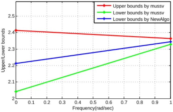
In this case, ∗ = 1.0000 and k℘∗k2 = 2.2966. The obtained lower bound is as µlower_{N ew} =

0.4354.

In the following Figures [5-14], we give the comparison of lower bounds of structured singular values approximated by our New algorithm with the Lower and Upper bounds approximated by MATLAB function mussv for the various matrix valued functions.

6. Conclusion

In this article we have considered the numerical approximation ofµ-values for the matrix

representations of finite symmetric groupsSn over the filed of complex numbers by using

well-known MATLAB function mussv and our algorithm [11]. The experimental results

indicates the different behaviors of lower bounds ofµ-values with once computed by mussv

and our algorithm.

References

[1] Bernhardsson, Bo and Rantzer, Anders and Qiu, Li. Real perturbation values and real quadratic forms in a complex vector space. Linear algebra and its applications, Volume 1: 131-154, 1994.

[2] Braatz, Richard P and Young, Peter M and Doyle, John C and Morari, Manfred.

Computational complexity ofµcalculation. Automatic Control, IEEE Transactions

on, Volume 39: 1000-1002, 1994.

(11)

Appendix 854

[4] Fan, Michael KH and Tits, Andr´e L and Doyle, John C. Robustness in the presence

of mixed parametric uncertainty and unmodeled dynamics. Automatic Control,

IEEE Transactions on, Volume 36: 25-38, 1991.

[5] Hinrichsen, D and Pritchard, AJ. Mathematical systems theory I, vol. 48 of Texts in Applied Mathematics. Springer-Verlag, Berlin Volume 48: 2005.

[6] Karow, Michael and Kokiopoulou, Effrosyni and Kressner, Daniel. On the compu-tation of structured singular values and pseudospectra. Systems & Control Letters Volume 59: 122-129, 2010.

[7] Karow, Michael and Kressner, Daniel and Tisseur, Fran¸coise. Structured eigenvalue

condition numbers. SIAM Journal on Matrix Analysis and Applications Volume 28: 1052-1068, 2006.

[8] Packard, Andrew and Doyle, John. The complex structured singular value. Auto-matica Volume 29: 71-109, 1993.

[9] Packard, Andy and Fan, Michael KH and Doyle, John. A power method for the structured singular value. Decision and Control, 1988., Proceedings of the 27th IEEE Conference on, 2132-2137, 1998.

[10] Qiu, Li and Bernhardsson, Bo and Rantzer, Anders and Davison, EJ and Young, PM and Doyle, JC. A formula for computation of the real stability radius. Automatica, 879-890, 1995.

[11] Rehman, Mutti-Ur and Tabassum, Shabana Numerical Computation of Structured

Singular Values for Companion Matrices. Journal of Applied Mathematics and

Physics volume. 5, number. 5, pages. 1057, year. 2017.

[12] Doyle, John Analysis of feedback systems with structured uncertainties. IEE Pro-ceedings D-Control Theory and Applications volume. 129. number 6. pages 242–250. year 1982. organization IET.

[13] Ferreres, Gilles A practical approach to robustness analysis with aeronautical appli-cations. Springer Science & Business Media year 1999.

[14] Fu, Minyue The real structured singular value is hardly approximable. IEEE Trans-actions on Automatic Control year 1997.

[15] Newlin, Matthew P and Glavaski, Sonja T Advances in the computation of the/spl mu/lower bound. American Control Conference, Proceedings of the 1995 year 995.

(12)

Appendix 855

0 1 2 3 4 5 6 7 8

0.5 1 1.5 2 2.5 3

Frequency(rad/sec)

Upper/Lower bounds

SSV Upper bound by musv SSV Loweer bound by musv SSV Lower bound by NewAlgo

(13)

Appendix 856

0 1 2 3 4 5 6 7 8

0 2 4 6 8 10 12 14 16 18

Frequency(rad/sec)

Upper/Lower bounds

SSV Upper bound by mussv SSV Lower bound by mussv SSV Lower bound by NewAlgo

(14)

Appendix 857

0 1 2 3 4 5

0 0.2 0.4 0.6 0.8 1 1.2 1.4 1.6

Frequency(rad/sec)

Upper/Lower bounds

(15)

Appendix 858

0 0.1 0.2 0.3 0.4 0.5 0.6 0.7 0.8 0.9 1 4

4.5 5 5.5

Frequency(rad/sec)

Upper/Lower bounds

SSV Upper bounds by mussv SSV Lower bounds by mussv SSV Lower bounds by NewAlgo

(16)

Appendix 859

0 0.5 1 1.5 2 2.5 3 3.5 4 4.5 5 0

2 4 6 8 10 12 14 16 18

Frequency(rad/sec)

Upper/Lower bounds

(17)

Appendix 860

0 0.5 1 1.5 2 2.5 3 3.5 4

0 1 2 3 4 5 6 7

Frequency(rad/sec)

Upper/Lower bounds

Upper bounds by mussv Lower bounds by mussv Lower bounds by NewAlgo

(18)

Appendix 861

0 1 2 3 4 5

0 0.5 1 1.5

Frequency(rad/sec)

Upper/Lower bounds

(19)

Appendix 862

0 0.1 0.2 0.3 0.4 0.5 0.6 0.7 0.8 0.9 1 2

2.1 2.2 2.3 2.4 2.5

Frequency(rad/sec)

Upper/Lower bounds

(20)

Appendix 863

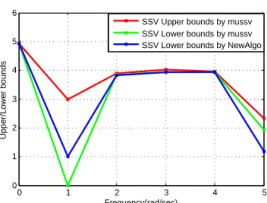
0 1 2 3 4 5

0 1 2 3 4 5 6

Frequency(rad/sec)

Upper/Lower bounds

(21)

Appendix 864

0 0.1 0.2 0.3 0.4 0.5 0.6 0.7 0.8 0.9 1 0

1 2 3 4 5

Frequency(rad/sec)

Upper/Lower bounds

(22)

Appendix 865

0 1 2 3 4 5

2.5 3 3.5 4 4.5 5 5.5 6

Frequency(rad/sec)

Upper/Lower bounds

SSV Upper bound by mussv SSV Lower bounds by mussv SSV Lower bounds by NewAlgo

(23)

Appendix 866

0 0.2 0.4 0.6 0.8 1 1.2 1.4 1.6 1.8 2 4.5

5 5.5 6 6.5 7 7.5 8

Frequency(rad/sec)

Upper/Lower bounds

Upper bounds by mussv Lower bounds by mussv Upper bounds by NewAlgo

(24)

Appendix 867

0 0.5 1 1.5 2 2.5 3 3.5 4

1 1.5 2 2.5

Frequency(rad/sec)

Upper/Lower bounds

(25)

Appendix 868

0 0.2 0.4 0.6 0.8 1 1.2 1.4 1.6 1.8 2 0

0.5 1 1.5 2 2.5

Frequency(rad/sec)

Upper/Lower bounds