Authors are encouraged to submit new papers to INFORMS journals by means of a style file template, which includes the journal title. However, use of a template does not certify that the paper has been accepted for publication in the named jour-nal. INFORMS journal templates are for the exclusive purpose of submitting to an INFORMS journal and should not be used to distribute the papers in print or online or to submit the papers to another publication.
Dynamic Facility Location with Generalized
Modular Capacities
Sanjay Dominik Jena
Centre interuniversitaire de recherche sur les r´eseaux d’entreprise, la logistique et le transport (CIRRELT) and D´epartement d’informatique et de recherche op´erationnelle, Universit´e de Montr´eal, [email protected],
Jean-Fran¸cois Cordeau
Centre interuniversitaire de recherche sur les r´eseaux d’entreprise, la logistique et le transport (CIRRELT) and Canada Research Chair in Logistics and Transportation, HEC Montr´eal, [email protected],
Bernard Gendron
Centre interuniversitaire de recherche sur les r´eseaux d’entreprise, la logistique et le transport (CIRRELT) and D´epartement d’informatique et de recherche op´erationnelle, Universit´e de Montr´eal, [email protected]
Location decisions are frequently subject to dynamic aspects such as changes in customer demand. Often,
flexibility regarding the geographic location of facilities, as well as their capacities, is the only solution to such
issues. Even when demand can be forecast, finding the optimal schedule for the deployment and dynamic
adjustment of capacities remains a challenge, especially when the cost structure for these adjustments is
complex. In this paper, we introduce a unifying model that generalizes existing formulations for several
dynamic facility location problems and provides stronger linear programming relaxations than the specialized
formulations. In addition, the model can address facility location problems where the costs for capacity
changes are defined for all pairs of capacity levels. To the best of our knowledge, this problem has not been
addressed in the literature. We apply our model to special cases of the problem with capacity expansion
and reduction or temporary facility closing and reopening. We prove dominance relationships between our
formulation and existing models for the special cases. Computational experiments on a large set of randomly
generated instances with up to 100 facility locations and 1000 customers show that our model can obtain
optimal solutions in shorter computing times than the existing specialized formulations.
Key words: Mixed-Integer Programming, Facility Location, Modular Capacities
1.
Introduction
Dynamic facility location consists in decidingwhere and when to provide capacity to satisfy
cus-tomer demand at the lowest cost. This demand is rarely stable, but rather increases, decreases or
oscillates over time. Therefore, facility capacities often have to be adjusted dynamically. Many
vari-ants of dynamic facility location problems have been studied, suggesting different ways to adjust
capacities throughout a given planning horizon. The most common features include capacity
expan-sion and reduction (Luss 1982, Jacobsen 1990, Peeters and Antunes 2001, Troncoso and Garrido
2005, Dias et al. 2007), temporary facility closing (Chardaire et al. 1996, Canel et al. 2001, Dias
et al. 2006), as well as the relocation of capacities (Melo et al. 2006). Mathematical models that
include such features have been applied in both the private and the public sectors to determine
locations and capacities for production facilities, schools, hospitals, libraries and many more.
Facility location decisions aim to strike a balance between the fixed costs to supply capacity and
the allocation costs to serve the demand. The latter often correspond to transportation costs to
deliver products or provide services to customers. The ratio between these two types of costs has
a strong impact on the solution and the difficulty of solving the problem (see, e.g., Shulman 1991,
Melkote and Daskin 2001). In dynamic facility location problems, a detailed representation of the
transportation costs not only affects the facility locations, but also their capacity throughout the
planning horizon as capacity tends to follow the demand along time.
Regarding the fixed costs to provide the capacity, many studies acknowledge the existence of
economies of scale (Correia and Captivo 2003, Correia et al. 2010). While previous works
consid-ered economies of scale mainly for the construction and production costs, the costs for adjusting
the capacities of the facilities have commonly been modeled in less detail. However, the latter
is necessary to ensure a fair representation of the cost structure found in practice. The costs to
adjust capacities often do not only depend on the size of the adjustment, but also on the current
capacity level. This is true in a large class of applications, especially in transportation, logistics and
telecommunications, where additional capacity gets cheaper (or more expensive) when approaching
In this work, we introduce a very general dynamic facility location problem, referred to as the
Dynamic Facility Location Problem with Generalized Modular Capacities (DFLPG). The problem
allows modular capacity changes subject to a detailed cost structure and is modeled as a
mixed-integer programming (MIP) formulation. Due to its generality, this model unifies several existing
problems found in the literature. The cost structure used in the model is based on a matrix
describing the costs for capacity changes between all pairs of capacity levels. We are not aware of
any other work dealing with facility location with a similar level of detail in the cost structure.
Our study is motivated by an industrial project with a Canadian logging company that must
locate camps to host workers involved in wood harvest activities while optimizing the overall
logistics and transportation costs (Jena et al. 2012). In this problem, the total capacity of a camp is
represented by its number of hosting units, while additional units provide supporting infrastructure.
As the relation between the number of different units is non-linear, the costs for capacity changes
are described in a transition matrix.
The contribution of this work is threefold. First, we introduce a general dynamic facility location
model that comprises a large set of existing formulations. Second, we analyze the linear
program-ming (LP) relaxation bound obtained by our model, showing that it is at least as strong as the LP
relaxation bound of existing specialized formulations. Third, we perform a computational study on
a large set of randomly generated instances, showing that our model, when solved with a
state-of-the-art MIP solver, can obtain optimal solutions in shorter computation times than the specialized
formulations.
The paper is organized as follows. In Section 2, we present a survey of the relevant literature.
Section 3 introduces a linear MIP formulation for the DFLPG and shows how this model can be
used to represent two important special cases. To compare the resulting models with alternative
formulations, Section 4 derives specialized formulations for the two special cases, based on existing
models from the literature. We identify a weak point in one of the existing formulations and suggest
between all formulations, showing that our model is at least as strong as each of the specialized
formulations. The presented models are then compared by means of computational experiments in
Section 5. Finally, conclusions follow in Section 6.
2.
Literature Review
Most dynamic facility location problems can be seen as multi-periodic extensions of classical
loca-tion problems, such as the Capacitated Facility Localoca-tion Problem (CFLP). However, dynamic
facility location problems commonly involve further extensions. As pointed out by Arabani and
Farahani (2011), the notion of what dynamic means may differ when dealing with different areas
of facility location. Its definition thus strongly depends on the application context. For example,
school capacities may be increased or decreased to meet demographic trends (e.g., Peeters and
Antunes 2001), terminals in telecommunications networks may be installed and removed along time
to adapt to changes in data traffic and costs (e.g., Chardaire et al. 1996) and hospitals may relocate
ambulances to cope with unpredictable demand (e.g., Brotcorne et al. 2003). Owen and Daskin
(1998) review works that treat either dynamic or stochastic facility location problems. A chapter
in the textbook of Farahani and Hekmatfar (2009) deals with dynamic aspects of facility location
problems. Several classification criteria are proposed. A book chapter by Jacobsen (1990)
dedi-cated to multi-period capacitated location models thoroughly discusses models that allow capacity
expansion. Luss (1982) focuses on capacity expansion and reviews the literature and applications
in the context of problems with a single facility, two facilities and multiple facilities. Although not
explicitly focusing on dynamic aspects, many other works introduced classifications for location
problems which often also apply to features that can be found in dynamic location problems. These
include, among many others, the works of Hamacher and Nickel (1998), Owen and Daskin (1998),
Klose and Drexl (2005), Daskin (2008) and Melo et al. (2009).
The choice of the facility type or size has also been considered in several works. In particular,
Shulman (1991), Correia and Captivo (2003) and Troncoso and Garrido (2005) consider such choice,
to the forestry sector, where facilities of different sizes may also be expanded. Dias et al. (2007) focus
on modular capacity expansion and reduction. Wu et al. (2006) present a facility location problem
where the facility setup costs depend on the number of facilities placed at a site. To represent
economies of scale, all of the cited works use binary variables to distinguish different facility sizes.
Capacity level changes consider only the amount of capacity added or removed. However, the
previous capacity level is not taken into consideration. Some authors such as Harkness (2003) also
recognize the importance of inverse economies of scale, where the unit price increases as the facility
gets larger.
To dynamically adjust capacity to demand changes, the best choice depends on the demand
fore-cast and the costs involved in capacity changes. For example, if capacity is leased, it may be possible
to terminate a leasing contract at any time. In other situations, it may be beneficial to temporarily
close a facility to avoid high maintenance costs. This may be appropriate when demand
temporar-ily decreases, but is likely to return to its previous level afterwards. The closing and reopening of
facilities may be partial or complete. Previous studies focused mostly on temporarily closing entire
facilities. Among the suggested models, certain are limited to a single closing and reopening of each
facility, whereas others allow repeated closing and reopening throughout the planning horizon. The
uncapacitated facility location problem presented by Van Roy and Erlenkotter (1982), as well as
the supply chain model of Hinojosa et al. (2008), allow one-time opening or closing of facilities: new
facilities can be opened once and existing facilities can be closed once. Chardaire et al. (1996) and
Canel et al. (2001) propose formulations for opening and closing facilities more than once. Both
works use binary variables to represent the state of the facility. The objective function contains a
bilinear term to represent a state change from open to closed or vice-versa. A linear formulation
for a simplified version of this problem, treating only a single capacity level, has been proposed by
Dias et al. (2006). Binary variables with two time indices indicate the period throughout which a
facility is open. The cited works interpret facility closing either as temporary (i.e., the facility still
costs for temporarily closed facilities are low and can therefore be ignored in the model. Most of
the existing formulations therefore do not explicitly distinguish temporary and permanent facility
closing.
When the customer demand permanently changes in a certain region and is not likely to return
to its previous level, one may want to expand or reduce the facility capacities to permanently adjust
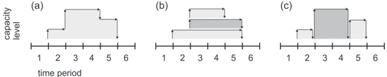
to these new conditions. Luss (1982) observes that models for capacity expansion can be classified
into two categories: capacity expansion at a single facility and capacity expansion via a finite set of
projects, each holding a certain capacity. The first category includes models that allow one facility
at a location and increases or decreases of the available capacity along time. The second category
consists of models where multiple facilities are allowed in the same location, each specified by a
time interval (a capacity block) of production availability. Figure 1 illustrates both classes. The
first class is shown in (a), where capacities at the same facility are either increased or decreased.
The second class may be illustrated by (b) and (c), representing two extreme configurations of the
capacity blocks. Any configuration between these two is also feasible for the second class.
(a)
capacity level
time period
1 2 3 4 5 6
1 2 3 4 5 6 1 2 3 4 5 6
(c) (b)
Figure 1 Capacity expansion/reduction by use of a single facility (a), horizontal capacity blocks (b) and vertical
capacity blocks (c).
Models in the first category include those of Melo et al. (2006) and Behmardi and Lee (2008).
Both works model capacity expansion and reduction by relocating capacity from or to a dummy
location. The authors of the former work model capacities as a continuous flow, but demonstrate
how to link the flow to binary variables to restrict capacity changes to modular sizes. Models in the
second category do not allow the capacity modification of a facility once it is constructed. However,
equivalent to the adjustment of the total capacity sum along time. Examples for this class include
the works of Shulman (1991), Troncoso and Garrido (2005) and Dias et al. (2007). More restricted
types of capacity expansion or reduction have also been presented. In the work of Peeters and
Antunes (2001), either a facility expands or decreases its capacity throughout the entire planning
horizon. Capacity expansion and reduction at the same location is thus not allowed.
3.
Mathematical Formulation
In this section, we give a more formal description of the DFLPG and introduce a MIP model for
the problem. We also explain how the different cases described in Section 2 can be modeled as a
DFLPG.
3.1. DFLPG Formulation
We denote byJ the set of potential facility locations and byL={0,1,2, . . . , q} the set of possible
capacity levels for each facility. We also denote by I the set of customer demand points and by
T={1,2, . . . ,|T|}the set of time periods in the planning horizon. We assume throughout that the
beginning of periodt+ 1 corresponds to the end of period t.
The demand of customeriin periodtis denoted bydit. The cost to serve one unit from facilityj
operating at capacity level`to customeriduring periodtis denoted bygij`t. This term is typically
a cost function for handling and transportation costs, based on the distance between customer i
and facility j. The capacity of a facility of size` at locationj is given byuj` (with uj0= 0). The
cost matrixfj`1`2tdescribes the combined cost to change the capacity level of a facility at locationj
from`1to`2 at the beginning of periodtand to operate the facility at capacity level`2 throughout
time periodt. Furthermore, we let`j be the capacity level of an existing facility at locationj. The
constant`j is 0 if location j does not possess an existing facility at the beginning of the planning
horizon.
To formulate the problem, we use binary variables yj`1`2t equal to 1 if and only if the facility
at location j changes its capacity level from `1 to`2 at the beginning of period t. The allocation
a facility of size ` located at j. Based on these definitions, we define the following MIP model,
referred to as theGeneralized Modular Capacities (GMC) formulation:
(GMC) minX
j∈J X
`1∈L X
`2∈L X
t∈T
fj`1`2tyj`1`2t+ X
i∈I X
j∈J X
`∈L X
t∈T
gij`tditxij`t (1)
s.t. X j∈J
X
`∈L
xij`t= 1 ∀i∈I, ∀t∈T (2)
X
i∈I
ditxij`t≤ X
`1∈L
uj`yj`1`t ∀j∈J, ∀`∈L, ∀t∈T (3)
X
`1∈L
yj`1`(t−1)= X
`2∈L
yj``2t ∀j∈J, ∀`∈L, ∀t∈T\ {1} (4)
X
`2∈L yj`j`
21= 1 ∀j∈J (5)
xij`t≥0 ∀i∈I, ∀j∈J, ∀`∈L, ∀t∈T (6)
yj`1`2t∈ {0,1} ∀j∈J, ∀`1∈L, ∀`2∈L, ∀t∈T. (7)
The objective function (1) minimizes the total cost for changing the capacity levels and allocating
the demand. Constraints (2) are the demand constraints for the customers. Constraints (3) are
the capacity constraints at the facilities. Constraints (4) link the capacity change variables in
consecutive time periods. Finally, constraints (5) specify that exactly one capacity level must be
chosen at the beginning of the planning horizon. Note that the flow constraints (4) further guarantee
that, at each time period, exactly one capacity change variable is selected.
Valid Inequalities. To facilitate the solution of the GMC, we may additionally use two types of
valid inequalities. TheStrong Inequalities (SI)used in facility location and network design problems
(see, for instance, Gendron and Crainic 1994) are known to provide a tight upper bound for the
demand assignment variables. These inequalities can be adapted to our model as follows:
xij`t≤ X
`1∈L
yj`1`t ∀i∈I, ∀j∈J, ∀`∈L, ∀t∈T. (8)
The SIs may be added to the model eithera priori or in a branch-and-cut manner only when they
as theAggregated Demand Constraints (ADC). Although they are redundant for the LP relaxation,
adding them to the model enables MIP solvers to generate cover cuts that further strengthen the
formulation:
X
j∈J X
`1∈L X
`2∈L
uj`2yj`1`2t≥ X
i∈I
dit ∀t∈T. (9)
3.2. DFLPG Based Models for the Special Cases
We now explain how two important special cases can be modeled with the GMC formulation: first,
Facility closing and reopening and, second,Capacity expansion and reduction.
The first problem considered here allows the construction of at most one facility per location.
The size of the facility is chosen from a discrete set of capacity levels. Existing facilities may be
closed and reopened multiple times. Note that, in this problem, facility closing does not refer to
permanent closing, but only to the temporary closing of a facility. We therefore distinguish costs
for the construction of a facility, for temporarily closing an open facility, for reopening a closed
facility and for maintenance of open facilities. As most of the previous literature, we do not consider
maintenance costs for temporarily closed facilities. We denote this problem as theDynamic Modular
Capacitated Facility Location Problem with Closing and Reopening (DMCFLP CR).
In the second problem considered, capacities can be adjusted by the use of a single facility at
each location. At each facility, the capacity can be expanded or reduced from one capacity level to
another. We assume that an expansion of ` capacity levels has always the same costs, regardless
of the previous capacity level. We assume the same for the reduction of capacities. We denote this
problem as theDynamic Modular Capacitated Facility Location Problem with Capacity Expansion
and Reduction (DMCFLP ER).
In addition to the input data already defined for the DFLPG, we define the following fixed costs
to characterize these two special cases:
• cc
j` and c o
j` are the costs to temporarily close and reopen a facility of size ` at location j,
• fc j` and f
o
j` are the costs to reduce and to expand the capacity of a facility at location j by `
capacity levels, respectively;
• Fo
j` is the cost to maintain an open facility of size`at locationj throughout one time period.
For the sake of simplicity and without loss of generality, we assume that all these costs do not
change during the planning horizon.
In the GMC, capacity level changes are represented by the yj`1`2t variables. These transitions
from one capacity level to another can be represented in a graph, where each node represents a
capacity level and each arc a capacity level transition. To model the special cases, we choose a
certain subset of arcs, as well as their corresponding objective function coefficients fj`1`2t. Note
that, while the costs for the GMC can be based on a cost matrix, the costs for the special cases
are based on a cost vector. The cost coefficients fj`1`2t correspond to combinations of different
operations, for example the cost to expand capacity plus the maintenance costs for the new capacity
level.
For the problem variant involving facility closing and reopening, we create an artificial capacity
level`for each capacity level `∈L\{0}. Capacity level `represents the state in which a facility of
size`is temporarily closed. At each time period t∈T and location j∈J, we may find different arc
typesyj`1`2t to model capacity level changes (note that the cost for an arc is usually composed by
the cost to perform the capacity transition, as well as the maintenance costs for the new capacity
level):
1. Facility construction and capacity expansion. The expansion of the capacity is represented
by an arc from capacity level`1 to any other capacity level`2> `1. If the arc represents a facility
construction, then `1 is 0. The capacity is thus expanded by `2−`1 capacity levels. The cost for
this arc is set to fj`1`2t=f o
j(`2−`1)+F o j`2.
2. Capacity reduction. The reduction of the capacity is represented by an arc from capacity level
`1 to any other capacity level `2< `1. The capacity is thus reduced by`1−`2 capacity levels. The
3. Maintaining the current capacity level. A facility may neither expand nor reduce the current
capacity level. The cost of this arc is thus only composed of the maintenance cost, i.e., fj`1`1t=
Fo
j`1 if the capacity level represents an open facility, fj`1`1t= 0 if the capacity level represents a
temporarily closed facility andfj00t= 0 if no facility exists.
4. Temporary closing. An open facility of size `1 can be temporarily closed, i.e., it changes to
capacity level`1. The total cost isfj`1`1t=c c j`1.
5. Reopening a closed facility. A temporarily closed facility of size `1 can be reopened, i.e., it
changes its capacity level from `1 to`1. The total cost for this arc isfj`1`1t=c o j`1+F
o j`1.
The DMCFLP CR is represented by arcs of type 1 (for construction only), 3, 4 and 5. We denote
the resulting model as theCR-GMC formulation. The DMCFLP ER is represented by arcs of type
1, 2 and 3. The resulting model is denoted as the ER-GMC formulation.
4.
Comparisons with Specialized Formulations
We now present alternative formulations for the two special cases discussed in Section 3.2. These
formulations are adaptations of existing models proposed in the literature. For each problem, we
present formulations based on two different modeling approaches as presented in Section 2: location
variables with one time index and location variables with two time indices.
4.1. Facility Closing and Reopening
We consider models for the problem with facility closing and reopening, the DMCFLP CR.
4.1.1. Single Time Index Flow Formulation
This model can be seen as an extension of existing dynamic facility location problems (Shulman
1991). Flow conservation constraints such as those used in the relocation model of Wesolowsky
and Truscott (1975) are adapted to model facility closing and reopening. The model is based on
the following variables. The demand allocation from facilities to customers is given byxij`t. Binary
variablesj`t is 1 if a facility of size`is constructed at the beginning of periodtat locationj, while
binary flow variableyj`t indicates whether a facility of size`is available at location j during time
period t. Finally, binary variables vo
j`t and v c
location j of size `is reopened at the beginning of period tand if an open facility at location j of
size`is temporarily closed at the beginning of period t, respectively. The input data is as defined
in Section 3.2. Note that certain equations may include terms which are not defined for a certain
variable index, e.g., index (t−1) is not defined fort= 1. Undefined terms are assumed to take the
value 0. The single time index flow formulation (CR-1I) is given by:
(CR-1I) minX
j∈J X
`∈L X
t∈T
fo
j`sj`t+Fj`oyj`t+coj`v o j`t+c
c j`v c j`t +X
i∈I X
j∈J X
`∈L X
t∈T
gij`tditxij`t (10)
s.t. X j∈J
X
`∈L
xij`t= 1 ∀i∈I, ∀t∈T (11)
X
i∈I
ditxij`t≤uj`yj`t ∀j∈J, ∀`∈L, ∀t∈T (12)
yj`t=yj`(t−1)+sj`t+voj`t−v c
j`t ∀j∈J, ∀`∈L, ∀t∈T (13) t
X
t0=1 voj`t0≤
t X
t0=1
vj`tc 0 ∀j∈J, ∀`∈L, ∀t∈T (14)
X
`∈L X
t∈T
sj`t≤1 ∀j∈J (15)
xij`t≥0 ∀i∈I, ∀j∈J, ∀`∈L, ∀t∈T (16)
sj`t, voj`t, v c
j`t, yj`t∈ {0,1} ∀j∈J, ∀`∈L, ∀t∈T. (17)
The objective function (10) minimizes the total costs composed by facility construction,
main-tenance of open facilities and facility reopening and closing, as well as the costs to satisfy the
customer demand. Constraints (11) are the demand constraints. Constraints (12) are the
capac-ity constraints. The flow constraints (13) manage the state of a facilcapac-ity of a certain size, either
open or closed. Constraints (14) ensure that a facility has to be temporarily closed before it can
be reopened. Finally, constraints (15) state that at most one facility can be constructed at each
location.
The Strong Inequalities (8) can be adapted by replacing the right-hand side by yj`t, while
the Aggregated Demand Constraints (9) can be used by replacing the left-hand side by
P j∈J
P
4.1.2. Double Time Index Block Formulations
Dias et al. (2006) presented a linear MIP model that allows the repeated closing and reopening
of facilities. The model uses binary decision variables with two time indices, one for the opening
and one for the closing of a facility. We extend this model by adding the choice of different facility
capacity levels (note that we remove the constraints that require a minimum availability of open
facilities). We also use a different notation to be consistent with our previously introduced notations.
Binary variablesj`t1t2 is 1 if a facility of size `is constructed at locationj at the beginning of time
periodt1and stays open until the end of periodt2. Binary variableyj`t1t2 is 1 if an existing facility
of size `, located atj, is reopened at the beginning of time period t1 and stays open until the end
of period t2. We let ˆfj`tC1t2 denote the aggregated cost to construct a facility of size ` at location
j at time period t1, its maintenance costs from the beginning of period t1 to the end of period t2,
and the costs to temporarily close it at the end of period t2. We also let ˆfj`tR1t2 denote the same
type of cost for reopening an existing facility of size `instead of its construction. These constants
are computed as follows:
ˆ
fC j`t1t2=f
o j`+c
c
j`+ (t2−t1+ 1)Fj`o and fˆ R j`t1t2=c
o j`+c
c
j`+ (t2−t1+ 1)Fj`o.
Since the binary variables with two time indices describe capacity blocks through time, we refer to
this formulation as thedouble time index block formulation (CR-2I):
(CR-2I) minX
j∈J X
`∈L X
t1∈T |T|
X
t2=t1
ˆ
fC
j`t1t2sj`t1t2+ ˆf R
j`t1t2yj`t1t2
+X
i∈I X
j∈J X
`∈L X
t∈T
gij`tditxij`t (18)
s.t. X j∈J
X
`∈L
xij`t= 1 ∀i∈I, ∀t∈T (19)
|T|
X
t2=t
yj`tt2≤ t−1 X
t1=1 t−1 X
t2=t1
sj`t1t2 ∀j∈J, ∀`∈L, ∀t∈T (20)
X
`∈L X
t1∈T
|T|
X
t2=t1
sj`t1t2 ≤1 ∀j∈J (21)
X
`∈L t X
t1=1 |T|
X
t2=t
X
i∈I
ditxij`t≤ t X
t1=1 |T|
X
t2=t
uj`(sj`t1t2+yj`t1t2) ∀j∈J, ∀`∈L, ∀t∈T (23)
xij`t≥0 ∀i∈I, ∀j∈J, ∀`∈L, ∀t∈T (24)
sj`t1t2, yj`t1t2∈ {0,1} ∀j∈J, ∀`∈L, ∀t1∈T, ∀t2∈T. (25)
Constraints (19) are the demand constraints. Constraints (20) guarantee that a facility can only
be reopened if it has been constructed and temporarily closed in an earlier period. Inequalities
(21) impose that a facility can be constructed only once throughout the entire planning horizon.
Constraints (22) guarantee that the intervals of open facilities (i.e., the capacity blocks) at the
same location do not intersect. In other words, a facility can only be reopened if it is currently
closed. In addition, these constraints also require that only one facility size ` is selected at each
location. Constraints (23) are the facility capacity constraints.
The Strong Inequalities (8) can be adapted by replacing the right-hand side by
Pt t1=1
P|T|
t2=t(sj`t1t2+yj`t1t2). The Aggregated Demand Constraints (9) can be used by replacing
the left-hand side by P j∈J
P `∈L
Pt t1=1
P|T|
t2=tuj`(sj`t1t2+yj`t1t2).
Strengthening the CR-2I formulation. Constraints (20) specify that, at each time periodt, the
capacity that is reopened at this period cannot be greater than the capacity that has been previously
constructed. Consider the following LP relaxation solution scenario, where demands exist for three
time periodst1,t2andt3. A facility construction variable is selected with solution value 0.5, opening
at the beginning of t1 and closing at the end of t1 (i.e., sj`t1t1= 0.5). Facility reopening variables
are then selected twice, each time with the same solution value 0.5. The first reopening spans the
time interval from the beginning of t2 until the end of t3 (i.e., yj`t2t3 = 0.5), whereas the second
reopening spans the time interval from the beginning of t3 until the end of t3 (i.e., yj`t3t3 = 0.5).
Separately, each of the last two reopenings is feasible in constraints (20). However, in total the
solution reopens more capacity than has been made available through construction. To avoid such
behaviour in the LP relaxation solution, we may replace constraints (20) with the tighter set of
constraints:
t X
t1=1 |T|
X
t2=t
yj`t1t2 ≤ t X
t1=1 t X
t2=t1
We denote the formulation given by (18), (19) and (21) - (26) as the CR-2I+ formulation.
4.1.3. Dominance Relationships
For any integer linear programming model P, let P be the corresponding LP relaxation. For any
modelP, we denote byv(P) its optimal value. For the three models presented for the DMCFLP CR,
the following relationships hold:
Theorem 1. v(CR-GMC) =v(CR-1I)≥v(CR-2I).
Proof. See Appendices A.1.1 (Theorem 4) and A.1.2 (Theorem 5).
If constraints (20) in the CR-2I formulation are replaced by the strengthening constraints (26),
all three formulations are equally strong:
Theorem 2. v(CR-GMC) =v(CR-1I) =v(CR-2I+).
Proof. See Appendix A.1.3 (Theorems 4 and 7).
4.2. Capacity Expansion and Reduction
We consider models for the facility location problem with capacity expansion and reduction, the
DMCFLP ER.
4.2.1. Single Time Index Flow Formulation
We modify the CR-1I as follows. Binary variables sj`t now represent the total capacity expansion.
A variablesj`t is 1 if the capacity of the facility located atj is expanded by`capacity levels at the
beginning of period t. Binary variablewj`t is 1 if the capacity of a facility located atj is reduced
by ` capacity levels at the beginning of period t. We refer to this formulation as the single time
index flow formulation (ER-1I):
(ER-1I) minX j∈J
X
`∈L X
t∈T
fo
j`sj`t+fj`cwj`t+Fj`oyj`t
+X
i∈I X
j∈J X
`∈L X
t∈T
gij`tditxij`t (27)
s.t. (11),(12)
X
`∈L
`yj`t= X
`∈L
`yj`(t−1)+`sj`t−`wj`t
X
`∈L
yj`t≤1 ∀j∈J, ∀t∈T (29)
X
`∈L
sj`t≤1 ∀j∈J, ∀t∈T (30)
X
`∈L
wj`t≤1 ∀j∈J, ∀t∈T (31)
xij`t≥0 ∀i∈I, ∀j∈J, ∀`∈L, ∀t∈T (32)
sj`t, wj`t, yj`t∈ {0,1} ∀j∈J, ∀`∈L, ∀t∈T. (33)
Now, the flow conservation constraints (28) manage the size of the facilities throughout the planning
periods. Constraints (29) - (31), referred to as thelimiting constraints, guarantee that the solution
selects at most one capacity level for each type of variable y,sand w, respectively. If the costs for
facility maintenance, capacity expansion and capacity reduction include economies of scale, these
constraints are redundant, because the optimal solution will always choose a single capacity level:
the one with the lowest cost in relation to its capacity.
The model may be seen as an adaptation of the relocation model of Wesolowsky and Truscott
(1975), where capacity is expanded or reduced instead of relocated. It is also similar to the model
presented by Jacobsen (1990) and to simplifications of the models presented by Melo et al. (2006)
and Behmardi and Lee (2008).
4.2.2. Double Time Index Block Formulations
Dias et al. (2007) allow multiple capacity blocks of different sizes at the same location. For each
block, binary variables define the exact time interval during which the block is active. This
accumu-lation of capacity blocks allows flexible capacity expansion and reduction as previously discussed
and exemplified in Figure 1 (b) and (c). We extend this formulation to model the DMCFLP ER.
Binary variables yj`t0 1t2 indicate whether a capacity block of size`is available at location j from
the beginning of time period t1 until the end of time period t2. Each capacity block may thus
represent economies of scale in function of its own size. However, in contrast to the ER-1I, the
economies of scale on the entire capacity involved at each location, we introduce additional binary
variables yj`t, which are 1 if the total capacity summed over all capacity blocks at location j
available at time period t equals `. In the same manner, we introduce variables sj`t and wj`t to
represent the total capacity that is added at a location (i.e., the construction of capacity blocks) or
removed at a location (i.e., the closing of capacity blocks), respectively. Finally, as in the previous
models, xij`t is the fraction of customer i’s demand that is served by a facility of size`at location
j. The double time index block formulation (ER-2I)is given by:
(ER-2I) minX j∈J
X
`∈L X
t∈T
fj`osj`t+fj`cwj`t+Fj`oyj`t
+X
i∈I X
j∈J X
`∈L X
t∈T
gij`tditxij`t (34)
s.t. (11),(12),(29),(30),(31)
X
`∈L
`sj`t= X
`∈L
|T|
X
t2=t
`y0j`tt2 ∀j∈J, ∀t∈T (35)
X
`∈L
`wj`t= X
`∈L t−1 X
t1=1
`yj`t0 1(t−1) ∀j∈J, ∀t∈T (36)
X
`∈L
`yj`t= X
`∈L t X
t1=1 |T|
X
t2=t
`yj`t0 1t2 ∀j∈J, ∀t∈T (37)
xij`t≥0 ∀i∈I, ∀j∈J, ∀`∈L, ∀t∈T (38)
yj`t0 1t2, sj`t, wj`t, yj`t∈ {0,1} ∀j∈J, ∀`∈L, ∀t1∈T, ∀t2∈T. (39)
We adapt the demand and capacity constraints (11) and (12), respectively, from the previous
models. Constraints (35), (36) and (37) are the linking constraints that set the binary variables
to benefit from economies of scale in function of the total capacity involved in each operation and
location. As for the ER-1I formulation, we also add the limiting constraints (29) - (31) as introduced
in Section 4.2.1. The limiting constraints are necessary to ensure that feasible solutions use only
one active variable of each type y, s and w for each location and time period. These constraints
have also proved to facilitate the solution process. We may also add the Strong Inequalities and
4.2.3. Dominance Relationships
For the DMCFLP ER, the ER-GMC formulation is stronger (strictly stronger for some instances)
than the other two formulations:
Theorem 3. v(ER-GMC)≥v(ER-1I) =v(ER-2I).
Proof. See Appendices A.2.2 (Theorem 9) and A.2.1 (Theorem 10).
5.
Computational Experiments
In this section, computational results are reported to illustrate the strength of the different
for-mulations and their performance when using a state-of-the-art MIP solver to find optimal integer
solutions. Computational experiments were performed for the two problem variants, DMCFLP CR
and DMCFLP ER.
A large set of instances has been generated, varying a set of key parameters that were
found to affect the difficulty of the problem. Instances have been generated with the following
dimensions (|J|/|I|): (10/20), (10/50), (50/50), (50/100), (50/250), (100/250), (100/500) and
(100/1000). The highest capacity level at any facility, denoted by q, has been selected such that
q∈ {3,5,10}. Three different networks have been randomly generated on squares of the following
sizes: 300km, 380kmand 450km. We consider two different demand scenarios. In both scenarios,
the demand for each of the customers is randomly generated and randomly distributed over time.
The two scenarios differ in their total demand summed over all customers in each time period. In
the first scenario (regular), the total demand is similar in each time period. The second scenario
(irregular) assumes that the total demand follows strong variations along time and therefore varies
at each time period. Facility construction and operational costs follow concave cost functions, i.e.,
they involve economies of scale. All instances have also been generated with a second cost
sce-nario in which the transportation costs are five times higher. Instances have been generated with
|T|= 12, which may be interpreted as a planning horizon of one year divided into 12 months. This
instance set contains a total of 288 instances. Note that we assume that the problem instances do
parameters used to generate the instances. Furthermore, we refer to Appendix C for details on the
model sizes.
All mathematical models have been implemented in C/C++ using the IBM CPLEX 12.6.0
Callable Library. The code has been compiled and executed on openSUSE 11.3. Each problem
instance has been run on a single Intel Xeon X5650 processor (2.67GHz), limited to 24GB of RAM.
5.1. Linear Relaxation Solution and Integrality Gaps
The different formulations for the two problem variants are now compared by means of their LP
relaxation bounds as well as the time necessary to solve the LP relaxations. All SIs have been added
a priori. The Aggregated Demand Constraints have not been added to these models, since they do
not have any impact on the strength of the LP relaxation. For all instances, the LP relaxation has
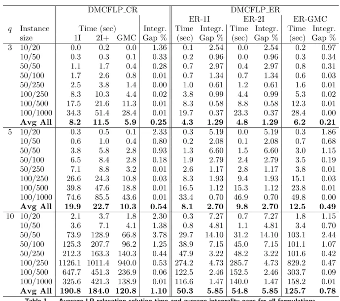
been solved to optimality. Table 1 shows the average times to solve the LP relaxation as well as
the average integrality gaps, for each problem dimension and each number of maximum capacity
levelsq. The optimal integer solutions used to compute the integrality gaps have been obtained by
running CPLEX for up to 24hs.
As previously shown, the CR-1I, the CR-2I+ and the CR-GMC formulations provide the same
LP relaxation bound and thus the same integrality gap. However, the CR-GMC formulation solves
the relaxation in slightly shorter computing times than the CR-1I and CR-2I+ formulations. For
the DMCFLP ER, the ER-1I and ER-2I formulations provide the same integrality gaps. Even
though the computing times for the ER-GMC formulation are higher than for the previous two
formulations, the ER-GMC formulation provides a significantly smaller integrality gap.
5.2. CPLEX Optimization
Generic MIP solvers such as CPLEX incorporate several heuristics to find good quality solutions
early in the search tree and to improve the final solution quality. However, the use of such heuristics
often leads to an unforeseeable behavior and does not allow for a proper comparison of different
formulations for the same problem. We therefore compare the performance of the different
DMCFLP CR DMCFLP ER
ER-1I ER-2I ER-GMC
q Instance Time (sec) Integr. Time Integr. Time Integr. Time Integr.
size 1I 2I+ GMC Gap % (sec) Gap % (sec) Gap % (sec) Gap %
3 10/20 0.0 0.2 0.0 1.36 0.1 2.54 0.0 2.54 0.2 0.97
10/50 0.3 0.3 0.1 0.33 0.2 0.96 0.0 0.96 0.3 0.34
50/50 1.1 1.7 0.4 0.28 0.7 2.97 0.4 2.97 0.8 0.31
50/100 1.7 2.6 0.8 0.01 0.7 1.34 0.7 1.34 0.6 0.03
50/250 2.5 3.8 1.4 0.00 1.0 0.61 1.2 0.61 1.6 0.01
100/250 8.3 10.3 4.4 0.02 3.8 0.99 4.4 0.99 5.3 0.02
100/500 17.5 21.6 11.3 0.01 8.3 0.58 8.8 0.58 12.3 0.01
100/1000 34.3 51.4 28.4 0.01 19.7 0.37 23.3 0.37 28.4 0.00
Avg All 8.2 11.5 5.9 0.25 4.3 1.29 4.8 1.29 6.2 0.21
5 10/20 0.3 0.5 0.1 2.33 0.3 5.19 0.0 5.19 0.3 1.86
10/50 0.6 1.0 0.4 0.80 0.2 2.08 0.1 2.08 0.7 0.68
50/50 3.8 5.8 2.8 0.93 1.3 6.60 1.5 6.60 3.0 1.15
50/100 6.5 8.4 2.8 0.18 1.9 2.79 2.4 2.79 3.5 0.19
50/250 7.1 8.8 3.2 0.01 2.6 1.17 2.8 1.17 3.8 0.01
100/250 26.6 24.3 10.8 0.03 8.3 1.93 9.4 1.93 15.1 0.03
100/500 39.8 47.6 18.8 0.01 16.5 1.12 15.3 1.12 23.8 0.01
100/1000 74.6 85.5 43.6 0.01 33.4 0.70 46.9 0.70 49.8 0.00
Avg All 19.9 22.7 10.3 0.54 8.1 2.70 9.8 2.70 12.5 0.49
10 10/20 2.1 3.7 1.8 2.30 0.3 7.27 0.7 7.27 1.8 1.15
10/50 3.6 7.1 4.1 1.38 0.8 4.81 1.1 4.81 3.4 0.70
50/50 73.9 128.9 66.8 3.78 29.7 14.10 31.2 14.10 103.1 2.44
50/100 125.3 207.7 96.2 1.25 38.9 7.15 45.0 7.15 101.1 1.07
50/250 212.3 163.3 140.3 0.44 47.9 3.22 48.2 3.22 101.6 0.42
100/250 1126.1 1011.4 940.0 0.53 274.2 4.73 285.7 4.73 829.2 0.47
100/500 647.7 451.3 236.9 0.06 122.5 2.46 152.5 2.46 303.7 0.09
100/1000 325.6 421.3 138.9 0.01 116.6 1.47 140.0 1.47 158.2 0.01
Avg All 190.8 184.0 120.8 1.10 50.3 5.85 54.8 5.85 125.7 0.78
Table 1 Average LP relaxation solution time and average integrality gaps for all formulations.
branch-and-cut environment, which aims at testing the formulations’ ability to prove optimality.
We used the MIP branch-and-cut algorithm of CPLEX 12.6.0 and turned off all heuristics (i.e.,
MIP heuristics, Feasibility Pump, Local Branching and RINS). Instead, we used the solution value
of the optimal integer solution as an artificial upper bound. This value is passed as a cut-off value
in the branch-and-cut tree. In the second optimization scenario, we used CPLEX default settings,
which reflects a typical use in practice.
For all experiments, computation times have been limited to six hours. Furthermore, all Strong
Inequalities have been addeda priori to the models. Even though the number of SIs may increase
significantly, adding thema priori (instead of asCPLEX user cuts or even not at all) significantly
a large number of SIs are violated. CPLEX thus spends much time identifying and adding violated
SIs when treated asCPLEX user cuts. Although redundant to the LP relaxation of the presented
formulations, the Aggregated Demand Constraints tend to slightly facilitate the solution of the
problems. Therefore, they also have been added to the formulations. For some models, the limiting
constraints as shown in Section 4.2 may not change the set of feasible integer solutions, but still
facilitate the solution of the problem. For example, for the ER-1I formulation, the average solution
time for our test instances decreased by around 35%. The constraints are thus added to the models
even if they are redundant.
5.2.1. Optimization in Branch-and-Cut Environment
We now present computational results for the branch-and-cut environment. CPLEX offers three
different search strategies (parameterMIPsearch): traditional branch-and-cut, dynamic search and
an automatic choice based on internal rules. Our experiments showed that the traditional
branch-and-cut performed slightly better than the other two options. All of the following results are
therefore based on the traditional branch-and-cut scheme. Furthermore, all heuristics are turned
off and the optimal integer solution value is passed to the solver as an upper bound cut-off value.
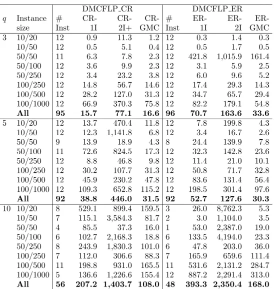
For each problem, the results have been separated into two groups: instances that have been
solved to optimality by all formulations and instances where at least one formulation could not
prove optimality within the given time limit. Table 2 summarizes the results for the instances that
have been solved to optimality within the given time limit of six hours by all formulations for each
problem. The table reports the number of instances that have been solved to optimality, as well
as the average computation times to solve the instances for each of the formulations. For both
problem variants, we observe that the 2I formulation performs worst. Among the 1I and the GMC
based formulations, the GMC based models provide substantially better results.
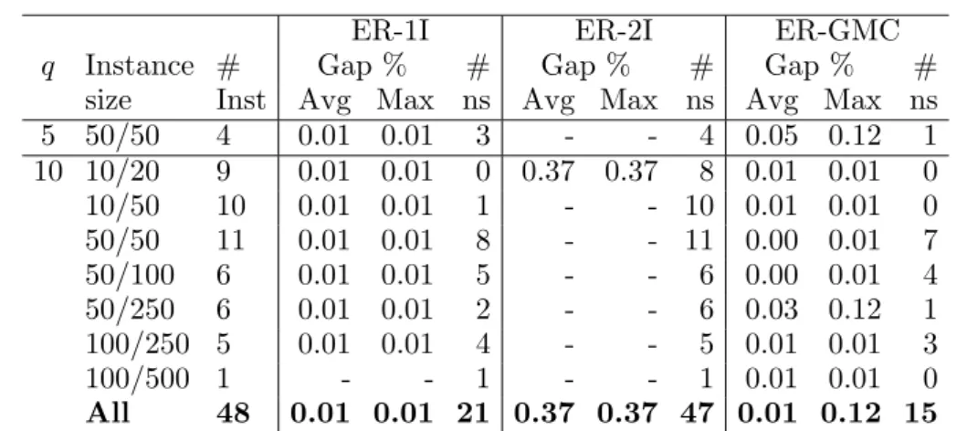
Tables 3 and 4 summarize the results for instances where at least one of the formulations did
not solve the instances in the given time limit. The tables show average and maximum optimality
DMCFLP CR DMCFLP ER
q Instance # CR- CR- CR- # ER- ER-
ER-size Inst 1I 2I+ GMC Inst 1I 2I GMC
3 10/20 12 0.9 11.3 1.2 12 0.3 1.4 0.3
10/50 12 0.5 5.1 0.4 12 0.5 1.7 0.5
50/50 11 6.3 7.8 2.3 12 421.8 1,015.9 161.4
50/100 12 3.6 9.9 2.3 12 3.1 5.9 2.5
50/250 12 3.4 23.2 3.8 12 6.0 9.6 5.2
100/250 12 14.8 56.7 14.6 12 17.4 29.3 14.3
100/500 12 28.2 127.0 31.3 12 34.7 65.7 29.4
100/1000 12 66.9 370.3 75.8 12 82.2 179.1 54.8
All 95 15.7 77.1 16.6 96 70.7 163.6 33.6
5 10/20 12 13.7 470.4 11.8 12 7.8 199.8 4.3
10/50 12 12.3 1,141.8 6.8 12 3.4 16.7 2.6
50/50 9 13.9 18.9 4.3 8 24.4 139.9 7.8
50/100 11 72.6 824.5 17.3 12 32.3 142.8 23.6
50/250 12 8.8 46.8 9.8 12 11.4 21.0 10.1
100/250 12 30.2 107.7 31.3 12 50.8 71.7 32.8
100/500 12 45.9 230.2 47.8 12 83.6 131.4 56.4
100/1000 12 109.3 652.8 115.2 12 198.5 301.4 97.6
All 92 38.8 446.0 31.5 92 52.7 127.6 30.3
10 10/20 8 529.1 899.4 159.5 3 26.0 8,762.3 5.3
10/50 7 115.1 3,584.3 81.7 2 3.0 1,104.0 3.5
50/50 4 85.5 37.3 16.0 1 53.0 2,387.0 19.0
50/100 6 102.7 2,168.3 18.8 6 133.5 4,194.0 23.3
50/250 8 243.9 1,830.3 101.0 6 47.8 203.0 36.0
100/250 7 112.0 306.6 88.3 7 165.9 659.6 111.4
100/500 11 198.8 931.0 165.5 11 531.6 2,131.2 284.7
100/1000 5 136.6 1,226.6 155.4 12 887.2 2,291.4 313.0
All 56 207.2 1,403.7 108.0 48 393.3 2,350.4 168.0
Table 2 CPLEX branch-and-cut computation times (in seconds) for instances solved to optimality by all
formulations for each problem.
CR-1I CR-2I+ CR-GMC
q Instance # Gap % # Gap % # Gap % #
size Inst Avg Max ns Avg Max ns Avg Max ns
3 50/50 1 0.01 0.01 0 0.06 0.06 0 0.01 0.01 0
5 50/50 3 0.12 0.12 2 - - 3 0.01 0.01 2
50/100 1 0.01 0.01 0 0.02 0.02 0 0.01 0.01 0
10 10/20 4 0.05 0.13 1 0.63 0.63 3 0.12 0.31 0
10/50 5 0.01 0.01 2 0.45 0.45 4 0.01 0.01 2
50/50 8 0.10 0.10 7 0.01 0.01 7 0.01 0.01 6
50/100 6 0.01 0.01 5 - - 6 0.01 0.01 5
50/250 4 0.01 0.01 3 - - 4 0.00 0.01 2
100/250 5 0.04 0.04 4 - - 5 0.01 0.01 3
100/500 1 0.01 0.01 0 - - 1 0.01 0.01 0
100/1000 7 0.00 0.00 0 - - 7 0.00 0.01 0
All 40 0.02 0.13 22 0.37 0.63 37 0.03 0.31 18
ER-1I ER-2I ER-GMC
q Instance # Gap % # Gap % # Gap % #
size Inst Avg Max ns Avg Max ns Avg Max ns
5 50/50 4 0.01 0.01 3 - - 4 0.05 0.12 1
10 10/20 9 0.01 0.01 0 0.37 0.37 8 0.01 0.01 0
10/50 10 0.01 0.01 1 - - 10 0.01 0.01 0
50/50 11 0.01 0.01 8 - - 11 0.00 0.01 7
50/100 6 0.01 0.01 5 - - 6 0.00 0.01 4
50/250 6 0.01 0.01 2 - - 6 0.03 0.12 1
100/250 5 0.01 0.01 4 - - 5 0.01 0.01 3
100/500 1 - - 1 - - 1 0.01 0.01 0
All 48 0.01 0.01 21 0.37 0.37 47 0.01 0.12 15
Table 4 CPLEX branch-and-cut optimality gaps for instances of the DMCFLP ER not solved within 6hs.
not been found within the given time limit (#ns). Note that a positive optimality gap indicates
that an optimal solution (i.e., the one with the cut-off value) has been found, but optimality has
not been proven. Forq= 3 andq= 5, a few instances with 50 facility locations have been found to
be difficult to solve. All other instances are for q= 10. Again, the 2I formulations perform worst,
having the highest number of instances where the optimal solution has not been found. For both
problem variants, the GMC finds more solutions than the 1I and 2I formulations. If the optimal
solutions are found, the optimality gaps are low for all three formulations.
5.2.2. Optimization with CPLEX Default Settings
As shown in the previous section, the GMC based formulation outperforms the 1I and 2I
formula-tions for both problem variants in a traditional branch-and-cut environment, allowing for a clear
comparison of the formulations without the interference of heuristics. In practice, however, the
objective is most often to find high quality solutions in short computing times. CPLEX
incorpo-rates several heuristics to find good quality solutions early in the search tree. We now compare
the different formulations using CPLEX with default settings, making full use of the heuristic
capabilities of the MIP solver.
Computational experiments on the same set of test instances indicate trends similar to those
observed in the experiments of Section 5.2.1. The results for the instances that have been solved
by all formulations for each problem are summarized in Table 5. The table reports the number of
DMCFLP CR DMCFLP ER
q Instance # CR- CR- CR- # ER- ER-
ER-size Inst 1I 2I+ GMC Inst 1I 2I GMC
3 10/20 12 1.1 5.7 1.5 12 0.3 1.4 0.3
10/50 12 0.8 3.8 1.2 12 0.5 1.6 1.1
50/50 12 121.8 158.4 18.3 12 302.4 1,402.6 116.2
50/100 12 4.2 13.4 3.3 12 4.8 7.3 3.7
50/250 12 4.3 25.3 5.6 12 7.5 12.3 6.8
100/250 12 13.9 70.0 20.4 12 22.7 36.6 19.1
100/500 12 36.5 155.0 36.3 12 45.9 75.5 36.8
100/1000 12 76.3 440.4 89.3 12 92.7 156.0 64.4
All 96 32.4 109.0 22.0 96 59.6 211.7 31.0
5 10/20 12 10.2 43.0 10.4 12 7.3 42.3 5.8
10/50 12 10.8 121.2 12.9 12 5.0 25.1 5.0
50/50 10 194.6 176.1 62.0 9 663.0 2,126.3 84.2
50/100 12 447.9 518.8 143.3 12 84.6 161.8 35.3
50/250 12 10.2 51.8 11.7 12 14.8 29.2 13.8
100/250 12 40.3 136.5 41.1 12 61.1 104.4 46.0
100/500 12 65.3 270.9 56.1 12 119.5 160.3 69.5
100/1000 12 128.1 741.3 143.4 12 192.8 331.8 126.8
All 94 111.7 259.2 60.1 93 126.8 316.1 47.1
10 10/20 8 59.8 903.8 52.9 8 55.0 2,808.0 10.9
10/50 7 119.3 1,033.6 108.3 8 180.9 4,310.8 28.6
50/50 5 184.4 61.6 44.4 5 392.0 2,946.4 67.0
50/100 7 744.1 1,595.0 97.4 7 577.0 3,186.6 162.1
50/250 10 1,824.1 2,018.3 289.4 9 1,747.9 4,865.4 257.2
100/250 8 2,009.1 1,049.3 503.8 7 258.3 963.0 125.6
100/500 11 208.0 701.5 215.3 11 806.2 3,565.6 416.9
100/1000 8 420.3 1,760.5 355.8 12 957.1 2,809.6 389.8
All 64 740.8 1,192.4 222.2 67 683.3 3,245.6 212.6
Table 5 Computation times (in seconds) using CPLEX with default settings for instances solved to optimality
by all formulations for each problem.
CR-1I CR-2I+ CR-GMC
q Instance # Gap % # Gap % # Gap % #
size Inst Avg Max ns Avg Max ns Avg Max ns
5 50/50 2 0.99 1.18 0 1.17 1.32 0 0.18 0.35 0
10 10/20 4 0.01 0.01 0 0.72 0.96 0 0.01 0.01 0
10/50 5 0.12 0.56 0 0.56 1.36 0 0.26 0.87 0
50/50 7 1.85 3.73 0 1.46 4.21 0 1.36 3.42 0
50/100 5 1.14 2.54 0 0.87 1.84 0 0.58 1.43 0
50/250 2 0.59 0.85 0 0.59 0.89 0 0.42 0.75 0
100/250 4 1.10 2.76 0 0.67 1.61 0 0.69 1.69 0
100/500 1 0.01 0.01 0 0.04 0.04 0 0.01 0.01 0
100/1000 4 0.00 0.00 0 - - 4 0.00 0.01 0
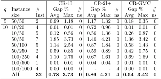
All 32 0.78 3.73 0 0.86 4.21 4 0.54 3.42 0
Table 6 Optimality gaps using CPLEX with default settings for instances of the DMCFLP CR not solved
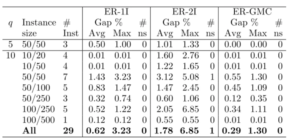
ER-1I ER-2I ER-GMC
q Instance # Gap % # Gap % # Gap % #
size Inst Avg Max ns Avg Max ns Avg Max ns
5 50/50 3 0.50 1.00 0 1.01 1.33 0 0.00 0.00 0
10 10/20 4 0.01 0.01 0 1.60 2.76 0 0.01 0.01 0
10/50 4 0.01 0.01 0 1.22 1.65 0 0.01 0.01 0
50/50 7 1.43 3.23 0 3.12 5.08 1 0.55 1.30 0
50/100 5 0.83 1.47 0 1.47 2.45 0 0.45 1.09 0
50/250 3 0.32 0.74 0 0.60 1.06 0 0.12 0.35 0
100/250 5 0.52 1.22 0 2.05 6.85 0 0.34 1.11 0
100/500 1 0.12 0.12 0 0.55 0.55 0 0.01 0.01 0
All 29 0.62 3.23 0 1.78 6.85 1 0.29 1.30 0
Table 7 Optimality gaps using CPLEX with default settings for instances of the DMCFLP ER not solved within
6hs.
instances for each of the formulations. As in the previous experiments, the 2I formulation performs
worst. Among the 1I and the GMC based formulations, the GMC based models are solved in
substantially shorter computing times.
Tables 6 and 7 summarize the results for instances where at least one of the formulations did
not solve the instances in the given time limit. The tables report average and maximum optimality
gaps as reported by CPLEX, as well as the number of instances where no feasible solution has been
found (#ns). Forq= 5, the few instances that have been found to be difficult to solve are those with
50 facility locations. All other instances are for q= 10. Again, the 2I formulations perform worst.
For some of the instances, the formulation did not find any feasible solution. The GMC formulation
performs similar to the 1I formulation for the DMCFLP CR and presents slightly better results
than the 1I formulation for the DMCFLP ER.
5.3. Closing and Reopening with Capacity Expansion and Reduction
The two problem variants treated above consider either facility closing/reopening or capacity
expansion/reduction. Experiments have also been performed for a third problem variant
combin-ing both features, referred to as the DMCFLP CRER. The problem is modeled by the use of the
DFLPG by using the transition arcs for both problems as shown in Section 3.2. Additionally, arcs
are added representing combined decisions such as facility reopening with subsequent capacity
Alternatively, a specialized flow formulation can be used with two types of flow constraints: one
to manage the capacity of open facilities and one to manage the capacity of closed facilities. The
advantage of the GMC model for this variant is even more obvious than what was observed for the
DMCFLP ER. We proved that the GMC based model provides a stronger LP relaxation than the
specialized flow formulation. Computationally, the average integrality gap (for all instances with
q= 10) improved from 6.00% to 1.06% when using the GMC based model instead of the specialized
formulation. In the traditional branch-and-cut environment, using CPLEX without heuristics and
providing it with the optimal integer solution value as cut-off, the flow formulation takes on average
1,820 seconds to solve the instances of size q= 10, while the GMC based formulation solves the
same instances in an average time of only 206 seconds, about nine times faster. Using CPLEX
default settings, the dominance of the GMC based formulation is mainly preserved. The average
computation time improves from 1,924 to 313 seconds.
5.4. Solution Structure and Instance Properties
We now analyze the structure of the optimal or near-optimal solutions. Figure 2 illustrates for
each problem variant and problem size (10, 50 and 100 candidate facility locations) the minimum
(Min), maximum (Max) and average number (Avg) of selected facility locations. Since a facility
may not be available in all of the subsequent time periods after its construction, a second average
value (Avg open) indicates the average number of facilities that are available (i.e., having `≥1)
at each time period. The results are surprisingly similar for the three problem variants CR, ER
and CRER. On average, about half of the candidate locations have been selected. These facilities
are active only in about two thirds of the planning horizon. For the CR, this is done by closing a
facility. For the ER, the capacity is reduced to level 0.
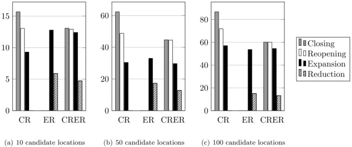
Figure 3 shows different indicators of the solutions structure: the average number of facility
closings and reopenings, as well as the average number of capacity expansions and reductions.
It can be observed that the average values for certain indicators such as capacity expansion and
CR ER CRER 4
6 8 10
(a) 10 candidate locations
CR ER CRER
10 20 30 40 50
(b) 50 candidate locations
CR ER CRER
20 40 60 80 100
(c) 100 candidate locations
l Min
m Max
Avg Avg open
Figure 2 Structure of optimal solutions: minimum, average and maximum number of selected facility locations,
as well as the average number of open facilities per time period throughout the entire planning horizon.
CR ER CRER
0 5 10 15
(a) 10 candidate locations
CR ER CRER
0 20 40 60
(b) 50 candidate locations
CR ER CRER
0 20 40 60 80
(c) 100 candidate locations
Closing Reopening Expansion Reduction
Figure 3 Structure of optimal solutions: average number of facility closings and reopenings, as well as capacity
reductions and expansions.
that the main driver to adjust capacities are high maintenance costs and therefore high quality
solutions tend to provide a total capacity that only slightly exceeds the total demand.
However, an analysis of the solutions for smaller instances reveals that the selected opening
schedules are very different for the three problem variants when the original transportation costs
are used. In contrast, the opening schedules are very similar when the transportation costs are set
struc-ture. The table shows, for each of the indicators, the average number of occurrences in instances
with the original transportation costs and in instances where the transportation costs are set five
times higher. In the same way, it indicates the number of occurrences in instances with regular
demand distribution and with irregular demand distribution. The impact of these instance
prop-erties has been found to be very similar for all three problem variants and is here exemplified
for the DMCFLP CRER, showing the average values over all instances. We can identify a clear
trend. Solutions for instances with original transportation costs involve only a few operations that
adjust the capacities throughout the planning horizon and therefore tend to serve the demand
from a similar set of facility locations. Solutions for instances with high transportation costs
pro-vide capacities that tend to geographically follow the demand along time, constructing on average
more than twice the number of facilities and performing two to three times the operations that
adjust capacities along time. As in both cases the maintenance costs are the same, the motivating
factor to geographically shift capacity is rather given by high transportation costs and the effort
to bring capacities closer to the demand. Regarding the demand distribution, an irregular demand
distribution results in only slightly more capacity adjustments than a regular demand distribution.
Transportation costs Demand distribution
# original 5×higher regular irregular
Constructions 21.7 44.9 33.3 33.3
Closings 21.0 63.3 40.3 43.9
Reopenings 21.0 63.2 40.3 43.8
Capacity expansions 22.3 46.3 33.8 34.7
Capacity reductions 5.3 16.4 10.6 11.1
Avg. open facilities 16.2 28.4 23.2 21.3
Table 8 Impact of instance characteristics (transportation costs and demand distribution) on the solution
structure for the DMCFLP CRER.
Impact on problem difficulty. The instance characteristics not only impact the solution structure,
but also the difficulty of solving the problem. The computing time for instances with irregular total
customer demand is, on average, 30% lower than for instances where the total customer demand is
regular at each time period. In contrast, the ratio between transportation and facility construction
the original transportation costs are, on average, solved around 60 times faster. This is directly
linked to the integrality gap for those instances, which is significantly lower if the ratio between
facility construction and transportation costs is not close to 1.
|T|= 6 |T|= 8 |T|= 10 |T|= 12 |T|= 14
Gap Time Gap Time Gap Time Gap Time Gap Time
% (sec) % (sec) % (sec) % (sec) % (sec)
10/20 0.00 112.1 0.01 180.8 0.01 140.0 0.01 940.7 0.01 2,569.4
10/50 0.00 73.0 0.01 129.1 0.01 302.4 0.01 1,822.0 0.06 6,203.6
50/50 0.17 7,842.3 0.25 8,818.4 0.45 10,820.0 1.23 10,913.3 0.96 12,800.9 50/100 0.02 2,126.8 0.11 4,107.6 0.17 4,201.6 0.56 7,582.8 0.40 9,225.2 50/250 0.01 446.0 0.02 2,002.3 0.01 1,945.0 0.14 7,304.1 0.12 5,655.8 100/250 0.05 2,883.7 0.08 5,516.9 0.14 6,940.4 0.57 8,899.3 0.31 9,481.0
100/500 0.00 339.3 0.00 988.9 0.00 940.8 0.01 2,687.5 0.01 2,571.3
100/1000 0.00 414.5 0.00 463.9 0.00 538.4 0.00 690.2 0.00 549.1
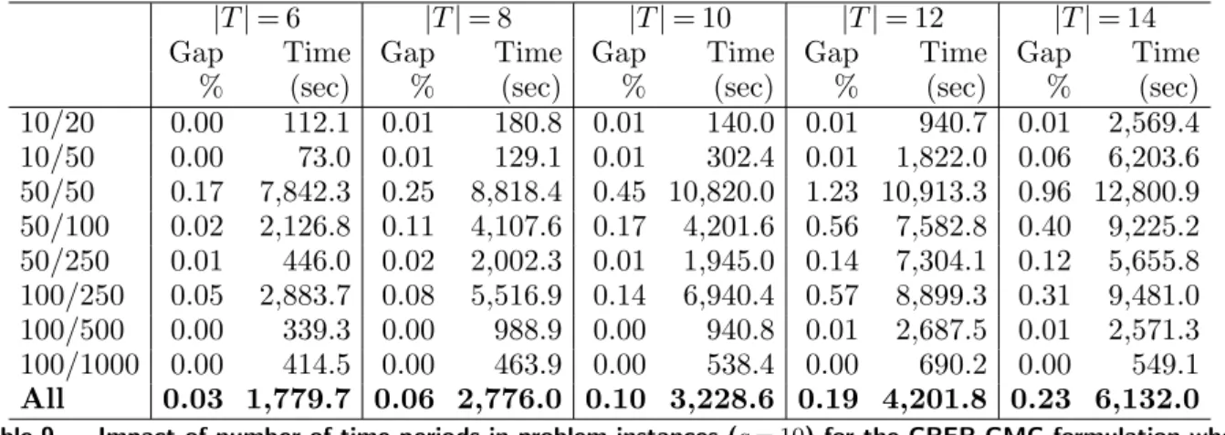
All 0.03 1,779.7 0.06 2,776.0 0.10 3,228.6 0.19 4,201.8 0.23 6,132.0
Table 9 Impact of number of time periods in problem instances (q= 10) for the CRER-GMC formulation when
using CPLEX with default settings.
Finally, we also analyzed the impact of the length of the planning horizon in the problem
instances, using CPLEX with its default settings. For this purpose, instances have also been
generated with different numbers of time periods such that |T| ∈ {6,8,10,12,14}. Table 9
summarizes the average computation times and average optimality gaps for the CRER-GMC
formulation. The computational results are presented for five different numbers of time periods
|T|: 6, 8, 10, 12 and 14. The results are very consistent, showing that the difficulty of the problems
increases proportionally to the number of time periods. For the CRER-1I formulation, a similar
trend was observed. However, the CRER-1I was clearly outperformed by the CRER-GMC for all
tested lengths of the planning horizon.
6.
Conclusions and Future Research
We have introduced a new general facility location problem that unifies several existing
multi-period facility location problems. We showed the flexibility of this generalization by focusing on two
we also reported results on a variant that combines both of these features. For the two first cases, we
derived specialized models based on two well-known formulation approaches. We formally proved
that, even though our model is more general, it provides LP relaxation bounds as strong as the
other formulations for the case of facility closing/reopening and stronger LP relaxation bounds
than the formulations for the other two cases. Computational experiments showed that, for the
two variants involving capacity expansion and reduction, the integrality gap of our model is up to
seven times smaller than the integrality gaps of the specialized formulations. When assessing the
performance of the models in a traditional branch-and-cut environment, the GMC based models
solved the instances, on average, up to nine times faster than the specialized formulations. Using
CPLEX default settings to solve the problem, the GMC based models are, on average, up to six
times faster.
The general model may also be used to model other problem variants not addressed in this work,
e.g., the closing and reopening model of Chardaire et al. (1996) or the dynamic location problem
of Sridharan (1995). In addition, problem variants that involve capacity changes may benefit
from the proposed modeling technique to strengthen the existing models. Problems such as those
presented by Shulman (1991) and Correia and Captivo (2003) can be modeled by the DFLPG
when adding individual constraints such as minimum production bounds for the facilities. Finally,
as the general model is already very strong, it may also be an ideal candidate for decomposition
techniques such as Lagrangian relaxation to find good quality solutions in short computation
times.
Acknowledgements
The authors are grateful to MITACS, the Natural Sciences and Engineering Research Council of
Canada (NSERC) and the Fonds de recherche du Qu´ebec Nature et Technologies for their financial
support. We also thank three anonymous referees for their valuable comments which have helped
References
Arabani, A. B., R. Z. Farahani. 2011. Facility Location Dynamics: An Overview of Classifications and
Applications. Computers & Industrial Engineering 62(1) 408–420.
Behmardi, B., S. Lee. 2008. Dynamic Multi-commodity Capacitated Facility Location Problem in Supply
Chain. Proceedings of the 2008 Industrial Engineering Research Conference. 1914–1919.
Brotcorne, L., G. Laporte, F. Semet. 2003. Ambulance location and relocation models. European Journal of
Operational Research 147(3) 451–463.
Canel, Cem, B. M. Khumawala, J. Law, A. Loh. 2001. An Algorithm for the Capacitated, Multi-Commodity
Multi-Period Facility Location Problem. Computers & Operations Research 28(5) 411–427.
Chardaire, P., A. Sutter, M.-C. Costa. 1996. Solving the dynamic facility location problem. Networks 28(2)
117–124.
Correia, I., M. E. Captivo. 2003. A Lagrangean heuristic for a modular capacitated location problem.Annals
of Operations Research 122141–161.
Correia, I., L. Gouveia, F. Saldanha-da Gama. 2010. Discretized formulations for capacitated location
problems with modular distribution costs.European Journal of Operational Research 204(2) 237–244.
Daskin, M. S. 2008. What you should know about location modeling. Naval Research Logistics 55(4)
283–294.
Dias, J., M. E. Captivo, J. Cl´ımaco. 2006. Capacitated dynamic location problems with opening, closure
and reopening of facilities. IMA Journal of Management Mathematics 17(4) 317–348.
Dias, J., M. E. Captivo, J. Cl´ımaco. 2007. Dynamic Location Problems with Discrete Expansion and
Reduc-tion Sizes of Available Capacities. Investiga¸c˜ao Operacional 27(2) 107–130.
Farahani, R. Z., M. Hekmatfar, eds. 2009.Facility Location - Concepts, Models, Algorithms and Case Studies.
Contributions to Management Science, Physica-Verlag HD, Heidelberg.
Gendron, B., T. G. Crainic. 1994. Relaxations for multicommodity capacitated network design problems.
Tech. rep., Publication CRT-945, Centre de recherche sur les transports, Universit´e de Montr´eal.
Harkness, J. 2003. Facility location with increasing production costs. European Journal of Operational
Research 145(1) 1–13.
Hinojosa, Y., J. Kalcsics, S. Nickel, J. Puerto, S. Velten. 2008. Dynamic supply chain design with inventory.
Computers & Operations Research 35(2) 373–391.
Jacobsen, S. K. 1990. Multiperiod Capacitated Location Models.Discrete Location Theory, chap. 4. 173–208.
Jena, S. D., J.-F. Cordeau, B. Gendron. 2012. Modeling and solving a logging camp location problem.Annals
of Operations Research.doi:10.1007/s10479-012-1278-z.
Klose, A., A. Drexl. 2005. Facility location models for distribution system design. European Journal of
Operational Research 162(1) 4–29.
Luss, H. 1982. Operations Research and Capacity Expansion Problems: A Survey. Operations Research
30(5) 907–947.
Melkote, S., M. S. Daskin. 2001. Capacitated facility location/network design problems. European Journal
of Operational Research 129(3) 481–495.
Melo, M. T., S. Nickel, F. Saldanha-da Gama. 2006. Dynamic multi-commodity capacitated facility location:
a mathematical modeling framework for strategic supply chain planning. Computers & Operations
Research 33(1) 181–208.
Melo, M. T., S. Nickel, F. Saldanha-da Gama. 2009. Facility location and supply chain management A
review. European Journal of Operational Research 196(2) 401–412.
Owen, S. H., M. S. Daskin. 1998. Strategic facility location: A review. European Journal of Operational
Research 111(3) 423–447.
Peeters, D., A. P. Antunes. 2001. On solving complex multi-period location models using simulated annealing.
European Journal of Operational Research 130(1) 190–201.
Shulman, A. 1991. An Algorithm for Solving Dynamic Capacitated Plant Location Problems with Discrete
Expansion Sizes. Operations Research 39(3) 423–436.
Sridharan, R. 1995. The capacitated plant location problem. European Journal of Operational Research
Troncoso, J., R. Garrido. 2005. Forestry production and logistics planning: an analysis using mixed-integer
programming. Forest Policy and Economics 7(4) 625–633.
Van Roy, T. J., D. Erlenkotter. 1982. A Dual-Based Procedure for Dynamic Facility Location. Management
Science 28(10) 1091–1105.
Wesolowsky, G. O., W. G. Truscott. 1975. The Multiperiod Location-Allocation Problem with Relocation
of Facilities. Management Science 22(1) 57–65.
Wu, L., X. Zhang, J. Zhang. 2006. Capacitated facility location problem with general setup cost. Computers