Decision trees: Amelioration, simulation, application

(1)

Master’s Thesis Methodology and Statistics Master Methodology and Statistics Unit, Institute of Psychology,

Faculty of Social and Behavioral Sciences, Leiden University

Date: August 2018

Student number: 1754378

Supervisor: Dr. Dusseldorp

Decision Trees:

Amelioration, Simulation, Application

Master’s Thesis

(2)

(3)

(4)

(5)

(6)

(7)

(8)

(9)

(10)

(11)

(12)

(13)

(14)

(15)

(16)

(17)

(18)

(19)

(20)

(21)

(22)

(23)

(24)

(25)

Decision Trees: Amelioration, Simulation, Application 21

samples were used, and in pruning the tree, the one-standard-error pruning rule is used. To

test the difference in means of the two groups in each leaf of the pruned tree, independent

t-tests were performed. Since the significance level of the t-t-tests are inflated, bias-corrected

effect sizes in the leaves are given. These were estimated using a validation procedure for

small data sets found in QUINT.

Results

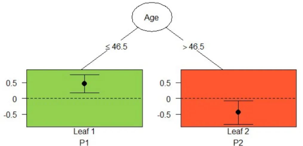
Trees with criterium Effect size. The qualitative interaction tree for the social environmental intervention is a pruned tree with two leaves. The variable “Age” is the

splitting variable with a split point of 46.5 years. Figure 11 displays the tree.

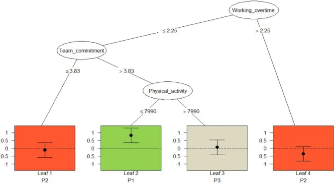
The qualitative interaction tree for the physical environmental intervention is a pruned

tree with two leaves. The variable “Working overtime” is the splitting variable with a split

point of 2.25 hours. Figure 12 displays the tree. Table 3 gives the descriptive statistics of the

Table 3

Descriptive statistics in the leaves of the results for QUINT (version 2.0) for the social environmental intervention (SEI; Figure 11) and the physical environmental intervention (PEI; Figure 12).

n Mean SD n Mean SD

Difference in means (95 % CI)

Bias-corrected effect size d

Fig. 4 SEI+ _SEI-

Leaf 1 90 8.29 22.27 107 -2.23 23.20 10.52

(4.12, 16.92)**

0.31 Leaf 2 59 -3.00 28.22 56 7.66 17.89 10.66

(-19.35, -1.96)*

-0.27 Fig. 5 PEI+ _PEI-

(26)

former trees. Comparing this table to Table 3 from Formanoy et al. (2016) shows that the

results for trees with the difference in means criterium are the same for QUINT (version 2.0)

as for QUINT (version 1.2).

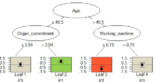
Trees with criterium Difference in means. The qualitative interaction tree for social environmental intervention is a pruned tree with four leaves. The variable “Age” is the first

splitting variable with a split point of 46.5 years, the variables “Organizational commitment”

and “Working overtime” are the second and third splitting variables with split points of 3.94

and 0.75 hours respectively (see Figure 13).

The qualitative interaction tree for physical environmental intervention is a pruned tree

with four leaves. The variable “Working overtime” is the first splitting variable with a split

point of 2.25 hours, the variables “Team commitment” and “Physical activity” are the second

and third splitting variables with split points of 3.83 and 7990 minutes respectively (see

Figure 14). Figure 7 and 8 are the same as Figure 3 and 4 of Formanoy et al. (2016). QUINT

(version 2.0) thus returns the same results as QUINT (version 1.2). Contrary to QUINT

(version 1.2), QUINT (version 2.0) also returns a tree when a minimum effect size of 0.30 is

used.

(27)

Figure 12. Pruned tree with splitting variable Working overtime and a split point at 2.25 hours. Office workers who work fewer hours overtime (≤ 2.25) have a better outcome with the physical environmental intervention than without the physical environmental

intervention (Leaf 1) and those who work more hours overtime (> 2.25) have a worse outcome with the physical environmental intervention than without (Leaf 2). The criterium used in this tree is the effect size.

Figure 13. Pruned tree with splitting variables Age, Organizational commitment and

Working overtime and split points at 46.5 years, 3.94 and 0.75 hours. Office workers younger than 46.5 and committed to the organization benefit from the social environmental

(28)

Discussion

In this paper, QUINT is adapted with the aim to improve its Type II error rate. Subsequently,

a simulation study is used to compare the new version, QUINT (version 2.0), to MOB on

several criteria. The measures of evaluation are the proportion of patients correctly assigned,

the Type I error rate and the Type II error rate. Ultimately, an application study is done to

compare the subgroups that are found by QUINT (version 2.0) to the subgroups that are found

by QUINT (version 1.2). The next paragraphs present the main findings of the simulation and

the application study.

(29)

Findings

To provide an answer to the first research question, the proportion of patients assigned to the

best treatment by QUINT (version 2.0) is compared to the proportion correctly assigned by

MOB. As it turns out, whether there is a difference between the two methods depends upon

the calculation of the proportion correctly assigned by QUINT. QUINT can assign patients to

a subgroup that is indifferent to the assigned treatment alternative. One possibility is to

consider this class incorrectly assigned. A second possibility is to consider this class correctly

assigned. Using the first operationalization, MOB performs better than QUINT. This result

can also be found in earlier studies that compared the methods to each other (Sies & Van

Mechelen, 2016; Van der Geest, 2017). However, whereas other studies use this

operationalization without second thought, it is not so straightforward how the proportion

correctly assigned by QUINT should be calculated. While the first calculation takes into

account that the worst treatment alternative is not ruled out as a possible treatment, the second

calculation takes into account that the best treatment alternative is not ruled out as a possible

treatment. Using the last operationalization, part of the difference between MOB and QUINT

is accounted for by the interaction between method and scenario. This result can be found in

earlier studies as well (Sies & Van Mechelen, 2016; Van der Geest, 2017). Either way the

answer to the research question is not affected by the adaptation of QUINT. If we average the

results of both operationalizations, QUINT and MOB do not differ in the proportion of

patients assigned to the best treatment.

The second research question concerns the Type I error rate and Type II error rate of

QUINT (version 2.0) and MOB. The Type I error rate of QUINT is lower than the Type I

error rate of MOB. These error rates are influenced by interactions between method on one

side and effect size, the number of pre-treatment characteristics and sample size on the other.

(30)

first three results were found earlier (Sies & Van Mechelen, 2016). It should be noted that

Sies and Van Mechelen (2016) used a higher cut-off value for the effect size. Using the same

cut-off value in this study means the third and fourth result would not be present.

The Type I error rate of QUINT is much higher in the present study than in the pilot

study (Van der Geest, 2017). The reverse is true for MOB. Since the Type I error rate is

different for QUINT as well as for MOB it is highly likely that this is due to differences in the

simulation design, i.e. smaller sample sizes and more iterations, rather than the adaptation of

QUINT. Although the Type I error rate of QUINT is high, Dusseldorp and Van Mechelen

(2014) show that this kind of error rate is to be expected with a medium- or large-sized effect

size and a small sample size.

The Type II error rate is influenced by the interaction between method and sample

size. This is in line with earlier research (Sies & Van Mechelen, 2016). There is no substantial

difference between the Type II error rate of QUINT and the Type II error rate of MOB. This

contrasts with findings from earlier research (Sies & Van Mechelen, 2016; Van der Geest,

2017). The Type II error rate (0.216) of QUINT (version 2.0) is clearly lower than the Type II

error rate (0.776) of QUINT (version 1.2) as found in the pilot study. Since the sample sizes

in the simulation study differ, direct comparison of the overall Type II error rate of QUINT is

not appropriate, however. Both simulations do have Type II error rates for datasets consisting

of 300 cases. With this sample size QUINT (version 2.0) still has a much lower Type II error

rate than QUINT (version 1.2) (0.265 versus 0.717). The Type II error rate is changed for the

better by the adaptation.

The third research question is answered by comparing the application of QUINT

(version 2.0) to the application of QUINT (version 1.2) on data used in Formanoy et al.

(2016). When the partitioning criterion is effect size, both versions of QUINT result in the

(31)

to return a tree for the physical environmental intervention when in fact there is a qualitative

interaction. QUINT (version 2.0) does return a tree in this situation. In this respect QUINT

(version 2.0) is better. The application shows QUINT (version 2.0) is at least as good as

QUINT (version 1.2).

Limitation

Although it seems like QUINT (version 2.0) is better than QUINT (version 1.2), the sample

sizes currently used to study the effectiveness of QUINT (version 2.0) are rather small. Earlier

studies have used sample sizes of 300 and 1000 (Sies & Van Mechelen, 2016; Van der Geest,

2017), whereas the present study uses sample sizes of 150 and 300. Using larger sample sizes

could shed more light on the (acceptability of) the Type I error rate of QUINT (version 2.0).

Future research

Future research could expand the present study by adding an extra evaluation criterion. Sies

and Van Mechelen (2016) used an evaluation criterion that takes into account the expected

outcome that patients theoretically could have achieved when all patients receive their optimal

treatment. To achieve this, the benefit of administering the treatments based on the decision

trees over administering the overall best treatment is divided by the benefit of administrating

each patient their optimal treatment over administering the overall best treatment. This

criterion might be the most relevant criterion to the patient himself.

Another issue for future research is the method(s) used to compare QUINT to. MOB is

a tree-based method, but not a method specifically designed to search for treatment-subgroup

interactions. It would be appropriate to compare QUINT to another tree-based method

(32)

Conclusion

The simulation study shows that QUINT (version 2.0) has a lower Type II error rate than

QUINT (version 1.2). The adaptation does not have a negative impact on the proportion good

predicted and the Type I error rate. In addition, the application study shows that QUINT

(version 2.0) is at least as competent as QUINT (version 1.2). Clearly, the adaptation of

QUINT appears to be successful.

(33)

References

Albisser, A.M. (2000). The disease management equation. IFAC Proceedings Volumes 33(3),

47-52.

Cohen, J. (1988). Statistical Power Analysis for the Behavioral Sciences. New York:

Routledge.

Dusseldorp, E., Conversano, C., & Van Os, B. J. (2010). Combining an additive and tree-

based regression model simultaneously: Stima. Journal of Computational and

Graphical Statistics, 19(3), 514–530. doi:10.1198/jcgs.2010.06089

Dusseldorp, E., Doove, L., & Van Mechelen, I. (2015). Quint: An R package for

identification of subgroups of clients who differ in which treatment alternative is best for them. Behavior Research Methods.

Dusseldorp, E., & Meulman, J. J. (2004). The regression trunk approach to discover treatment covariate interaction. Psychometrika, 69(3), 355–374.

Dusseldorp, E., & Van Mechelen, I. (2014). Qualitative interaction trees: a tool to identify qualitative treatment–subgroup interactions. Statistics in Medicine, 33(2), 219-237. Epstein, R.S., & Sherwood, L.M. (1996). From outcomes research to disease management: a

guide for the perplexed. Ann Intern Med. 124(9), 832–837.

Formanoy, M. A., Dusseldorp, E., Coffeng, J. K., Van Mechelen, I., Boot, C. R., Hendriksen, I. J., & Tak, E. C. (2016). Physical activity and relaxation in the work setting to reduce the need for recovery: what works for whom? BMC Public Health, 16(1), 866.

Foster, J., Taylor, J., & Ruberg, S. (2011). Subgroup identification from randomized clinical trial data. Statistics in Medicine, 30(24), 2867–2880.

(34)

Peile, E. (2004). Reflections from medical practice: balancing evidence-based practice with practice-based evidence. In R. Pring & G. Thomas (Ed.), Evidence-Based Practice in Education (pp. 102-108). McGraw-Hill Education: London.

Sies, A., & Van Mechelen, I. (2016). Comparing four methods for estimating tree-based treatment regimes. Manuscript in preparation.

Su, X., Tsai, C. L., Wang, H., Nickerson, D. M., & Li, B. (2009). Subgroup analysis via recursive partitioning. The Journal of Machine Learning Research, 10, 141–158. Van der Geest, M. (2017). Simulation study QUINT vs. MOB. Internal Leiden University

Report: unpublished.

Zeileis, A., Hothorn, T., & Hornik, K. (2008). Model-based recursive partitioning. Journal of Computational and Graphical Statistics, 17, 492–514. doi:

(35)

Appendix A: R code quint2()

This appendix shows the code to search for a qualitative interaction tree. Red text is used to highlight code present in quint() but not in quint2() and green text is used to highlight code present in quint2() but not in quint().

quint2<- function(formula, data, control=NULL){ #Dataformat without use of formula:

#dat:data; first column in dataframe = the response variable

#second column in dataframe = the dichotomous treatment vector

#(coded with treatment A=1 and treatment B=2)

#rest of the columns in dataframe are the predictors

#maxl: maximum total number of leaves (terminal nodes) of the final tree :

#Lmax

dat <- as.data.frame(data) if (missing(formula)) { y <- dat[, 1]

tr <- dat[, 2]

Xmat <- dat[, -c(1, 2)] dat <- na.omit(dat)

if (length(levels(as.factor(tr))) != 2) {

stop("Quint cannot be performed. The number of treatment conditions does not equal 2.")

} } else {

F1 <- Formula(formula)

mf1 <- model.frame(F1, data = dat) y <- as.matrix(mf1[, 1])

origtr <- as.factor(mf1[, 2]) tr <- as.numeric(origtr)

if (length(levels(origtr)) != 2) {

stop("Quint cannot be performed. The number of treatment conditions does not equal 2.")

}

Xmat <- mf1[, 3:dim(mf1)[2]] dat <- cbind(y, tr, Xmat) dat <- na.omit(dat)

cat("Treatment variable (T) equals 1 corresponds to", attr(F1, "rhs")[[1]], "=", levels(origtr)[1], "\n") cat("Treatment variable (T) equals 2 corresponds to", attr(F1, "rhs")[[1]], "=", levels(origtr)[2], "\n") names(dat)[1:2] <- names(mf1)[1:2]

}

(36)

N<-length(y)

if(is.null(control)) {

control <- quint.control() #Use default control parameters and criter

ion

}

#specify criterion , parameters a and b (parvec), weights and maximum

#number of leaves:

crit <- control$crit parvec <- control$parvec w <- control$w

maxl <- control$maxl

#if no control argument was specified ,use default parameter values

#Default parameters a1 and a2 for treatment cardinality condition:

if(is.null(parvec)){

a1 <- round(sum(tr==1)/10) a2 <- round(sum(tr==2)/10) parvec <- c(a1, a2)

control$parvec <- parvec }

if(is.null(w)){

#edif=expected mean difference between treatment and control; default

#value for effect size criterion: edif = 3 (=Cohen's d),

#and for difference in means criterion: edif= IQR(Y)

edif <- ifelse(crit=="es", 3, IQR(y)) w1 <- 1/log(1+edif)

#bal= balance (ratio) between "difference in treatment outcomes

#component" and "cardinality component"

w2 <- 1/log(length(y)/2) w <- c(w1, w2)

control$w <- w }

##Create matrix for results

allresults <- matrix(0, nrow=maxl-1, ncol=6) splitpoints <- matrix(0, nrow=maxl-1, ncol=1) ## create a vector for true split points

##Start of the tree growing: all persons are in the rootnode. L=1; #Criterion value (cmax)=0

root <- rep(1, length(y)) cmax <- 0

#Step 1

#Generate design matrix D with admissable assignments after first split

dmat1 <- matrix(c(1,2,2,1), nrow=2)

#Select the optimal triplet for the first split: the triplet resulting i n

#the maximum value of the criterion (critmax1)

(37)

#meant0

rootvec <- c(sum(tr==1), sum(tr==2), mean(y[tr==1])-mean(y[tr==2]))

critmax1 <- bovar(y, Xmat, tr, gm=root, dmatsg=dmat1,

dmatsel=rep(1,nrow(dmat1)), parents=rootvec, parvec, w ,

nsplit=1, crit=crit)

#Make the first split

if(is.factor(Xmat[,critmax1[1]])==FALSE){

Gmat <- makeGchmat(root, Xmat[,critmax1[1]], critmax1[2]) } if(is.factor(Xmat[,critmax1[1]])==TRUE){

possibleSplits <- determineSplits(x=Xmat[,critmax1[1]], gm=root) assigMatrix <- makeCatmat(x=Xmat[,critmax1[1]], gm=root,

z=possibleSplits[[1]], splits=possibleSplits[[2]]) Gmat <- makeGchmatcat(gm=root, splitpoint=critmax1[2], assigMatrix=assigMatrix)

}

cat("split 1","\n") cat("#leaves is 2","\n")

##Keep the child node numbers nnum; #ncol(Gmat) is current number of ##leaves (=number of candidate parentnodes)=L; #ncol(Gmat)+1 is total ##number of leaves after the split (Lafter)

nnum <- c(2,3) L <- ncol(Gmat)

##Keep the results (split information, fit information, end node ##information) after the first split

if(critmax1[4]!=0){

allresults[1,] <- c(1,critmax1[-3]) #Keep the splitpoints

ifelse(is.factor(Xmat[,critmax1[1]])==F, splitpoints[1] <- critmax1[2] ,

splitpoints[1] <- paste(as.vector(unique(

sort(Xmat[Gmat[,1]==1, critmax1[1]]))), collapse=", ")) dmatrow<-dmat1[critmax1[3],]

cmax <- allresults[1, 4]

endinf <- ctmat(Gmat,y,tr,crit=crit) ####changed

} else { ##if there is no optimal triplet for the first split: Gmat <- Gmat*0

dmatrow <- c(0,0)

endinf <- matrix(0, ncol=8, nrow=2) }

##Check the qualitative interaction condition: Cohen's d in the leafs

#after the first split >=dmin qualint <- "Present"

if(abs(endinf[1,7])<control$dmin | abs(endinf[2,7])<control$dmin) { L <- maxl

(38)

both of the effect sizes are lower than absolute value",

control$dmin,". There is no clear qualitative interaction present in the data.","\n")

}

# Return an object of length 1 when C is 0

if (cmax == 0) { object <- 1

print("Quint cannot be performed. C is 0.") class(object) <- "quint"

return(object) } else {

##Perform bias-corrected bootstrapping for the first split: if(control$Boot==TRUE&cmax!=0){

#initiate bootstrap with stratification on treatment groups:

indexboot <- Bootstrap(y, control$B, tr)

critmax1boot <- matrix(0, ncol=6, nrow=control$B)

#initialize matrices to keep results

Gmattrain <- array(0, dim=c(N,maxl,control$B)) Gmattest <- array(0, dim=c(N,maxl,control$B))

allresultsboot <- array(0, dim=c(maxl-1,9,control$B)) #find best first split for the k training sets

for (b in 1:control$B) {

cat("Bootstrap sample ",b,"\n")

##use the bootstrap data as training set critmax1boot[b,]<-

bovar(y[indexboot[,b]],Xmat[indexboot[,b],],

tr[indexboot[,b]],root,dmat1,rep(1,nrow(dmat1)), rootvec,parvec,w,1,crit=crit)

if(is.factor(Xmat[,critmax1boot[b,1]])==FALSE){ Gmattrain[,c(1:2),b]<-

makeGchmat(gm=root, varx=Xmat[indexboot[,b],critmax1boot[b,1]], splitpoint=critmax1boot[b,2])

##use the original data as testset

Gmattest[,c(1:2),b]<-makeGchmat(gm=root,

varx=Xmat[,critmax1boot[b,1]], splitpoint=critmax1boot[b,2]) }

if(is.factor(Xmat[,critmax1boot[b,1]])==TRUE){ possibleSplits <-

determineSplits(x=Xmat[indexboot[,b], critmax1boot[b,1]], gm=root)

assigMatrixTrain <-

makeCatmat(x=Xmat[indexboot[,b], critmax1boot[b,1]], gm=root, z=possibleSplits[[1]], splits=possibleSplits[[2]]) Gmattrain[,c(1:2),b]<-

makeGchmatcat(gm=root, splitpoint=critmax1boot[b,2], assigMatrix=assigMatrixTrain)

(39)

makeCatmat(x=Xmat[,critmax1boot[b,1]], gm=root,

z=possibleSplits[[1]], splits=possibleSplits[[2]]) Gmattest[,c(1:2),b]<-

makeGchmatcat(gm=root, splitpoint=critmax1boot[b,2], assigMatrix=assigMatrixTest)

}

End <- cpmat(Gmattest[,c(1:2),b], y, tr, crit=crit)

#select the right row in the design matrix

dmatsel <- t(dmat1[critmax1boot[b,3],])

allresultsboot[1,c(1:8),b] <- c(1,critmax1boot[b,c(1:2)], computeCtest(End, dmatsel, w)) allresultsboot[1,9,b] <- critmax1boot[b,4]-allresultsboot[1,4,b] if(critmax1boot[b,4]==0) {allresultsboot[1,,b]<-NA}

} }

#Repeat the tree growing procedure

stopc <- 0

while(L<maxl){

cat("current value of C", cmax,"\n") cat("split", L, "\n")

Lafter <- ncol(Gmat)+1

cat("#leaves is", Lafter, "\n")

##make a designmatrix (dmat) for the admissible assignments of the #leaves after the split

dmat <- makedmat(Lafter) dmatsg <- makedmats(dmat)

#make parentnode information matrix, select best observed parent node

#(with optimal triplet)

parent <- cpmat(Gmat,y,tr,crit=crit)

critmax <- bonode(Gmat,y,Xmat,tr,dmatrow,dmatsg,parent,parvec,w,L, crit=crit)

##Perform the best split and keep results if(is.factor(Xmat[,critmax[2]])==FALSE){

Gmatch <- makeGchmat(Gmat[,critmax[1]], Xmat[,critmax[2]], critmax[3])

}

if(is.factor(Xmat[,critmax[2]])==TRUE){

possibleSplits <- determineSplits(x=Xmat[,critmax[2]], gm=Gmat[,critmax[1]])

assigMatrix <- makeCatmat(x=Xmat[,critmax[2]], gm=Gmat[,critmax[1]], z=possibleSplits[[1]],

splits=possibleSplits[[2]])

Gmatch <- makeGchmatcat(gm=Gmat[,critmax[1]], splitpoint=critmax[3], assigMatrix=assigMatrix)

}

Gmatnew <- cbind(Gmat[,-critmax[1]], Gmatch)

(40)

ifelse(is.factor(Xmat[,critmax[2]])==F,

splitpoints[L] <- round(critmax[3], digits = 2), splitpoints[L] <-

paste(as.vector(unique(sort(Xmat[Gmatch[,1]==1,critmax[2]]))) ,

collapse=", ")) dmatrownew <- dmatsg[critmax[4],]

#check if cmax new is higher than current value

if(allresults[L,4]<=cmax){

cat("splitting process stopped after number of leaves equals",L, "because new value of C was not higher than current value of C","\n")

stopc<-1 }

##repeat this procedure for the bootstrap samples if(control$Boot==TRUE & stopc!=1){

critmaxboot<-matrix(0,nrow=control$B,ncol=7) for (b in 1:control$B){

cat("Bootstrap sample ",b,"\n")

#make parentnode information matrix pmat

parent <- cpmat(Gmattrain[,c(1:(Lafter-1)),b], y[indexboot[,b]], tr[indexboot[,b]], crit=crit)

critmaxboot[b,] <-

bonode(Gmat=Gmattrain[,c(1:(Lafter-1)),b], y=y[indexboot[,b]], Xmat=Xmat[indexboot[,b],], tr=tr[indexboot[,b]], dmatrow, dmatsg, parent, parvec, w, nsplit=L, crit=crit)

#best predictor and node of this split for the training samples

if(is.factor(Xmat[,critmaxboot[b,2]])==FALSE){

Gmattrainch <- makeGchmat(Gmattrain[, critmaxboot[b,1],b],

Xmat[indexboot[,b], critmaxboot[b,2]], critmaxboot[b,3])

Gmattestch <- makeGchmat(Gmattest[,critmaxboot[b,1],b], Xmat[, critmaxboot[b,2]],

critmaxboot[b,3]) }

if(is.factor(Xmat[,critmaxboot[b,2]])==TRUE){ possibleSplits <-

determineSplits(x=Xmat[indexboot[,b], critmaxboot[b,2]], gm=Gmattrain[,critmaxboot[b,1],b])

assigMatrixTrain <-

makeCatmat(x=Xmat[indexboot[,b], critmaxboot[b,2]], gm=Gmattrain[,critmaxboot[b,1],b],

z=possibleSplits[[1]], splits=possibleSplits[[2]]) Gmattrainch <- makeGchmatcat(gm=Gmattrain[,critmaxboot[b,1],b], splitpoint=critmaxboot[b,3],

assigMatrix=assigMatrixTrain)

assigMatrixTest <-

makeCatmat(x=Xmat[,critmaxboot[b,2]],

(41)

z=possibleSplits[[1]], splits=possibleSplits[[2]])

Gmattestch <- makeGchmatcat(gm=Gmattest[,critmaxboot[b,1],b], splitpoint=critmaxboot[b,3], assigMatrix=assigMatrixTest) }

Gmattrain[,c(1:Lafter),b] <-

cbind(Gmattrain[,c(1:(Lafter-1))[-critmaxboot[b,1]],b], Gmattrainch)

Gmattest[,c(1:Lafter),b] <-

cbind(Gmattest[,c(1:(Lafter-1))[-critmaxboot[b,1]],b], Gmattestch)

##compute criterion value for the test sets

End <- cpmat(Gmattest[,c(1:Lafter),b],y,tr,crit=crit)

#select the right row in the design matrix

if(critmaxboot[b,5]!=0){

dmatsel<-t(dmatsg[critmaxboot[b,4],]) allresultsboot[L,c(1:8),b] <-

c(nnum[critmaxboot[b,1]],critmaxboot[b,2],critmaxboot[b,3], computeCtest(End, dmatsel, w))

allresultsboot[L,9,b]<-critmaxboot[b,5]-allresultsboot[L,4,b] }

if(critmaxboot[b,5]==0){ allresultsboot[L,,b] <-NA }

}

if(sum(is.na(allresultsboot[L,9,]))/control$B > .10 ){

warning("After split ",L,", the partitioning criterion cannot be computed in more than 10 percent of the bootstrap samples. The split is unstable." )

} }

#update the parameters after the split:

if(stopc==0) { Gmat <- Gmatnew

dmatrow <- dmatrownew cmax <- allresults[L,4] L <- ncol(Gmat)

nnum <- c(nnum[-critmax[1]],nnum[critmax[1]]*2,nnum[critmax[1]]*2+1) } else {L <- maxl}

#end of while loop

}

Lfinal <- ncol(Gmat) #Lfinal=final number of leaves of the tree

#create endnode information of the tree

(42)

endinf[,c(2:9)] <- ctmat(Gmat,y,tr,crit=crit)} ####changed endinf <- data.frame(endinf)

endinf[,10] <- dmatrow endinf[,1] <- nnum index <- leafnum(nnum) endinf <- endinf[index,]

rownames(endinf) <- paste("Leaf ",1:Lfinal,sep="") if(crit == 'es'){ ### this was added/changed

colnames(endinf) <- c("node","#(T=1)", "meanY|T=1", "SD|T=1","#(T=2)", "meanY|T=2","SD|T=2","d", "se", "class")}

if(crit == 'dm'){ ### this was added

colnames(endinf) <- c("node","#(T=1)", "meanY|T=1", "SD|T=1","#(T=2)", "meanY|T=2","SD|T=2","diff", "se", "class")} if(Lfinal==2){allresults <- c(2,allresults[1,])}

if(Lfinal>2){

allresults <- cbind(2:Lfinal, allresults[1:(Lfinal-1),]) }

#compute final estimate of optimism and standard error:

if(control$Boot==TRUE){ #raw mean and sd:

opt <- sapply(1:(Lfinal-1),

function(kk, allresultsboot){mean(allresultsboot[kk,9,], na.rm=TRUE)},

allresultsboot=allresultsboot) se_opt <- sapply(1:(Lfinal-1),

function(kk,allresultsboot){sd(allresultsboot[kk,9,], na.rm=TRUE) /

sqrt(sum(!is.na(allresultsboot[kk,9,])))}, allresultsboot=allresultsboot)

if(Lfinal==2){allresults <- c(allresults[1:5], allresults[5]-opt,opt, se_opt, allresults[6:7])

allresults <- data.frame(t(allresults)) }

if(Lfinal>2){

allresults <- cbind(allresults[,1:5], allresults[,5]-opt,opt, se_opt ,

allresults[,6:7]) allresults <- data.frame(allresults) }

allresults[,3] <- colnames(Xmat)[allresults[,3]] splitnr <- 1:(Lfinal-1)

allresults <- cbind(splitnr, allresults)

colnames(allresults) <- c("split", "#leaves", "parentnode",

"splittingvar", "splitpoint", "apparent", "biascorrected", "opt", "se","compdif", "compcard")

}

if(control$Boot==FALSE){ if(Lfinal>2){

(43)

}

if(Lfinal==2){

allresults <- data.frame(t(allresults)) }

allresults[,3] <- colnames(Xmat)[allresults[,3]] splitnr <- 1:(Lfinal-1)

allresults <- cbind(splitnr, allresults)

colnames(allresults) <- c("split", "#leaves", "parentnode",

"splittingvar", "splitpoint", "apparent", "compdif","compcard")

}

colnames(Gmat) <- nnum

##split information (si): also include childnode numbers si <- allresults[,3:5]

cn <- paste(si[,1]*2, si[,1]*2+1, sep=",")

si <- cbind(parentnode=si[,1], childnodes=cn, si[,2:3], truesplitpoint=splitpoints[1:nrow(si)]) rownames(si) <- paste("Split ", 1:(Lfinal-1), sep="")

if(control$Boot==FALSE){

object <- list(call=match.call(), crit=crit, control=control,

data=dat, si=si, fi=allresults[,c(1:2,6:8)], li=endinf, nind=Gmat[,index])

}

if(control$Boot==TRUE){

nam <- c("parentnode", "splittingvar", "splitpoint", "C_boot", "C_compdif", "checkdif", "C_compcard", "checkcard", "opt")

dimnames(allresultsboot) <- list(NULL, nam, NULL)

object <- list(call = match.call(), crit = crit, control = control, indexboot = indexboot, data = dat, si = si,

fi = allresults[, c(1:2, 6:11)], li = endinf, nind = Gmat[, index], siboot = allresultsboot) }

class(object) <- "quint" return(object)

}

(44)

Appendix B: R code prune.quint2()

This appendix shows the code to prune the qualitative interaction tree. Green text is used to highlight code present in prune.quint2() but not in prune.quint().

prune.quint2 <- function(tree, pp=1,...){ object <- tree

if(length(object) == 1) { besttree <- 1

class(besttree) <- "quint" return(besttree)

} else {

#pp=pruning parameter

if(names(object$fi[4])=="Difcomponent"){

stop("Pruning is not possible; The quint object lacks estimates of t he

biascorrected criterion. Grow again a large tree using the bootstrap procedure." )}

object$fi[is.na(object$fi[,4]),4]<-0 object$fi[is.na(object$fi[,5]),5]<-0

maxrow<-which(object$fi[,4]==max(object$fi[,4]))[1]

if(is.na(object$fi[maxrow,6])) maxrow <- maxrow - 1

bestrow<-min( which(object$fi[,4]>=

(object$fi[maxrow,4]-pp*object$fi[maxrow,6]) ) ) con<-object$control

con$Boot<-FALSE

con$maxl <- bestrow + 1

besttree <- quint2(data = object$data, control = con) besttree$fi <- object$fi[1:bestrow, ]

objboot <- list(siboot = object$siboot[1:bestrow, , ]) besttree <- c(besttree, objboot)

besttree$control$Boot <- object$control$Boot

# Check whether there is a qualitative interaction

if(colnames(besttree$li)[8]=="d"){ # criterium is es

if((any(abs(subset(besttree$li, class == 1, d)) >= con$dmin) & any(abs(subset(besttree$li, class == 2, d)) >= con$dmin)) == FALSE) {

besttree <- 1 }

} else { # criterium is dm

if((any(abs(subset(besttree$li, class == 1, diff) /

(45)

(sum(besttree$li[besttree$li[,10]==1, c(2, 5)]) - 2))) >= con$dmin) &

any(abs(subset(besttree$li, class == 2, diff) /

sqrt(((besttree$li[besttree$li[,10]==2, 2] - 1) * besttree$li[besttree$li[,10]==2, 4] ^ 2 + (besttree$li[besttree$li[,10]==2, 5] - 1) * besttree$li[besttree$li[,10]==2, 7] ^ 2) /

(sum(besttree$li[besttree$li[,10]==2, c(2, 5)]) - 2))) >= con$dmin)) == FALSE) {

besttree <- 1 }

}

class(besttree) <- "quint" return(besttree)

(46)

Appendix C: Example R code for MOB and QUINT

Example code MOB with Pima Indians diabetes data # Load MOB

library(party)

# Load Pima Indians diabetes data

data(PimaIndiansDiabetes2, package = "mlbench")

PimaIndiansDiabetes <- na.omit(PimaIndiansDiabetes2[,-c(4, 5)]) # remove missing values

# Create formula with diabetes as outcome variable

fmPID <- mob(diabetes ~ glucose | pregnant + pressure + mass + pedigree + age, data = PimaIndiansDiabetes, model = glinearModel, family = binomial())

# Visualize the model plot(fmPID)

# Show coefficients and corresponding odds ratios coef(fmPID)

exp(coef(fmPID)[,2])

Example code QUINT with BCRP data # Load QUINT

library(quint)

# Read data into memory data(bcrp)

ex_data <- subset(bcrp, cond < 3) # exclude the control condition

(47)

# Fix the seed set.seed(47)

# Analysis with change score in depression as outcome variable quint1 <- quint(formula1, data = ex_data)

# Give a summary of the analysis summary(quint1)

quint1$fi quint1$si quint1$li

# Prune tree to avoid overfitting quint1pr <- prune(quint1)

# Plot the pruned tree plot(quint1pr)

(48)

Appendix D: Repeated measures ANOVA Proportion good predicted (excl. class 3)

This appendix shows the SPSS table of the within-subjects effects with the proportion good predicted as the dependent variable. Class 3 is considered as predicted incorrectly.

Table D1

Repeated Measures Analysis of Variance of Proportion good predicted with class 3 excluded (Within-Subjects Effects)

Source

Type III Sum of Squares df

Mean

Square F Sig.

Partial Eta Squared

Eta Squared Method Sphericity

Assumed

14.417 1 14.417 982.795 .000 .094 .081

Greenhouse-Geisser

14.417 1.000 14.417 982.795 .000 .094 .081

Huynh-Feldt 14.417 1.000 14.417 982.795 .000 .094 .081 Lower-bound 14.417 1.000 14.417 982.795 .000 .094 .081 Method *

n

Sphericity Assumed

.621 1 .621 42.357 .000 .004 .004

Greenhouse-Geisser

.621 1.000 .621 42.357 .000 .004 .004

Huynh-Feldt .621 1.000 .621 42.357 .000 .004 .004 Lower-bound .621 1.000 .621 42.357 .000 .004 .004 Method *

J

Sphericity Assumed

3.700 1 3.700 252.201 .000 .026 .021

Greenhouse-Geisser

3.700 1.000 3.700 252.201 .000 .026 .021

effect.size

Sphericity Assumed

4.356 1 4.356 296.938 .000 .030 .025

Greenhouse-Geisser

4.356 1.000 4.356 296.938 .000 .030 .025

(49)

Table D1 Continued

Source

Mean

Square F Sig.

Partial Eta Squared Eta Squared Method * rho Sphericity Assumed

.265 2 .133 9.049 .000 .002 .001

Greenhouse-Geisser

.265 2.000 .133 9.049 .000 .002 .001

scenario

Sphericity Assumed

2.180 3 .727 49.527 .000 .015 .012

Greenhouse-Geisser

2.180 3.000 .727 49.527 .000 .015 .012

Huynh-Feldt 2.180 3.000 .727 49.527 .000 .015 .012 Lower-bound 2.180 3.000 .727 49.527 .000 .015 .012 Method *

n * J

Sphericity Assumed

.013 1 .013 .861 .353 .000 .000

Greenhouse-Geisser

.013 1.000 .013 .861 .353 .000 .000

Huynh-Feldt .013 1.000 .013 .861 .353 .000 .000 Lower-bound .013 1.000 .013 .861 .353 .000 .000 Method *

n * effect.size

Sphericity Assumed

.263 1 .263 17.957 .000 .002 .001

Greenhouse-Geisser

.263 1.000 .263 17.957 .000 .002 .001

n * rho

Sphericity Assumed

.010 2 .005 .346 .707 .000 .000

Greenhouse-Geisser

.010 2.000 .005 .346 .707 .000 .000

n * scenario

Sphericity Assumed

6.771 3 2.257 153.853 .000 .046 .038

Greenhouse-Geisser

6.771 3.000 2.257 153.853 .000 .046 .038

(50)

Table D1 Continued

Source

Mean

Square F Sig.

Partial Eta Squared Eta Squared Method *

J * effect.size

Sphericity Assumed

.675 1 .675 46.006 .000 .005 .004

Greenhouse-Geisser

.675 1.000 .675 46.006 .000 .005 .004

J * rho

Sphericity Assumed

.178 2 .089 6.084 .002 .001 .001

Greenhouse-Geisser

.178 2.000 .089 6.084 .002 .001 .001

J * scenario

Sphericity Assumed

.042 3 .014 .954 .413 .000 .000

Greenhouse-Geisser

.042 3.000 .014 .954 .413 .000 .000

effect.size * rho

Sphericity Assumed

.061 2 .031 2.089 .124 .000 .000

Greenhouse-Geisser

.061 2.000 .031 2.089 .124 .000 .000

Huynh-Feldt .061 2.000 .031 2.089 .124 .000 .000 Lower-bound .061 2.000 .031 2.089 .124 .000 .000 Method * effect.size * scenario Sphericity Assumed

2.006 3 .669 45.573 .000 .014 .011

Greenhouse-Geisser

2.006 3.000 .669 45.573 .000 .014 .011

rho * scenario

Sphericity Assumed

.337 6 .056 3.829 .001 .002 .002

Greenhouse-Geisser

.337 6.000 .056 3.829 .001 .002 .002

(51)

Table D1 Continued

Source

Mean

Square F Sig.

n * J * effect.size

Sphericity Assumed

.090 1 .090 6.112 .013 .001 .001

Greenhouse-Geisser

.090 1.000 .090 6.112 .013 .001 .001

n * J * rho

Sphericity Assumed

.031 2 .015 1.056 .348 .000 .000

Greenhouse-Geisser

.031 2.000 .015 1.056 .348 .000 .000

n * J * scenario

Sphericity Assumed

.549 3 .183 12.476 .000 .004 .003

Greenhouse-Geisser

.549 3.000 .183 12.476 .000 .004 .003

n * effect.size * rho

Sphericity Assumed

.020 2 .010 .671 .511 .000 .000

Greenhouse-Geisser

.020 2.000 .010 .671 .511 .000 .000

n * effect.size *

scenario

Sphericity Assumed

.471 3 .157 10.695 .000 .003 .003

Greenhouse-Geisser

.471 3.000 .157 10.695 .000 .003 .003

n * rho *

scenario

Sphericity Assumed

.110 6 .018 1.246 .279 .001 .001

Greenhouse-Geisser

.110 6.000 .018 1.246 .279 .001 .001

(52)

Table D1 Continued

Source

Mean

Square F Sig.

J * effect.size * rho

Sphericity Assumed

.018 2 .009 .600 .549 .000 .000

Greenhouse-Geisser

.018 2.000 .009 .600 .549 .000 .000

J * effect.size *

scenario

Sphericity Assumed

.091 3 .030 2.067 .102 .001 .001

Greenhouse-Geisser

.091 3.000 .030 2.067 .102 .001 .001

J * rho * scenario

Sphericity Assumed

.022 6 .004 .255 .958 .000 .000

Greenhouse-Geisser

.022 6.000 .004 .255 .958 .000 .000

effect.size * rho * scenario

Sphericity Assumed

.141 6 .024 1.602 .142 .001 .001

Greenhouse-Geisser

.141 6.000 .024 1.602 .142 .001 .001

n * J * effect.size * rho

Sphericity Assumed

.172 2 .086 5.866 .003 .001 .001

Greenhouse-Geisser

.172 2.000 .086 5.866 .003 .001 .001

n * J * effect.size *

scenario

Sphericity Assumed

.057 3 .019 1.286 .277 .000 .000

Greenhouse-Geisser

.057 3.000 .019 1.286 .277 .000 .000

(53)

Table D1 Continued

Source

Mean

Square F Sig.

n * J * rho * scenario

Sphericity Assumed

.030 6 .005 .336 .918 .000 .000

Greenhouse-Geisser

.030 6.000 .005 .336 .918 .000 .000

n * effect.size * rho * scenario

Sphericity Assumed

.160 6 .027 1.821 .091 .001 .001

Greenhouse-Geisser

.160 6.000 .027 1.821 .091 .001 .001

J * effect.size * rho * scenario

Sphericity Assumed

.193 6 .032 2.192 .041 .001 .001

Greenhouse-Geisser

.193 6.000 .032 2.192 .041 .001 .001

n * J * effect.size * rho * scenario

Sphericity Assumed

.031 6 .005 .353 .909 .000 .000

Greenhouse-Geisser

.031 6.000 .005 .353 .909 .000 .000

Huynh-Feldt .031 6.000 .005 .353 .909 .000 .000 Lower-bound .031 6.000 .005 .353 .909 .000 .000 Error(Met

hod)

Sphericity Assumed

139.414 9504 .015 .785

Greenhouse-Geisser

139.414 9504. 000

.015 .785

Huynh-Feldt 139.414 9504. 000

.015 .785

Lower-bound 139.414 9504. 000

(54)

Appendix E: Repeated measures ANOVA Proportion good predicted (incl. class 3)

This appendix shows the SPSS table of the within-subjects effects with the proportion good predicted as the dependent variable. Class 3 is considered as predicted correctly.

Table E1

Repeated Measures Analysis of Variance of Proportion good predicted with class 3 included (Within-Subjects Effects)

Source

Mean

Square F Sig.

Partial Eta Squared

Eta Squared Method Sphericity

Assumed

.491 1 .491 53.899 .000 .006 .004

Greenhouse-Geisser

.491 1.000 .491 53.899 .000 .006 .004

n

Sphericity Assumed

.813 1 .813 89.125 .000 .009 .007

Greenhouse-Geisser

.813 1.000 .813 89.125 .000 .009 .007

J

Sphericity Assumed

.334 1 .334 36.587 .000 .004 .003

Greenhouse-Geisser

.334 1.000 .334 36.587 .000 .004 .003

effect.size

Sphericity Assumed

2.013 1 2.013 220.774 .000 .023 .017

Greenhouse-Geisser

2.013 1.000 2.013 220.774 .000 .023 .017

(55)

Table E1 Continued

Source

Mean

Square F Sig.

Partial Eta Squared Eta Squared Method * rho Sphericity Assumed

.052 2 .026 2.842 .058 .001 .000

Greenhouse-Geisser

.052 2.000 .026 2.842 .058 .001 .000

scenario

Sphericity Assumed

15.214 3 5.071 556.162 .000 .149 .130

Greenhouse-Geisser

15.214 3.000 5.071 556.162 .000 .149 .130

n * J

Sphericity Assumed

.007 1 .007 .802 .371 .000 .000

Greenhouse-Geisser

.007 1.000 .007 .802 .371 .000 .000

n * effect.size

Sphericity Assumed

.367 1 .367 40.239 .000 .004 .003

Greenhouse-Geisser

.367 1.000 .367 40.239 .000 .004 .003

n * rho

Sphericity Assumed

.124 2 .062 6.821 .001 .001 .001

Greenhouse-Geisser

.124 2.000 .062 6.821 .001 .001 .001

n * scenario

Sphericity Assumed

6.496 3 2.165 237.456 .000 .070 .056

Greenhouse-Geisser

6.496 3.000 2.165 237.456 .000 .070 .056

(56)

Table E1 Continued

Source

Mean

Square F Sig.

J * effect.size

Sphericity Assumed

.046 1 .046 5.023 .025 .001 .000

Greenhouse-Geisser

.046 1.000 .046 5.023 .025 .001 .000

J * rho

Sphericity Assumed

.085 2 .042 4.657 .010 .001 .001

Greenhouse-Geisser

.085 2.000 .042 4.657 .010 .001 .001

J * scenario

Sphericity Assumed

.424 3 .141 15.506 .000 .005 .004

Greenhouse-Geisser

.424 3.000 .141 15.506 .000 .005 .004

effect.size * rho

Sphericity Assumed

.022 2 .011 1.229 .293 .000 .000

Greenhouse-Geisser

.022 2.000 .011 1.229 .293 .000 .000

Huynh-Feldt .022 2.000 .011 1.229 .293 .000 .000 Lower-bound .022 2.000 .011 1.229 .293 .000 .000 Method * effect.size * scenario Sphericity Assumed

1.326 3 .442 48.465 .000 .015 .011

Greenhouse-Geisser

1.326 3.000 .442 48.465 .000 .015 .011

rho * scenario

Sphericity Assumed

.684 6 .114 12.499 .000 .008 .006

Greenhouse-Geisser

.684 6.000 .114 12.499 .000 .008 .006

(57)

Table E1 Continued

Source

Mean

Square F Sig.

n * J * effect.size

Sphericity Assumed

.191 1 .191 20.893 .000 .002 .001

Greenhouse-Geisser

.191 1.000 .191 20.893 .000 .002 .001

n * J * rho

Sphericity Assumed

.005 2 .002 .248 .780 .000 .000

Greenhouse-Geisser

.005 2.000 .002 .248 .780 .000 .000

n * J * scenario

Sphericity Assumed

.468 3 .156 17.105 .000 .005 .004

Greenhouse-Geisser

.468 3.000 .156 17.105 .000 .005 .004

n * effect.size * rho

Sphericity Assumed

.060 2 .030 3.293 .037 .001 .001

Greenhouse-Geisser

.060 2.000 .030 3.293 .037 .001 .001

n * effect.size *

scenario

Sphericity Assumed

.139 3 .046 5.089 .002 .002 .001

Greenhouse-Geisser

.139 3.000 .046 5.089 .002 .002 .001

n * rho *

scenario

Sphericity Assumed

.101 6 .017 1.854 .085 .001 .001

Greenhouse-Geisser

.101 6.000 .017 1.854 .085 .001 .001

(58)

Table E1 Continued

Source

Mean

Square F Sig.

J * effect.size * rho

Sphericity Assumed

.026 2 .013 1.403 .246 .000 .000

Greenhouse-Geisser

.026 2.000 .013 1.403 .246 .000 .000

J * effect.size *

scenario

Sphericity Assumed

.123 3 .041 4.481 .004 .001 .001

Greenhouse-Geisser

.123 3.000 .041 4.481 .004 .001 .001

J * rho * scenario

Sphericity Assumed

.062 6 .010 1.137 .338 .001 .001

Greenhouse-Geisser

.062 6.000 .010 1.137 .338 .001 .001

effect.size * rho * scenario

Sphericity Assumed

.050 6 .008 .908 .488 .001 .000

Greenhouse-Geisser

.050 6.000 .008 .908 .488 .001 .000

n * J * effect.size * rho

Sphericity Assumed

.044 2 .022 2.418 .089 .001 .000

Greenhouse-Geisser

.044 2.000 .022 2.418 .089 .001 .000

n * J * effect.size *

scenario

Sphericity Assumed

.049 3 .016 1.796 .146 .001 .000

Greenhouse-Geisser

.049 3.000 .016 1.796 .146 .001 .000

(59)

Table E1 Continued

Source

Mean

Square F Sig.

n * J * rho * scenario

Sphericity Assumed

.041 6 .007 .752 .607 .000 .000

Greenhouse-Geisser

.041 6.000 .007 .752 .607 .000 .000

n * effect.size * rho * scenario

Sphericity Assumed

.048 6 .008 .879 .509 .001 .000

Greenhouse-Geisser

.048 6.000 .008 .879 .509 .001 .000

J * effect.size * rho * scenario

Sphericity Assumed

.129 6 .022 2.365 .028 .001 .001

Greenhouse-Geisser

.129 6.000 .022 2.365 .028 .001 .001

n * J * effect.size * rho * scenario

Sphericity Assumed

.046 6 .008 .841 .538 .001 .000

Greenhouse-Geisser

.046 6.000 .008 .841 .538 .001 .000

Huynh-Feldt .046 6.000 .008 .841 .538 .001 .000 Lower-bound .046 6.000 .008 .841 .538 .001 .000 Error(Met

hod)

Sphericity Assumed

86.661 9504 .009 .742

Greenhouse-Geisser

86.661 9504. 000

.009 .742

Huynh-Feldt 86.661 9504. 000

.009 .742

Lower-bound 86.661 9504. 000

(60)

Appendix F: Repeated measures ANOVA Type I error rate

This appendix shows the SPSS table of the within-subjects effects with the Type I error rate as the dependent variable.

Table F1

Repeated Measures Analysis of Variance of Type I error rate (Within-Subjects Effects)

Source

Mean

Square F Sig.

Partial Eta Squared

Eta Squared tree_returned Sphericity

Assumed

84.801 1 84.801 602.622 .000 .202 .143

Greenhouse-Geisser

84.801 1.000 84.801 602.622 .000 .202 .143

Huynh-Feldt 84.801 1.000 84.801 602.622 .000 .202 .143 Lower-bound 84.801 1.000 84.801 602.622 .000 .202 .143 tree_returned

* n

Sphericity Assumed

37.101 1 37.101 263.651 .000 .100 .063

Greenhouse-Geisser

37.101 1.000 37.101 263.651 .000 .100 .063

* J

Sphericity Assumed

50.430 1 50.430 358.372 .000 .131 .085

Greenhouse-Geisser

50.430 1.000 50.430 358.372 .000 .131 085

Huynh-Feldt 50.430 1.000 50.430 358.372 .000 .131 085 Lower-bound 50.430 1.000 50.430 358.372 .000 .131 085 tree_returned

* effect.size

Sphericity Assumed

62.563 1 62.563 444.595 .000 .158 .106

Greenhouse-Geisser

62.563 1.000 62.563 444.595 .000 .158 .106

(61)

Table F1 Continued

Source

Mean

Square F Sig.

Partial Eta Squared Eta Squared tree_returned * rho Sphericity Assumed

7.152 2 3.576 25.411 .000 .021 .012

Greenhouse-Geisser

7.152 2.000 3.576 25.411 .000 .021 .012

* scenario

Sphericity Assumed

.000 0 . . . .000 .000

Greenhouse-Geisser

.000 .000 . . . .000 .000

Huynh-Feldt .000 .000 . . . .000 .000

Lower-bound .000 .000 . . . .000 .000

tree_returned * n * J

Sphericity Assumed

.480 1 .480 3.411 .065 .001 .001

Greenhouse-Geisser

.480 1.000 .480 3.411 .065 .001 .001

Huynh-Feldt .480 1.000 .480 3.411 .065 .001 .001 Lower-bound .480 1.000 .480 3.411 .065 .001 .001 tree_returned

* n * effect.size

Sphericity Assumed

.120 1 .120 .853 .356 .000 .000

Greenhouse-Geisser

.120 1.000 .120 .853 .356 .000 .000

Huynh-Feldt .120 1.000 .120 .853 .356 .000 .000 Lower-bound .120 1.000 .120 .853 .356 .000 .000 tree_returned

* n * rho

Sphericity Assumed

2.252 2 1.126 8.001 .000 .007 .004

Greenhouse-Geisser

2.252 2.000 1.126 8.001 .000 .007 .004

* n * scenario

Sphericity Assumed

.000 0 . . . .000 .000

Greenhouse-Geisser

.000 .000 . . . .000 .000

Huynh-Feldt .000 .000 . . . .000 .000

(62)

Table F1 Continued

Source

Mean

Square F Sig.

Partial Eta Squared Eta Squared tree_returned

* J * effect.size

Sphericity Assumed

.101 1 .101 .717 .397 .000 .000

Greenhouse-Geisser

.101 1.000 .101 .717 .397 .000 .000

Huynh-Feldt .101 1.000 .101 .717 .397 .000 .000 Lower-bound .101 1.000 .101 .717 .397 .000 .000 tree_returned

* J * rho

Sphericity Assumed

3.705 2 1.852 13.164 .000 .011 .006

Greenhouse-Geisser

3.705 2.000 1.852 13.164 .000 .011 .006

* J * scenario

Sphericity Assumed

.000 0 . . . .000 .000

Greenhouse-Geisser

.000 .000 . . . .000 .000

Huynh-Feldt .000 .000 . . . .000 .000

Lower-bound .000 .000 . . . .000 .000

tree_returned * effect.size * rho

Sphericity Assumed

3.307 2 1.653 11.749 .000 .010 .006

Greenhouse-Geisser

3.307 2.000 1.653 11.749 .000 .010 .006

* effect.size * scenario

Sphericity Assumed

.000 0 . . . .000 .000

Greenhouse-Geisser

.000 .000 . . . .000 .000

Huynh-Feldt .000 .000 . . . .000 .000

Lower-bound .000 .000 . . . .000 .000

tree_returned * rho * scenario

Sphericity Assumed

.000 0 . . . .000 .000

Greenhouse-Geisser

.000 .000 . . . .000 .000

Huynh-Feldt .000 .000 . . . .000 .000

(63)

Table F1 Continued

Source

Mean

Square F Sig.

* n * J * effect.size

Sphericity Assumed

.521 1 .521 3.701 .054 .002 .001

Greenhouse-Geisser

.521 1.000 .521 3.701 .054 .002 .001

* n * J * rho

Sphericity Assumed

.945 2 .472 3.358 .035 .003 .002

Greenhouse-Geisser

.945 2.000 .472 3.358 .035 .003 .002

* n * J * scenario

Sphericity Assumed

.000 0 . . . .000 .000

Greenhouse-Geisser

.000 .000 . . . .000 .000

Huynh-Feldt .000 .000 . . . .000 .000

Lower-bound .000 .000 . . . .000 .000

tree_returned * n * effect.size * rho

Sphericity Assumed

1.820 2 .910 6.467 .002 .005 .003

Greenhouse-Geisser

1.820 2.000 .910 6.467 .002 .005 .003

Huynh-Feldt 1.820 2.000 .910 6.467 .002 .005 .003 Lower-bound 1.820 2.000 .910 6.467 .002 .005 .003 tree_returned

* n * effect.size * scenario

Sphericity Assumed

.000 0 . . . .000 .000

Greenhouse-Geisser

.000 .000 . . . .000 .000

Huynh-Feldt .000 .000 . . . .000 .000

Lower-bound .000 .000 . . . .000 .000

tree_returned * n * rho * scenario

Sphericity Assumed

.000 0 . . . .000 .000

Greenhouse-Geisser

.000 .000 . . . .000 .000

Huynh-Feldt .000 .000 . . . .000 .000

(64)

Table F1 Continued

Source

Mean

Square F Sig.

* J *

effect.size * rho

Sphericity Assumed

1.307 2 .653 4.643 .010 .004 .002

Greenhouse-Geisser

1.307 2.000 .653 4.643 .010 .004 .002

* J *

effect.size * scenario

Sphericity Assumed

.000 0 . . . .000 .000

Greenhouse-Geisser

.000 .000 . . . .000 .000

Huynh-Feldt .000 .000 . . . .000 .000

Lower-bound .000 .000 . . . .000 .000

tree_returned * J * rho * scenario

Sphericity Assumed

.000 0 . . . .000 .000

Greenhouse-Geisser

.000 .000 . . . .000 .000

Huynh-Feldt .000 .000 . . . .000 .000

Lower-bound .000 .000 . . . .000 .000

tree_returned * effect.size * rho * scenario

Sphericity Assumed

.000 0 . . . .000 .000

Greenhouse-Geisser

.000 .000 . . . .000 .000

Huynh-Feldt .000 .000 . . . .000 .000

Lower-bound .000 .000 . . . .000 .000

tree_returned * n * J * effect.size * rho

Sphericity Assumed

1.047 2 .523 3.719 .024 .003 .002

Greenhouse-Geisser

1.047 2.000 .523 3.719 .024 .003 .002

* n * J * effect.size * scenario

Sphericity Assumed

.000 0 . . . .000 .000

Greenhouse-Geisser

.000 .000 . . . .000 .000

Huynh-Feldt .000 .000 . . . .000 .000