Learning Deep Architectures for AI

(1)

Foundations and Trends⃝R _in

Machine Learning Vol. 2, No. 1 (2009) 1–127

c

⃝2009 Y. Bengio DOI: 10.1561/2200000006

By Yoshua Bengio

Learning Deep Architectures for AI

Yoshua Bengio

Dept. IRO, Universit´e de Montr´eal, C.P. 6128, Montreal, Qc, H3C 3J7, Canada, [email protected]

Abstract

(5)

1

Introduction

Allowing computers to model our world well enough to exhibit what we call intelligence has been the focus of more than half a century of research. To achieve this, it is clear that a large quantity of informa-tion about our world should somehow be stored, explicitly or implicitly, in the computer. Because it seems daunting to formalize manually all that information in a form that computers can use to answer ques-tions and generalize to new contexts, many researchers have turned tolearning algorithms to capture a large fraction of that information. Much progress has been made to understand and improve learning algorithms, but the challenge of artificial intelligence (AI) remains. Do we have algorithms that can understand scenes and describe them in natural language? Not really, except in very limited settings. Do we have algorithms that can infer enough semantic concepts to be able to interact with most humans using these concepts? No. If we consider image understanding, one of the best specified of the AI tasks, we real-ize that we do not yet have learning algorithms that can discover the many visual and semantic concepts that would seem to be necessary to interpret most images on the web. The situation is similar for other AI tasks.

(6)

3

Fig. 1.1 We would like the raw input image to be transformed into gradually higher levels of representation, representing more and more abstract functions of the raw input, e.g., edges, local shapes, object parts, etc. In practice, we do not know in advance what the “right” representation should be for all these levels of abstractions, although linguistic concepts might help guessing what the higher levels should implicitly represent.

(7)

4 Introduction

e.g., first extracting low-level features that are invariant to small geo-metric variations (such as edge detectors from Gabor filters), transform-ing them gradually (e.g., to make them invariant to contrast changes and contrast inversion, sometimes by pooling and sub-sampling), and then detecting the most frequent patterns. A plausible and common way to extract useful information from a natural image involves trans-forming the raw pixel representation into gradually more abstract rep-resentations, e.g., starting from the presence of edges, the detection of more complex but local shapes, up to the identification of abstract cat-egories associated with sub-objects and objects which are parts of the image, and putting all these together to capture enough understanding of the scene to answer questions about it.

(8)

1.1 How do We Train Deep Architectures? 5

prior knowledge about the world to explain the observed variety of images, even for such an apparently simple abstraction asMAN, illus-trated in Figure 1.1. A high-level abstraction such as MAN has the property that it corresponds to a very large set of possible images, which might be very diﬀerent from each other from the point of view of simple Euclidean distance in the space of pixel intensities. The set of images for which that label could be appropriate forms a highly con-voluted region in pixel space that is not even necessarily a connected region. The MAN category can be seen as a high-level abstraction with respect to the space of images. What we call abstraction here can be a category (such as theMANcategory) or a feature, a function of sensory data, which can be discrete (e.g., the input sentence is at the past tense) or continuous (e.g., the input video shows an object moving at 2 meter/second). Many lower-level and intermediate-level concepts (which we also call abstractions here) would be useful to construct a MAN-detector. Lower level abstractions are more directly tied to particular percepts, whereas higher level ones are what we call “more abstract” because their connection to actual percepts is more remote, and through other, intermediate-level abstractions.

In addition to the diﬃculty of coming up with the appropriate inter-mediate abstractions, the number of visual and semantic categories (such as MAN) that we would like an “intelligent” machine to cap-ture is rather large. The focus of deep architeccap-ture learning is to auto-matically discover such abstractions, from the lowest level features to the highest level concepts. Ideally, we would like learning algorithms that enable this discovery with as little human eﬀort as possible, i.e., without having to manually define all necessary abstractions or hav-ing to provide a huge set of relevant hand-labeled examples. If these algorithms could tap into the huge resource of text and images on the web, it would certainly help to transfer much of human knowledge into machine-interpretable form.

1.1 How do We Train Deep Architectures?

(9)

6 Introduction

lower level features. Automatically learning features at multiple levels of abstraction allow a system to learn complex functions mapping the input to the output directly from data, without depending completely on human-crafted features. This is especially important for higher-level abstractions, which humans often do not know how to specify explic-itly in terms of raw sensory input. The ability to automatically learn powerful features will become increasingly important as the amount of data and range of applications to machine learning methods continues to grow.

Depth of architecturerefers to the number of levels of composition of non-linear operations in the function learned. Whereas most cur-rent learning algorithms correspond to shallow architectures (1, 2 or 3 levels), the mammal brain is organized in a deep architecture [173] with a given input percept represented at multiple levels of abstrac-tion, each level corresponding to a diﬀerent area of cortex. Humans often describe such concepts in hierarchical ways, with multiple levels of abstraction. The brain also appears to process information through multiple stages of transformation and representation. This is partic-ularly clear in the primate visual system [173], with its sequence of processing stages: detection of edges, primitive shapes, and moving up to gradually more complex visual shapes.

Inspired by the architectural depth of the brain, neural network researchers had wanted for decades to train deep multi-layer neural networks [19, 191], but no successful attempts were reported before 20061_{: researchers reported positive experimental results with typically} two or three levels (i.e., one or two hidden layers), but training deeper networks consistently yielded poorer results. Something that can be considered a breakthrough happened in 2006: Hinton et al. at Univer-sity of Toronto introduced Deep Belief Networks (DBNs) [73], with a learning algorithm that greedily trains one layer at a time, exploiting an unsupervised learning algorithm for each layer, a Restricted Boltz-mann Machine (RBM) [51]. Shortly after, related algorithms based on auto-encoders were proposed [17, 153], apparently exploiting the

(10)

1.2 Sharing Features and Abstractions Across Tasks 7

same principle:guiding the training of intermediate levels of represen-tation using unsupervised learning, which can be performed locally at each level. Other algorithms for deep architectures were proposed more recently that exploit neither RBMs nor auto-encoders and that exploit the same principle [131, 202] (see Section 4).

Since 2006, deep networks have been applied with success not only in classification tasks [2, 17, 99, 111, 150, 153, 195], but also in regression [160], dimensionality reduction [74, 158], modeling tex-tures [141], modeling motion [182, 183], object segmentation [114], information retrieval [154, 159, 190], robotics [60], natural language processing [37, 130, 202], and collaborative filtering [162]. Although auto-encoders, RBMs and DBNs can be trained with unlabeled data, in many of the above applications, they have been successfully used to initialize deep supervised feedforward neural networks applied to a specific task.

1.2 Intermediate Representations: Sharing Features and Abstractions Across Tasks

(11)

8 Introduction

Each level of abstraction found in the brain consists of the “activa-tion” (neural excitation) of a small subset of a large number of features that are, in general, not mutually exclusive. Because these features are not mutually exclusive, they form what is called adistributed represen-tation [68, 156]: the information is not localized in a particular neuron but distributed across many. In addition to being distributed, it appears that the brain uses a representation that is sparse: only a around 1-4% of the neurons are active together at a given time [5, 113]. Sec-tion 3.2 introduces the noSec-tion of sparse distributed representaSec-tion and Section 7.1 describes in more detail the machine learning approaches, some inspired by the observations of the sparse representations in the brain, that have been used to build deep architectures with sparse rep-resentations.

Whereas dense distributed representations are one extreme of a spectrum, and sparse representations are in the middle of that spec-trum, purely local representations are the other extreme. Locality of representation is intimately connected with the notion of local gener-alization. Many existing machine learning methods are local in input space: to obtain a learned function that behaves differently in different regions of data-space, they require different tunable parameters for each of these regions (see more in Section 3.1). Even though statistical effi-ciency is not necessarily poor when the number of tunable parameters is large, good generalization can be obtained only when adding some form of prior (e.g., that smaller values of the parameters are preferred). When that prior is not task-specific, it is often one that forces the solution to be very smooth, as discussed at the end of Section 3.1. In contrast to learning methods based on local generalization, the total number of patterns that can be distinguished using a distributed representation scales possibly exponentially with the dimension of the representation (i.e., the number of learned features).

(12)

1.2 Sharing Features and Abstractions Across Tasks 9

set of such tasks and concepts. It seems daunting to manually define that many tasks, and learning becomes essential in this context. Fur-thermore, it would seem foolish not to exploit the underlying common-alities between these tasks and between the concepts they require. This has been the focus of research onmulti-task learning[7, 8, 32, 88, 186]. Architectures with multiple levels naturally provide such sharing and re-use of components: the low-level visual features (like edge detec-tors) and intermediate-level visual features (like object parts) that are useful to detectMAN are also useful for a large group of other visual tasks. Deep learning algorithms are based on learning intermediate rep-resentations which can be shared across tasks. Hence they can leverage unsupervised data and data from similar tasks [148] to boost perfor-mance on large and challenging problems that routinely suffer from a poverty of labelled data, as has been shown by [37], beating the state-of-the-art in several natural language processing tasks. A simi-lar multi-task approach for deep architectures was applied in vision tasks by [2]. Consider a multi-task setting in which there are different outputs for different tasks, all obtained from a shared pool of high-level features. The fact that many of these learned features are shared among m tasks provides sharing of statistical strength in proportion to m. Now consider that these learned high-level features can them-selves be represented by combining lower-level intermediate features from a common pool. Again statistical strength can be gained in a sim-ilar way, and this strategy can be exploited for every level of a deep architecture.

(13)

10 Introduction

1.3 Desiderata for Learning AI

Summarizing some of the above issues, and trying to put them in the broader perspective of AI, we put forward a number of requirements we believe to be important for learning algorithms to approach AI, many of which motivate the research are described here:

• Ability to learn complex, highly-varying functions, i.e., with a number of variations much greater than the number of training examples.

• Ability to learn with little human input the low-level, intermediate, and high-level abstractions that would be use-ful to represent the kind of complex functions needed for AI tasks.

• Ability to learn from a very large set of examples: computa-tion time for training should scale well with the number of examples, i.e., close to linearly.

• Ability to learn from mostly unlabeled data, i.e., to work in the semi-supervised setting, where not all the examples come with complete and correct semantic labels.

• Ability to exploit the synergies present across a large num-ber of tasks, i.e., multi-task learning. These synergies exist because all the AI tasks provide diﬀerent views on the same underlying reality.

• Strongunsupervised learning(i.e., capturing most of the sta-tistical structure in the observed data), which seems essential in the limit of a large number of tasks and when future tasks are not known ahead of time.

(14)

1.4 Outline of the Paper 11

1.4 Outline of the Paper

Section 2 reviews theoretical results (which can be skipped without hurting the understanding of the remainder) showing that an archi-tecture with insuﬃcient depth can require many more computational elements, potentially exponentially more (with respect to input size), than architectures whose depth is matched to the task. We claim that insuﬃcient depth can be detrimental for learning. Indeed, if a solution to the task is represented with a very large but shallow architecture (with many computational elements), a lot of training examples might be needed to tune each of these elements and capture a highly varying function. Section 3.1 is also meant to motivate the reader, this time to highlight the limitations of local generalization and local estimation, which we expect to avoid using deep architectures with a distributed representation (Section 3.2).

(15)

12 Introduction

(16)

2

Theoretical Advantages of Deep Architectures

In this section, we present a motivating argument for the study of learning algorithms for deep architectures, by way of theoretical results revealing potential limitations of architectures with insuﬃcient depth. This part of the monograph (this section and the next) motivates the algorithms described in the later sections, and can be skipped without making the remainder diﬃcult to follow.

The main point of this section is that some functions cannot be effi-ciently represented (in terms of number of tunable elements) by archi-tectures that are too shallow. These results suggest that it would be worthwhile to explore learning algorithms for deep architectures, which might be able to represent some functions otherwise not efficiently rep-resentable. Where simpler and shallower architectures fail to efficiently represent (and hence to learn) a task of interest, we can hope for learn-ing algorithms that could set the parameters of a deep architecture for this task.

We say that the expression of a function is compact when it has few computational elements, i.e., few degrees of freedom that need to be tuned by learning. So for a fixed number of training examples, and short of other sources of knowledge injected in the learning algorithm,

(17)

14 Theoretical Advantages of Deep Architectures

we would expect that compact representations of the target function1 would yield better generalization.

More precisely, functions that can be compactly represented by a depthkarchitecture might require an exponential number of computa-tional elements to be represented by a depthk₋1 architecture. Since the number of computational elements one can aﬀord depends on the number of training examples available to tune or select them, the con-sequences are not only computational but also statistical: poor general-ization may be expected when using an insuﬃciently deep architecture for representing some functions.

We consider the case of fixed-dimension inputs, where the computa-tion performed by the machine can be represented by a directed acyclic graph where each node performs a computation that is the application of a function on its inputs, each of which is the output of another node in the graph or one of the external inputs to the graph. The whole graph can be viewed as acircuit that computes a function applied to the external inputs. When the set of functions allowed for the compu-tation nodes is limited to logic gates, such as _{AND, OR, NOT_}, this is a Boolean circuit, orlogic circuit.

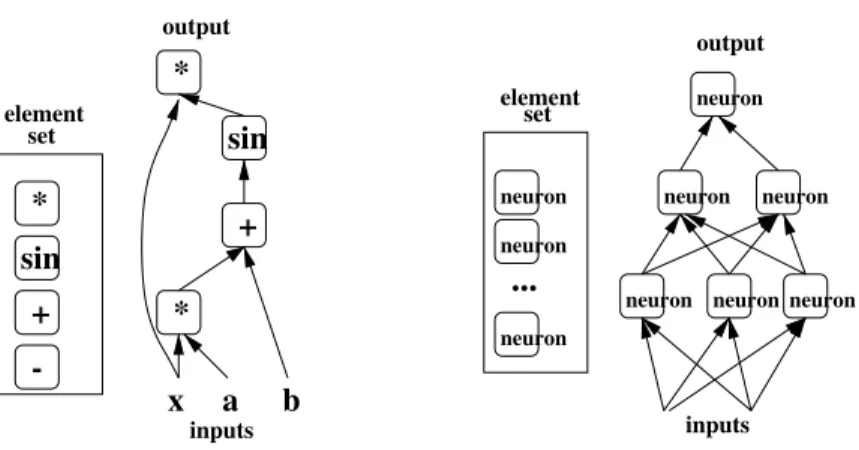
To formalize the notion of depth of architecture, one must introduce the notion of aset of computational elements. An example of such a set is the set of computations that can be performed logic gates. Another is the set of computations that can be performed by an artificial neuron (depending on the values of its synaptic weights). A function can be expressed by the composition of computational elements from a given set. It is defined by a graph which formalizes this composition, with one node per computational element. Depth of architecture refers to the depth of that graph, i.e., the longest path from an input node to an output node. When the set of computational elements is the set of computations an artificial neuron can perform, depth corresponds to the number of layers in a neural network. Let us explore the notion of depth with examples of architectures of diﬀerent depths. Consider the functionf(x) =x∗sin(a∗x+b). It can be expressed as the composi-tion of simple operacomposi-tions such as addicomposi-tion, subtraccomposi-tion, multiplicacomposi-tion,

(18)

15

x *

sin

+ *

sin +

neuron

neuron neuron neuron neuron neuron

neuron

set element

...

inputs output

*

b

-element set

output

inputsa

Fig. 2.1 Examples of functions represented by a graph of computations, where each node is taken in some “element set” of allowed computations. Left, the elements are{∗,+,−,sin}∪ R. The architecture computesx∗sin(a∗x+b) and has depth 4. Right, the elements are

artificial neurons computingf(x) = tanh(b+w′_x_{); each element in the set has a di}_ﬀ_erent

(w, b) parameter. The architecture is a multi-layer neural network of depth 3.

and the sin operation, as illustrated in Figure 2.1. In the example, there would be a diﬀerent node for the multiplication a_∗x and for the final multiplication byx. Each node in the graph is associated with an out-put value obtained by applying some function on inout-put values that are the outputs of other nodes of the graph. For example, in a logic circuit each node can compute a Boolean function taken from a small set of Boolean functions. The graph as a whole has input nodes and output nodes and computes a function from input to output. Thedepth of an architecture is the maximum length of a path from any input of the graph to any output of the graph, i.e., 4 in the case ofx∗sin(a∗x+b) in Figure 2.1.

• If we include aﬃne operations and their possible composition with sigmoids in the set of computational elements, linear regression and logistic regression have depth 1, i.e., have a single level.

(19)

K(x,xi) for each prototype xi (a selected representative

training example) and matches the input vector x with the prototypes xi. The second level performs an aﬃne

combina-tion b+!_iαiK(x,xi) to associate the matching prototypes

xi with the expected response.

• When we put artificial neurons (aﬃne transformation fol-lowed by a non-linearity) in our set of elements, we obtain ordinary multi-layer neural networks [156]. With the most common choice of one hidden layer, they also have depth two (the hidden layer and the output layer).

• Decision trees can also be seen as having two levels, as dis-cussed in Section 3.1.

• Boosting [52] usually adds one level to its base learners: that level computes a vote or linear combination of the outputs of the base learners.

• Stacking [205] is another meta-learning algorithm that adds one level.

• Based on current knowledge of brain anatomy [173], it appears that the cortex can be seen as a deep architecture, with 5–10 levels just for the visual system.

Although depth depends on the choice of the set of allowed com-putations for each element, graphs associated with one set can often be converted to graphs associated with another by an graph transfor-mation in a way that multiplies depth. Theoretical results suggest that it is not the absolute number of levels that matters, but the number of levels relative to how many are required to represent eﬃciently the target function (with some choice of set of computational elements).

2.1 Computational Complexity

(20)

2.1 Computational Complexity 17

A two-layer circuit of logic gates can represent any Boolean func-tion [127]. Any Boolean funcfunc-tion can be written as a sum of products (disjunctive normal form: AND gates on the first layer with optional negation of inputs, and OR gate on the second layer) or a product of sums (conjunctive normal form: OR gates on the first layer with optional negation of inputs, and AND gate on the second layer). To understand the limitations of shallow architectures, the first result to consider is that with depth-two logical circuits, most Boolean func-tions require an exponential (with respect to input size) number of logic gates [198] to be represented.

More interestingly, there are functions computable with a polynomial-size logic gates circuit of depthk that require exponential size when restricted to depth k−1 [62]. The proof of this theorem relies on earlier results [208] showing thatd-bit parity circuits of depth 2 have exponential size. The d-bit parity functionis defined as usual:

parity : (b1, . . . , bd)∈{0,1}d$→

⎧ ⎪ ⎨ ⎪ ⎩

1, if !d

i=1

biis even

0, otherwise.

One might wonder whether these computational complexity results for Boolean circuits are relevant to machine learning. See [140] for an early survey of theoretical results in computational complexity relevant to learning algorithms. Interestingly, many of the results for Boolean circuits can be generalized to architectures whose computational ele-ments arelinear thresholdunits (also known as artificial neurons [125]), which compute

(21)

Of particular interest is the following theorem, which applies to monotone weighted threshold circuits(i.e., multi-layer neural networks with linear threshold units and positive weights) when trying to repre-sent a function compactly reprerepre-sentable with a depthk circuit:

Theorem 2.1. A monotone weighted threshold circuit of depthk₋1 computing a functionfk∈Fk,N has size at least 2cN for some constant

c >0 andN > N0 [63].

The class of functionsFk,N is defined as follows. It contains functions

withN2k−2 inputs, defined by a depth k circuit that is a tree. At the leaves of the tree there are unnegated input variables, and the function value is at the root. The ith level from the bottom consists of AND gates wheniis even and OR gates wheniis odd. The fan-in at the top and bottom level isN and at all other levels it is N2.

The above results do not prove that other classes of functions (such as those we want to learn to perform AI tasks) require deep architec-tures, nor that these demonstrated limitations apply to other types of circuits. However, these theoretical results beg the question: are the depth 1, 2 and 3 architectures (typically found in most machine learn-ing algorithms) too shallow to represent eﬃciently more complicated functions of the kind needed for AI tasks? Results such as the above theorem also suggest thatthere might be no universally right depth: each function (i.e., each task) might require a particular minimum depth (for a given set of computational elements). We should therefore strive to develop learning algorithms that use the data to determine the depth of the final architecture. Note also that recursive computation defines a computation graph whose depth increases linearly with the number of iterations.

2.2 Informal Arguments

(22)

2.2 Informal Arguments 19

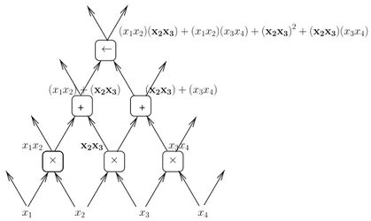
that a function ishighly varying when a piecewise approximation (e.g., piecewise-constant or piecewise-linear) of that function would require a large number of pieces. A deep architecture is a composition of many operations, and it could in any case be represented by a possibly very large depth-2 architecture. The composition of computational units in a small but deep circuit can actually be seen as an efficient “factorization” of a large but shallow circuit. Reorganizing the way in which compu-tational units are composed can have a drastic effect on the efficiency of representation size. For example, imagine a depth 2krepresentation of polynomials where odd layers implement products and even layers implement sums. This architecture can be seen as a particularly effi-cient factorization, which when expanded into a depth 2 architecture such as a sum of products, might require a huge number of terms in the sum: consider a level 1 product (likex2x3 in Figure 2.2) from the depth

2karchitecture. It could occur many times as a factor in many terms of the depth 2 architecture. One can see in this example that deep archi-tectures can be advantageous if some computations (e.g., at one level) can be shared (when considering the expanded depth 2 expression): in that case, the overall expression to be represented can be factored out, i.e., represented more compactly with a deep architecture.

Fig. 2.2 Example of polynomial circuit (with products on odd layers and sums on even ones) illustrating the factorization enjoyed by a deep architecture. For example the level-1 productx2x3would occur many times (exponential in depth) in a depth 2 (sum of product)

(23)

Further examples suggesting greater expressive power of deep archi-tectures and their potential for AI and machine learning are also dis-cussed by [19]. An earlier discussion of the expected advantages of deeper architectures in a more cognitive perspective is found in [191]. Note that connectionist cognitive psychologists have been studying for long time the idea of neural computation organized with a hierarchy of levels of representation corresponding to diﬀerent levels of abstrac-tion, with a distributed representation at each level [67, 68, 123, 122, 124, 157]. The modern deep architecture approaches discussed here owe a lot to these early developments. These concepts were introduced in cognitive psychology (and then in computer science / AI) in order to explain phenomena that were not as naturally captured by earlier cog-nitive models, and also to connect the cogcog-nitive explanation with the computational characteristics of the neural substrate.

(24)

3

Local vs Non-Local Generalization

3.1 The Limits of Matching Local Templates

How can a learning algorithm compactly represent a “complicated” function of the input, i.e., one that has many more variations than the number of available training examples? This question is both con-nected to the depth question and to the question of locality of estima-tors. We argue that local estimators are inappropriate to learn highly varying functions, even though they can potentially be represented eﬃ-ciently with deep architectures. An estimator that islocal in input space obtains good generalization for a new input x by mostly exploiting training examples in the neighborhood ofx. For example, the k near-est neighbors of the tnear-est pointx, among the training examples, vote for the prediction at x. Local estimators implicitly or explicitly partition the input space in regions (possibly in a soft rather than hard way) and require diﬀerent parameters or degrees of freedom to account for the possible shape of the target function in each of the regions. When many regions are necessary because the function is highly varying, the number of required parameters will also be large, and thus the number of examples needed to achieve good generalization.

(25)

22 Local vs Non-Local Generalization

The local generalization issue is directly connected to the literature on thecurse of dimensionality, but the results we cite show that what matters for generalization is not dimensionality, but instead the number of “variations” of the function we wish to obtain after learning. For example, if the function represented by the model is piecewise-constant (e.g., decision trees), then the question that matters is the number of pieces required to approximate properly the target function. There are connections between the number of variations and the input dimension: one can readily design families of target functions for which the number of variations is exponential in the input dimension, such as the parity function withdinputs.

Architectures based on matching local templates can be thought of as having two levels. The first level is made of a set of templates which can be matched to the input. A template unit will output a value that indicates the degree of matching. The second level combines these values, typically with a simple linear combination (an OR-like operation), in order to estimate the desired output. One can think of this linear combination as performing a kind of interpolation in order to produce an answer in the region of input space that is between the templates.

The prototypical example of architectures based on matching local templates is thekernel machine [166]

f(x) =b+&

i

αiK(x,xi), (3.1)

wherebandαi form the second level, while on the first level, thekernel

functionK(x,xi) matches the input xto the training examplexi (the

sum runs over some or all of the input patterns in the training set). In the above equation, f(x) could be for example, the discriminant function of a classifier, or the output of a regression predictor.

A kernel islocal when K(x,xi)>ρ is true only forx in some

con-nected region aroundxi (for some thresholdρ). The size of that region

can usually be controlled by a hyper-parameter of the kernel func-tion. An example of local kernel is the Gaussian kernel K(x,xi) =

e−||x−xi||2/σ2, where σ controls the size of the region around xi. We

(26)

3.1 The Limits of Matching Local Templates 23

it can be written as a product of one-dimensional conditions:K(u,v) =

'

je−(uj−vj)

2_/σ2

. If |uj −vj|/σ is small for all dimensionsj, then the

pattern matches and K(u,v) is large. If |uj −vj|/σ is large for a

singlej, then there is no match and K(u,v) is small.

Well-known examples of kernel machines include not only Support Vector Machines (SVMs) [24, 39] and Gaussian processes [203] 1 _for classification and regression, but also classical non-parametric learning algorithms for classification, regression and density estimation, such as thek-nearest neighbor algorithm, Nadaraya-Watson or Parzen windows density, regression estimators, etc. Below, we discussmanifold learning algorithmssuch as Isomap and LLE that can also be seen as local kernel machines, as well as related semi-supervised learning algorithms also based on the construction of aneighborhood graph (with one node per example and arcs between neighboring examples).

Kernel machines with a local kernel yield generalization by exploit-ing what could be called thesmoothness prior: the assumption that the target function is smooth or can be well approximated with a smooth function. For example, in supervised learning, if we have the train-ing example (xi, yi), then it makes sense to construct a predictorf(x)

which will output something close to yi when x is close to xi. Note

how this prior requires defining a notion of proximity in input space. This is a useful prior, but one of the claims made [13] and [19] is that such a prior is often insuﬃcient to generalize when the target function is highly varying in input space.

The limitations of a fixed generic kernel such as the Gaussian ker-nel have motivated a lot of research indesigning kernelsbased on prior knowledge about the task [38, 56, 89, 167]. However, if we lack suﬃ-cient prior knowledge for designing an appropriate kernel, can we learn it? This question also motivated much research [40, 96, 196], and deep architectures can be viewed as a promising development in this direc-tion. It has been shown that a Gaussian Process kernel machine can be improved using a Deep Belief Network to learn a feature space [160]: after training the Deep Belief Network, its parameters are used to

(27)

initialize a deterministic non-linear transformation (a multi-layer neu-ral network) that computes a feature vector (a new feature space for the data), and that transformation can be tuned to minimize the prediction error made by the Gaussian process, using a gradient-based optimiza-tion. The feature space can be seen as a learned representation of the data. Good representations bring close to each other examples which share abstract characteristics that are relevant factors of variation of the data distribution. Learning algorithms for deep architectures can be seen as ways to learn a good feature space for kernel machines.

Consider one direction v in which a target function f (what the learner should ideally capture) goes up and down (i.e., asα increases,

f(x+αv)₋bcrosses 0, becomes positive, then negative, positive, then negative, etc.), in a series of “bumps”. Following [165], [13, 19] show that for kernel machines with a Gaussian kernel, the required number of examples grows linearly with the number of bumps in the target function to be learned. They also show that for a maximally varying function such as the parity function, the number of examples necessary to achieve some error rate with a Gaussian kernel machine is expo-nential in the input dimension. For a learner that only relies on the prior that the target function is locally smooth (e.g., Gaussian kernel machines), learning a function with many sign changes in one direc-tion is fundamentally diﬃcult (requiring a large VC-dimension, and a correspondingly large number of examples). However, learning could work with other classes of functions in which the pattern of varia-tions is captured compactly (a trivial example is when the variavaria-tions are periodic and the class of functions includes periodic functions that approximately match).

(28)

3.1 The Limits of Matching Local Templates 25

Of course this could only happen if there were underlying regularities to be captured in the target function; we expect this property to hold in AI tasks.

Estimators that are local in input space are found not only in super-vised learning algorithms such as those discussed above, but also in unsupervised and semi-supervised learning algorithms, e.g., Locally Linear Embedding [155], Isomap [185], kernel Principal Component Analysis [168] (or kernel PCA) Laplacian Eigenmaps [10], Manifold Charting [26], spectral clustering algorithms [199], and kernel-based non-parametric semi-supervised algorithms [9, 44, 209, 210]. Most of these unsupervised and semi-supervised algorithms rely on the neigh-borhood graph: a graph with one node per example and arcs between near neighbors. With these algorithms, one can get a geometric intu-ition of what they are doing, as well as how being local estimators can hinder them. This is illustrated with the example in Figure 3.1 in the case of manifold learning. Here again, it was found that in order to

(29)

cover the many possible variations in the function to be learned, one needs a number of examples proportional to the number of variations to be covered [21].

Finally let us consider the case of semi-supervised learning rithms based on the neighborhood graph [9, 44, 209, 210]. These algo-rithms partition the neighborhood graph in regions of constant label. It can be shown that the number of regions with constant label cannot be greater than the number of labeled examples [13]. Hence one needs at least as many labeled examples as there are variations of interest for the classification. This can be prohibitive if the decision surface of interest has a very large number of variations.

Decision trees [28] are among the best studied learning algorithms. Because they can focus on specific subsets of input variables, at first blush they seem non-local. However, they are also local estimators in the sense of relying on a partition of the input space and using separate parameters for each region [14], with each region associated with a leaf of the decision tree. This means that they also suﬀer from the limita-tion discussed above for other non-parametric learning algorithms: they need at least as many training examples as there are variations of inter-est in the target function, and they cannot generalize to new variations not covered in the training set. Theoretical analysis [14] shows specific classes of functions for which the number of training examples neces-sary to achieve a given error rate is exponential in the input dimension. This analysis is built along lines similar to ideas exploited previously in the computational complexity literature [41]. These results are also in line with previous empirical results [143, 194] showing that the gen-eralization performance of decision trees degrades when the number of variations in the target function increases.

(30)

3.2 Learning Distributed Representations 27

Partition 1

C3=0

C1=1

C2=1 C3=0

C1=0

C2=0 C3=0

C1=0

C2=1 C3=0

C1=1

C2=1 C3=1

C1=1

C2=0 C3=1

C1=1

C2=1 C3=1

C1=0 Partition 3

Partition 2

C2=0

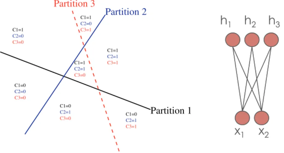
Fig. 3.2 Whereas a single decision tree (here just a two-way partition) can discriminate among a number of regions linear in the number of parameters (leaves), an ensemble of trees (left) can discriminate among a number of regions exponential in the number of trees, i.e., exponential in the total number of parameters (at least as long as the number of trees does not exceed the number of inputs, which is not quite the case here). Each distinguishable region is associated with one of the leaves of each tree (here there are three 2-way trees, each defining two regions, for a total of seven regions). This is equivalent to a multi-clustering, here three clusterings each associated with two regions. A binomial RBM with three hidden units (right) is a multi-clustering with 2 linearly separated regions per partition (each associated with one of the three binomial hidden units). A multi-clustering is therefore a distributed representation of the input pattern.

that tree. The identity of the leaf node in which the input pattern is associated for each tree forms a tuple that is a very rich description of the input pattern: it can represent a very large number of possible pat-terns, because the number of intersections of the leaf regions associated with thentrees can be exponential in n.

3.2 Learning Distributed Representations

(31)

the curse of dimensionality and the limitations of local generalization. A cartoonlocal representation for integers i_∈_{1,2, . . . , N_} is a vector r(i) of N bits with a single 1 and N ₋1 zeros, i.e., with jth element rj(i) =1i=j, called theone-hot representation of i. A distributed

rep-resentation for the same integer could be a vector of log₂N bits, which is a much more compact way to represent i. For the same number of possible configurations, a distributed representation can potentially be exponentially more compact than a very local one. Introducing the notion of sparsity (e.g., encouraging many units to take the value 0) allows for representations that are in between being fully local (i.e., maximally sparse) and non-sparse (i.e., dense) distributed representa-tions. Neurons in the cortex are believed to have a distributed and sparse representation [139], with around 1-4% of the neurons active at any one time [5, 113]. In practice, we often take advantage of represen-tations which are continuous-valued, which increases their expressive power. An example of continuous-valued local representation is one where the ith element varies according to some distance between the input and a prototype or region center, as with the Gaussian kernel dis-cussed in Section 3.1. In a distributed representation the input pattern is represented by a set of features that are not mutually exclusive, and might even be statistically independent. For example, clustering algo-rithms do not build a distributed representation since the clusters are essentially mutually exclusive, whereas Independent Component Anal-ysis (ICA) [11, 142] and Principal Component AnalAnal-ysis (PCA) [82] build a distributed representation.

Consider a discrete distributed representationr(x) for an input pat-ternx, whereri(x)∈{1, . . . M},i∈{1, . . . , N}. Eachri(x) can be seen

as a classification ofxintoM classes. As illustrated in Figure 3.2 (with M= 2), each ri(x) partitions thex-space inM regions, but the

(32)

3.2 Learning Distributed Representations 29

entries as the vocabulary size. On the other hand, a distributed repre-sentation could represent the word by concatenating in one vector indi-cators for syntactic features (e.g., distribution over parts of speech it can have), morphological features (which suﬃx or prefix does it have?), and semantic features (is it the name of a kind of animal? etc). Like in clustering, we construct discrete classes, but the potential number of combined classes is huge: we obtain what we call amulti-clusteringand that is similar to the idea of overlapping clusters and partial member-ships [65, 66] in the sense that cluster membermember-ships are not mutually exclusive. Whereas clustering forms a single partition and generally involves a heavy loss of information about the input, a multi-clustering provides a set of separate partitions of the input space. Identifying which region of each partition the input example belongs to forms a description of the input pattern which might be very rich, possibly not losing any information. The tuple of symbols specifying which region of each partition the input belongs to can be seen as a transformation of the input into a new space, where the statistical structure of the data and the factors of variation in it could be disentangled. This cor-responds to the kind of partition of x-space that an ensemble of trees can represent, as discussed in the previous section. This is also what we would like a deep architecture to capture, but with multiple levels of representation, the higher levels being more abstract and representing more complex regions of input space.

(33)

4

Neural Networks for Deep Architectures

4.1 Multi-Layer Neural Networks

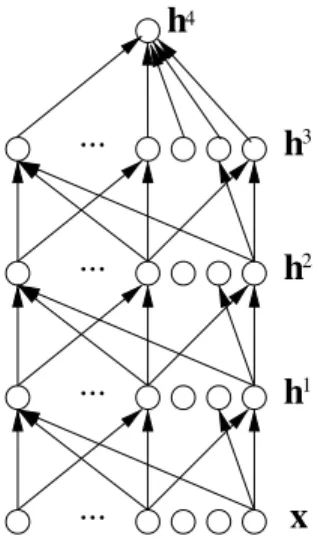
A typical set of equations for multi-layer neural networks [156] is the following. As illustrated in Figure 4.1, layer k computes an output vector hk _{using the output} _hk−1 _{of the previous layer, starting with} the input x=h0_,

hk_{= tanh(b}k ₊ _Wk_hk−1₎ _(4.1)

with parametersbk _{(a vector of oﬀsets) and}_Wk _{(a matrix of weights).}

The tanh is applied element-wise and can be replaced by sigm(u) = 1/(1 +e−u) = 1₂(tanh(u) + 1) or other saturating non-linearities. The top layer output hℓ _{is used for making a prediction and is combined}

with a supervised targetyinto a loss functionL(hℓ, y), typically convex inbℓ₊_Wℓ_hℓ−1_{. The output layer might have a non-linearity diﬀerent} from the one used in other layers, e.g., the softmax

hℓ i =

ebℓi+Wiℓhℓ−1 !

jeb ℓ

j+Wjℓhℓ−1

(4.2)

where W_iℓ is the ith row of Wℓ, hℓ_i is positive and !_ihℓ_i = 1. The softmax output hℓ

i can be used as estimator of P(Y =i|x), with the

(34)

4.2 The Challenge of Training Deep Neural Networks 31

...

x

h

...

h

4

3

2

1

Fig. 4.1 Multi-layer neural network, typically used in supervised learning to make a predic-tion or classificapredic-tion, through a series of layers, each of which combines an aﬃne operation and a non-linearity. Deterministic transformations are computed in a feedforward way from the inputx, through the hidden layershk_{, to the network output}_hℓ_{, which gets compared}

with a labelyto obtain the lossL(hℓ_{, y}_{) to be minimized.}

interpretation that Y is the class associated with input pattern x. In this case one often uses the negative conditional log-likelihood L(hℓ_{, y}_{) =}₋_log_P₍_Y ₌_y_|_{x) =}₋_log_hℓ

y as a loss, whose expected value

over (x, y) pairs is to be minimized.

4.2 The Challenge of Training Deep Neural Networks After having motivated the need for deep architectures that are non-local estimators, we now turn to the diﬃcult problem of training them. Experimental evidence suggests that training deep architectures is more diﬃcult than training shallow architectures [17, 50].

(35)

32 Neural Networks for Deep Architectures

Many unreported negative observations as well as the experimental results in [17, 50] suggest that gradient-based training of deep super-vised multi-layer neural networks (starting from random initialization) gets stuck in “apparent local minima or plateaus”,1 _{and that as the} architecture gets deeper, it becomes more diﬃcult to obtain good gen-eralization. When starting from random initialization, the solutions obtained with deeper neural networks appear to correspond to poor solutions that perform worse than the solutions obtained for networks with 1 or 2 hidden layers [17, 98]. This happens even though k+ 1-layer nets can easily represent what ak-layer net can represent (with-out much added capacity), whereas the converse is not true. However, it was discovered [73] that much better results could be achieved when pre-training each layer with an unsupervised learning algorithm, one layer after the other, starting with the first layer (that directly takes in input the observed x). The initial experiments used the RBM genera-tive model for each layer [73], and were followed by experiments yield-ing similar results usyield-ing variations of auto-encoders for trainyield-ing each layer [17, 153, 195]. Most of these papers exploit the idea of greedy layer-wise unsupervised learning (developed in more detail in the next section): first train the lower layer with an unsupervised learning algo-rithm (such as one for the RBM or some auto-encoder), giving rise to an initial set of parameter values for the first layer of a neural net-work. Then use the output of the first layer (a new representation for the raw input) as input for another layer, and similarly initialize that layer with an unsupervised learning algorithm. After having thus ini-tialized a number of layers, the whole neural network can be fine-tuned with respect to a supervised training criterion as usual. The advan-tage of unsupervised pre-training versus random initialization was clearly demonstrated in several statistical comparisons [17, 50, 98, 99]. What principles might explain the improvement in classification error observed in the literature when using unsupervised pre-training? One clue may help to identify the principles behind the success of some train-ing algorithms for deep architectures, and it comes from algorithms that

(36)

exploit neither RBMs nor auto-encoders [131, 202]. What these algo-rithms have in common with the training algoalgo-rithms based on RBMs and auto-encoders islayer-local unsupervised criteria, i.e., the idea that injecting anunsupervised training signal at each layermay help to guide the parameters of that layer towards better regions in parameter space. In [202], the neural networks are trained using pairs of examples (x,x),˜ which are either supposed to be “neighbors” (or of the same class) or not. Consider hk_{(x) the level-}_k _{representation of} _x _{in the model.}

A local training criterion is defined at each layer that pushes the inter-mediate representationshk_{(x) and}_hk_(˜_{x) either towards each other or}

away from each other, according to whetherxand ˜xare supposed to be neighbors or not (e.g., k-nearest neighbors in input space). The same criterion had already been used successfully to learn a low-dimensional embedding with an unsupervised manifold learning algorithm [59] but is here [202] applied at one or more intermediate layer of the neural net-work. Following the idea of slow feature analysis [23, 131, 204] exploit the temporal constancy of high-level abstraction to provide an unsu-pervised guide to intermediate layers: successive frames are likely to contain the same object.

Clearly, test errors can be significantly improved with these tech-niques, at least for the types of tasks studied, but why? One basic question to ask is whether the improvement is basically due to better optimization or to better regularization. As discussed below, the answer may not fit the usual definition of optimization and regularization.

(37)

ones that correspond to the unsupervised training, i.e., hopefully cor-responding to solutions capturing significant statistical structure in the input. On the other hand, other experiments [17, 98] suggest that poor tuning of the lower layers might be responsible for the worse results without pre-training: when the top hidden layer is constrained (forced to be small) thedeep networks with random initialization (no unsuper-vised pre-training) do poorly on both training and test sets, and much worse than pre-trained networks. In the experiments mentioned earlier where training error goes to zero, it was always the case that the num-ber of hidden units in each layer (a hyper-parameter) was allowed to be as large as necessary (to minimize error on a validation set). The explanatory hypothesis proposed in [17, 98] is that when the top hidden layer is unconstrained, the top two layers (corresponding to a regular 1-hidden-layer neural net) are sufficient to fit the training set, using as input the representation computed by the lower layers, even if that rep-resentation is poor. On the other hand, with unsupervised pre-training, the lower layers are ‘better optimized’, and a smaller top layer suffices to get a low training error but also yields better generalization. Other experiments described in [50] are also consistent with the explanation that with random parameter initialization, the lower layers (closer to the input layer) are poorly trained. These experiments show that the effect of unsupervised pre-training is most marked for the lower layers of a deep architecture.

We know from experience that a two-layer network (one hidden layer) can be well trained in general, and that from the point of view of the top two layers in a deep network, they form a shallow network whose input is the output of the lower layers. Optimizing the last layer of a deep neural network is a convex optimization problem for the training criteria commonly used. Optimizing the last two layers, although not convex, is known to be much easier than optimizing a deep network (in fact when the number of hidden units goes to infinity, the training criterion of a two-layer network can be cast as convex [18]).

(38)

generalization than shallow neural networks. When training error is low and test error is high, we usually call the phenomenon overfitting. Since unsupervised pre-training brings test error down, that would point to it as a kind of data-dependent regularizer. Other strong evidence has been presented suggesting that unsupervised pre-training acts like a regular-izer [50]: in particular, when there is not enough capacity, unsupervised pre-training tends to hurt generalization, and when the training set size is “small” (e.g., MNIST, with less than hundred thousand examples), although unsupervised pre-training brings improved test error, it tends to produce larger training error.

On the other hand, for much larger training sets, with better initial-ization of the lower hidden layers, both training and generalinitial-ization error can be made significantly lower when using unsupervised pre-training (see Figure 4.2 and discussion below). We hypothesize that in a well-trained deep neural network, the hidden layers form a “good” repre-sentation of the data, which helps to make good predictions. When the lower layers are poorly initialized, these deterministic and continuous representations generally keep most of the information about the input, but these representations might scramble the input and hurt rather than help the top layers to perform classifications that generalize well. According to this hypothesis, although replacing the top two layers of a deep neural network by convex machinery such as a Gaussian process or an SVM can yield some improvements [19], especially on the training error, it would not help much in terms of generalization if the lower layers have not been suﬃciently optimized, i.e., if a good representation of the raw input has not been discovered.

(39)

0 1 2 3 4 5 6 7 8 9 10

x 106 10−4

10−3 10−2 10−1 100 101

Number of examples seen

Online classification error

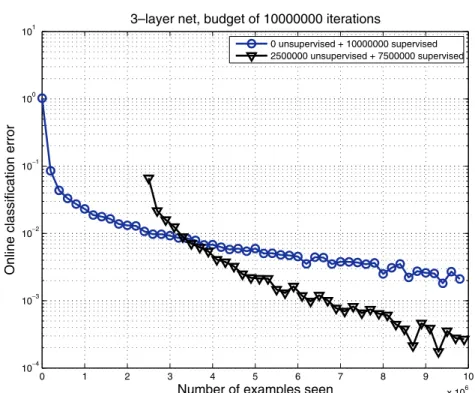
3–layer net, budget of 10000000 iterations

0 unsupervised + 10000000 supervised 2500000 unsupervised + 7500000 supervised

Fig. 4.2 Deep architecture trained online with 10 million examples of digit images, either with pre-training (triangles) or without (circles). The classification error shown (vertical axis, log-scale) is computed online on the next 1000 examples, plotted against the number of examples seen from the beginning. The first 2.5 million examples are used for unsuper-vised pre-training (of a stack of denoising auto-encoders). The oscillations near the end are because the error rate is too close to 0, making the sampling variations appear large on the log-scale. Whereas with a very large training set regularization eﬀects should dissipate, one can see that without pre-training, training converges to a poorer apparent local minimum: unsupervised pre-training helps to find a better minimum of the online error. Experiments were performed by Dumitru Erhan.

(40)

involved in estimatingP(X) andP(Y_|X),4then each (X, Y) pair brings information on P(Y|X) not only in the usual way but also through P(X). For example, in a Deep Belief Net, both distributions share essentially the same parameters, so the parameters involved in esti-matingP(Y_|X) benefit from a form of data-dependent regularization: they have to agree to some extent withP(Y|X) as well as with P(X). Let us return to the optimization versus regularization explanation of the better results obtained with unsupervised pre-training. Note how one should be careful when using the word ’optimization’ here. We do not have an optimization difficulty in the usual sense of the word. Indeed, from the point of view of the whole network, there is no dif-ficulty since one can drive training error very low, by relying mostly on the top two layers. However, if one considers the problem of tun-ing the lower layers (while keeptun-ing small either the number of hidden units of the penultimate layer (i.e., top hidden layer) or the magnitude of the weights of the top two layers), then one can maybe talk about an optimization difficulty. One way to reconcile the optimization and regularization viewpoints might be to consider the truly online setting (where examples come from an infinite stream and one does not cycle back through a training set). In that case, online gradient descent is performing a stochastic optimization of the generalization error. If the effect of unsupervised pre-training was purely one of regularization, one would expect that with a virtually infinite training set, online error with or without pre-training would converge to the same level. On the other hand, if the explanatory hypothesis presented here is correct, we would expect that unsupervised pre-training would bring clear benefits even in the online setting. To explore that question, we have used the ‘infinite MNIST’ dataset [120], i.e., a virtually infinite stream of MNIST-like digit images (obtained by random translations, rotations, scaling, etc. defined in [176]). As illustrated in Figure 4.2, a 3-hidden layer neural network trained online converges to significantly lower error when it is pre-trained (as a Stacked Denoising Auto-Encoder, see Section 7.2). The figure shows progress with the online error (on the next 1000

(41)

examples), an unbiased Monte-Carlo estimate of generalization error. The first 2.5 million updates are used for unsupervised pre-training. The figure strongly suggests that unsupervised pre-training converges to a lower error, i.e., that it acts not only as a regularizer but also to find better minima of the optimized criterion. In spite of appearances, this does not contradict the regularization hypothesis: because of local minima, the regularization eﬀect persists even as the number of exam-ples goes to infinity. The flip side of this interpretation is that once the dynamics are trapped near some apparent local minimum, more labeled examples do not provide a lot more new information.

(42)

4.3 Unsupervised Learning for Deep Architectures 39

4.3 Unsupervised Learning for Deep Architectures

As we have seen above, layer-wise unsupervised learning has been a crucial component of all the successful learning algorithms for deep architectures up to now. If gradients of a criterion defined at the out-put layer become less useful as they are propagated backwards to lower layers, it is reasonable to believe that an unsupervised learning criterion defined at the level of a single layer could be used to move its param-eters in a favorable direction. It would be reasonable to expect this if the single-layer learning algorithm discovered a representation that cap-tures statistical regularities of the layer’s input. PCA and the standard variants of ICA requiring as many causes as signals seem inappropriate because they generally do not make sense in the so-called overcom-plete case, where the number of outputs of the layer is greater than the number of its inputs. This suggests looking in the direction of exten-sions of ICA to deal with the overcomplete case [78, 87, 115, 184], as well as algorithms related to PCA and ICA, such as auto-encoders and RBMs, which can be applied in the overcomplete case. Indeed, experi-ments performed with these one-layer unsupervised learning algorithms in the context of a multi-layer system confirm this idea [17, 73, 153]. Furthermore, stacking linear projections (e.g., two layers of PCA) is still a linear transformation, i.e., not building deeper architectures.

(43)

the features learned with the first layer could extract slightly higher-level features. In this way, one could imagine that higher-higher-level abstrac-tions that characterize the input could emerge. Note how in this process all learning could remain local to each layer, therefore side-stepping the issue of gradient diﬀusion that might be hurting gradient-based learn-ing of deep neural networks, when we try to optimize a slearn-ingle global criterion. This motivates the next section, where we discuss deep gen-erative architectures and introduce Deep Belief Networks formally.

4.4 Deep Generative Architectures

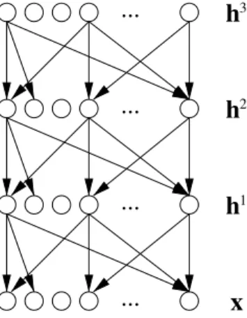
Besides being useful for pre-training a supervised predictor, unsuper-vised learning in deep architectures can be of interest to learn a distri-bution and generate samples from it. Generative models can often be represented as graphical models [91]: these are visualized as graphs in which nodes represent random variables and arcs say something about the type of dependency existing between the random variables. The joint distribution of all the variables can be written in terms of prod-ucts involving only a node and its neighbors in the graph. With directed arcs (defining parenthood), a node is conditionally independent of its ancestors, given its parents. Some of the random variables in a graphi-cal model can be observed, and others cannot (graphi-called hidden variables). Sigmoid belief networks are generative multi-layer neural networks that were proposed and studied before 2006, and trained using variational approximations [42, 72, 164, 189]. In a sigmoid belief network, the units (typically binary random variables) in each layer are independent given the values of the units in the layer above, as illustrated in Figure 4.3. The typical parametrization of these conditional distributions (going downwards instead of upwards in ordinary neural nets) is similar to the neuron activation equation of Equation (4.1):

P(hk_i = 1_|hk+1) = sigm(bk_i +&

j

W_i,jk+1hk_j+1) (4.3) where hk

i is the binary activation of hidden node i in layer k, hk is

the vector (hk

(44)

4.4 Deep Generative Architectures 41

2

...

_x

h

1 3

Fig. 4.3 Example of a generative multi-layer neural network, here a sigmoid belief network, represented as a directed graphical model (with one node per random variable, and directed arcs indicating direct dependence). The observed data isxand the hidden factors at level

kare the elements of vectorhk_{. The top layer}_h3_{has a factorized prior.}

empirical distribution of the training set, or the generating distribution for our training examples). The bottom layer generates a vector x in the input space, and we would like the model to give high probability to the training data. Considering multiple levels, the generative model is thus decomposed as follows:

P(x,h1, . . . ,hℓ) =P(hℓ)

(_ℓ₋₁ )

k=1

P(hk_|hk+1)

*

P(x_|h1) (4.4)

and marginalization yields P(x), but this is intractable in practice except for tiny models. In a sigmoid belief network, the top level prior P(hℓ) is generally chosen to be factorized, i.e., very simple: P(hℓ) ='_iP(hℓ_i), and a single Bernoulli parameter is required for each P(hℓ_i = 1) in the case of binary units.

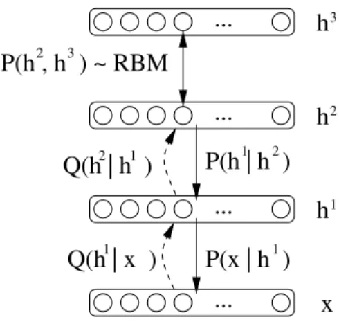
Deep Belief Networks are similar to sigmoid belief networks, but with a slightly diﬀerent parametrization for the top two layers, as illus-trated in Figure 4.4:

P(x,h1, . . . ,hℓ) =P(hℓ−1,hℓ)

(_ℓ₋₂ )

k=1

P(hk_|hk+1)

*

(45)

...

x

h

1 3

...

_h

h

2 2 3

h h

P( , ) ~ RBM

Fig. 4.4 Graphical model of a Deep Belief Network with observed vector xand hidden layers h1_,_h2 _and_h3_{. Notation is as in Figure 4.3. The structure is similar to a sigmoid} belief network, except for the top two layers. Instead of having a factorized prior forP(h3_), the joint of the top two layers,P(h2_,_h3_{), is a Restricted Boltzmann Machine. The model} is mixed, with double arrows on the arcs between the top two layers because an RBM is an undirected graphical model rather than a directed one.

h

...

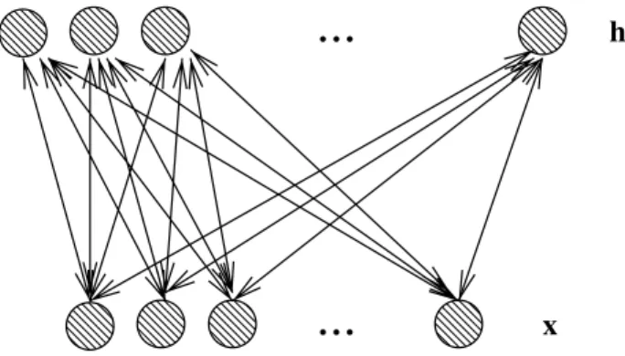
x

Fig. 4.5 Undirected graphical model of a Restricted Boltzmann Machine (RBM). There are no links between units of the same layer, only between input (or visible) unitsxjand

hidden unitshi, making the conditionalsP(h|x) andP(x|h) factorize conveniently.

The joint distribution of the top two layers is a Restricted Boltzmann Machine (RBM),

(46)

4.5 Convolutional Neural Networks 43

with a diﬀerent learning algorithm, which exploits the notion of train-ing greedily one layer at a time, buildtrain-ing up gradually more abstract representations of the raw input into the posteriorsP(hk_|_{x). A detailed}

description of RBMs and of the greedy layer-wise training algorithms for deep architectures follows in Sections 5 and 6.

4.5 Convolutional Neural Networks

Although deep supervised neural networks were generally found too diﬃcult to train before the use of unsupervised pre-training, there is one notable exception: convolutional neural networks. Convolutional nets were inspired by the visual system’s structure, and in particular by the models of it proposed by [83]. The first computational models based on these local connectivities between neurons and on hierarchi-cally organized transformations of the image are found in Fukushima’s Neocognitron [54]. As he recognized, when neurons with the same parameters are applied on patches of the previous layer at diﬀerent locations, a form of translational invariance is obtained. Later, LeCun and collaborators, following up on this idea, designed and trained con-volutional networks using the error gradient, obtaining state-of-the-art performance [101, 104] on several pattern recognition tasks. Modern understanding of the physiology of the visual system is consistent with the processing style found in convolutional networks [173], at least for the quick recognition of objects, i.e., without the benefit of attention and top-down feedback connections. To this day, pattern recognition systems based on convolutional neural networks are among the best per-forming systems. This has been shown clearly for handwritten character recognition [101], which has served as a machine learning benchmark for many years.5

Concerning our discussion of training deep architectures, the exam-ple of convolutional neural networks [101, 104, 153, 175] is interesting because they typically have five, six or seven layers, a number of lay-ers which makes fully connected neural networks almost impossible to train properly when initialized randomly. What is particular in their

(47)

architecture that might explain their good generalization performance in vision tasks?

LeCun’s convolutional neural networks are organized in layers of two types: convolutional layers and subsampling layers. Each layer has atopographic structure, i.e., each neuron is associated with a fixed two-dimensional position that corresponds to a location in the input image, along with a receptive field (the region of the input image that influ-ences the response of the neuron). At each location of each layer, there are a number of different neurons, each with its set of input weights, associated with neurons in a rectangular patch in the previous layer. The same set of weights, but a different input rectangular patch, are associated with neurons at different locations.

One untested hypothesis is that the small fan-in of these neurons (few inputs per neuron) helps gradients to propagate through so many layers without diffusing so much as to become useless. Note that this alone would not suffice to explain the success of convolutional net-works, since random sparse connectivity is not enough to yield good results in deep neural networks. However, an effect of the fan-in would be consistent with the idea that gradients propagated through many paths gradually become too diffuse, i.e., the credit or blame for the output error is distributed too widely and thinly. Another hypothesis (which does not necessarily exclude the first) is that the hierarchical local connectivity structure is a very strong prior that is particularly appropriate for vision tasks, and sets the parameters of the whole net-work in a favorable region (with all non-connections corresponding to zero weight) from which gradient-based optimization works well. The fact is that even withrandom weightsin the first layers, a convolutional neural network performs well [151], i.e., better than a trained fully con-nected neural network but worse than a fully optimized convolutional neural network.