SQL-on-Hadoop: Full Circle Back to Shared-Nothing Database Architectures

(1)

SQL-on-Hadoop: Full Circle Back to Shared-Nothing

Database Architectures

Avrilia Floratou

IBM Almaden Research Center

Umar Farooq Minhas

Fatma ¨

Ozcan

ABSTRACT

SQL query processing for analytics over Hadoop data has recently gained significant traction. Among many systems providing some SQL support over Hadoop, Hive is the first native Hadoop system that uses an underlying framework such as MapReduce or Tez to process SQL-like statements. Impala, on the other hand, represents the new emerging class of SQL-on-Hadoop systems that exploit a shared-nothing parallel database architecture over Hadoop. Both systems optimize their data ingestion via columnar storage, and promote different file formats: ORC and Parquet. In this paper, we compare the performance of these two systems by conducting a set of cluster experiments using a TPC-H like benchmark and two TPC-DS inspired workloads. We also closely study the I/O effi-ciency of their columnar formats using a set of micro-benchmarks. Our results show that Impala is3.3Xto4.4Xfaster than Hive on MapReduce and2.1X to2.8X than Hive on Tez for the overall TPC-H experiments. Impala is also8.2Xto10Xfaster than Hive on MapReduce and about4.3X faster than Hive on Tez for the TPC-DS inspired experiments. Through detailed analysis of exper-imental results, we identify the reasons for this performance gap and examine the strengths and limitations of each system.

1. INTRODUCTION

Enterprises are using Hadoop as a central data repository for all their data coming from various sources, including operational sys-tems, social media and the web, sensors and smart devices, as well as their applications. Various Hadoop frameworks are used to man-age and run deep analytics in order to gain actionable insights from the data, including text analytics on unstructured text, log analysis over semi-structured data, as well as relational-like SQL processing over semi-structured and structured data.

SQL processing in particular has gained significant traction, as many enterprise data management tools rely on SQL, and many enterprise users are familiar and comfortable with it. As a re-sult, the number of SQL-on-Hadoop systems have increased signif-icantly. We can classify these systems into two general categories: Native Hadoop-based systems, and database-Hadoop hybrids. In the first category, Hive [6, 21] is the first SQL-like system over

This work is licensed under the Creative Commons Attribution-NonCommercial-NoDerivs 3.0 Unported License. To view a copy of this li-cense, visit http://creativecommons.org/licenses/by-nc-nd/3.0/. Obtain per-mission prior to any use beyond those covered by the license. Contact copyright holder by emailing [email protected]. Articles from this volume were invited to present their results at the 40th International Conference on Very Large Data Bases, September 1st - 5th 2014, Hangzhou, China. Proceedings of the VLDB Endowment, Vol. 7, No. 12

Hadoop, which uses another framework such as MapReduce or Tez to process SQL-like queries, leveraging its task scheduling and load balancing features. Shark [7, 24] is somewhat similar to Hive in that it uses another framework, Spark [8] as its runtime. In this category, Impala [10] moved away from MapReduce to a shared-nothing parallel database architecture. Impala runs queries using its own long-running daemons running on every HDFS DataNode, and instead of materializing intermediate results, pipelines them be-tween computation stages. Similar to Impala, LinkedIn Tajo [20], Facebook Presto [17], and MapR Drill [4], also resemble parallel databases and use long-running custom-built processes to execute SQL queries in a distributed fashion.

In the second category, Hadapt [2] also exploits Hadoop schedul-ing and fault-tolerance, but uses a relational database (PostgreSQL) to execute query fragments. Microsoft PolyBase [11] and Pivotal HAWQ [9], on the other hand, use database query optimization and planning to schedule query fragments, and directly read HDFS data into database workers for processing. Overall, we observe a big convergence to shared-nothing database architectures among the SQL-on-Hadoop systems.

In this paper, we focus on the first category of native SQL-on-Hadoop systems, and investigate the performance of Hive and Im-pala, highlighting their different design trade-offs through detailed experiments and analysis. We picked these two systems due to their popularity as well as their architectural differences. Impala and Hive are the SQL offerings from two major Hadoop distribution vendors, Cloudera and Hortonworks. As a result, they are widely used in the enterprise. There are other SQL-on-Hadoop systems, such as Presto and Tajo, but these systems are mainly used by com-panies that created them, and are not as widely used. Impala is a good representative of emerging SQL-on-Hadoop systems, such as Presto, and Tajo, which follow a shared-nothing database like ar-chitecture with custom-built daemons and custom data communi-cation protocols. Hive, on the other hand, represents another archi-tectural design where a run-time framework, such as MapReduce or Tez, is used for scheduling, data movement, and parallelization. Hive and Impala are used for analytical queries. Columnar data organization has been shown to improve the performance of such queries in the context of relational databases [1, 18]. As a result, columnar storage organization is also utilized for analytical queries over Hadoop data. RCFile [14] and Trevni [23] are early columnar file formats for HDFS data. While relational databases store each column data in a separate file, in Hadoop and HDFS, all columns are packed into a single file, similar to the PAX [3] data layout. Floratou et.al. [12] pointed out to several performance problems in RCFile. To address these shortcomings, Hortonworks and Mi-crosoft propose the ORC file format, which is the next generation of RCFile. Impala, on the other hand, is promoting the Parquet

(2)

file format, which is a columnar format inspired by Dremel’s [16] storage format. These two formats compete to become the defacto standard for Hadoop data storage for analytical queries.

In this paper, we delve into the details of these two storage for-mats to gain insights into their I/O characteristics. We conduct a de-tailed analysis of Impala and Hive using TPC-H data, stored as text, Parquet and ORC file formats. We also conduct experiments using a TPC-DS inspired workload. We also investigate the columnar storage formats in conjunction with the system promoting them.

Our experimental results show that:

• Impala’s database-like architecture provides significant perfor-mance gains, compared to Hive’s MapReduce or Tez based run-time. Hive on MapReduce is also impacted by the startup and scheduling overheads of the MapReduce framework, and pays the cost of writing intermediate results into HDFS. Impala, on the other hand, streams the data between stages of the query computation, resulting in significant performance improvements. But, Impala cannot recover from mid-query failures yet, as it needs to re-run the whole query in case of a failure. Hive on Tez eliminates the startup and materialization overheads of MapReduce, improving Hive’s overall performance. However, it does not avoid the Java deserialization overheads during scan operations and thus it is still slower than Impala.

• While Impala’s I/O subsystem provides much faster ingestion rates, the single threaded execution of joins and aggregations im-pedes the performance of complex queries.

• The Parquet format skips data more efficiently than the ORC file which tends to prefetch unnecessary data especially when a table contains a large number of columns. However, the built-in index in ORC file mitigates that problem when the data is sorted.

Our results reaffirm the clear advantages of a shared-nothing database architecture for analytical SQL queries over a MapReduce-based runtime. It is interesting to see the community to come full circle back to parallel database architectures, after the extensive comparisons and discussions [19, 13].

The rest of the paper is organized as follows: in Section 2, we first review the Hive and Impala architectures, as well as the ORC and the Parquet file formats. In Section 3, we present our anal-ysis on the cluster experiments. We investigate the I/O rates and effect of the ORC file’s index using a set of micro-benchmarks in Section 4, and conclude in Section 5.

2. BACKGROUND

2.1 Apache Hive

Hive [6] is the first SQL-on-Hadoop system built on top of Apache Hadoop [5] and thus exploits all the advantages of Hadoop includ-ing: its ability to scale out to thousands or tens of thousands of nodes, fault tolerance and high availability.

Hive implements a SQL-like query language namely HiveQL. HiveQL statements submitted to Hive are parsed, compiled, and optimized to produce a physical query execution plan. The plan is a Directed Acyclic Graph (DAG) of MapReduce tasks which is executed through the MapReduce framework or through the Tez framework in the latest Hive version. A HiveQL query is executed in a single Tez job when the Tez framework is used and is typically split into multiple MapReduce jobs when the MapReduce frame-work is used. Tez pipelines data through execution stages instead of creating temporary intermediate files. Thus, Tez avoids the startup, scheduling and materialization overheads of MapReduce.

The choice of join method and the order of joins significantly im-pact the performance of analytical queries. Hive supports two types

of join methods. The most generic form of join is called a

repar-titioned join, in which multiple map tasks read the input tables,

emitting the join (key, value) pair, where the key is the join column. These pairs are shuffled and distributed (over-the-network) to the reduce tasks, which perform the actual join operation. A second, more optimized, form of join supported by Hive is called map-side

join. Its main goal is to eliminate the shuffle and reduce phases of

the repartitioned join. Map-side join is applicable when one of the table is small. All the map tasks read the small table and perform the join processing in a map only job. Hive also supports predicate pushdown and partition elimination.

2.2 Cloudera Impala

Cloudera Impala [10] is another open-source project that imple-ments SQL processing capabilities over Hadoop data, and has been inspired by Google’s Dremel [16]. Impala supports a SQL-like query language which is a subset of SQL as well.

As opposed to Hive, instead of relying on another framework, Impala provides its own long running daemons on each node of the cluster and has a shared-nothing parallel database architecture. The main daemon process impaladcomprises the query planner, query coordinator, and the query execution engine. Impala supports two types of join algorithms: partitioned and broadcast, which are similar to Hive’s repartitioned join and map-side join, respectively. Impala compiles all queries into a pipelined execution plan.

Impala has a highly efficient I/O layer to read data stored in HDFS which spawns one I/O thread per disk on each node. The Impala I/O layer decouples the requests to read data (which is asyn-chronous), and the actual reading of the data (which is synasyn-chronous), keeping disks and CPUs highly utilized at all times. Impala also exploits the Streaming SIMD Extension (SSE) instructions, avail-able on the latest generation of Intel processors to parse and process textual data efficiently.

Impala still requires the working set of a query to fit in the ag-gregate physical memory of the cluster it runs on. This is a major limitation, which imposes strict constraints on the kind of datasets one is able to process with Impala.

2.3 Columnar File Formats

Columnar data organizations reduce disk I/O, and enable better compression and encoding schemes that significantly benefit an-alytical queries [18, 1]. Both Hive and Impala have implemented their own columnar storage formats, namely Hive’s Optimized Row Columnar (ORC) format and Impala’s Parquet columnar format.

2.3.1 Optimized Row Columnar (ORC) File Format

This file format is an optimized version of the previously pub-lished Row Columnar (RC) file format [14]. The ORC file for-mat provides storage efficiency by providing data encoding and block-level compression as well as better I/O efficiency through a lightweight built-in index that allows skipping row groups that do not pass a filtering predicate. The ORC file packs columns of a table in a PAX [3] like organization within an HDFS block. More specifically, an ORC file stores multiple groups of row data asstripes. Each ORC file has afile footerthat contains a list of stripes in the file, the number of rows stored in each stripe, the data type of each column, and column-level aggregates such ascount,sum,min, andmax. The stripe size is a configurable parameter and is typically set to256MB. Hive automatically sets the HDFS block size tomin(2∗stripe size,1.5GB), in order to ensure that the I/O requests operate on large chunks of local data.

Internally, each stripe is divided intoindex data,row data, and stripe footer, in that order. The data in each column

(3)

consists of multiple streams. For example, integer columns consist of two streams: the present bit stream which denotes whether the value is null and the actual data stream. The stripe footer contains a directory of the stream locations of each column. As part of the index data,minandmaxvalues for each column are stored, as well as the row positions within each column. Using the built-in index, row groups (default of10,000rows) can be skipped if the query predicate does not fall within the minimum and maximum values of the row group.

2.3.2 Parquet File Format

The Parquet columnar format has been designed to exploit ef-ficient compression and encoding schemes and to support nested data. It stores data grouped together in logical horizontal parti-tions calledrow groups. Every row group contains acolumn chunkfor each column in the table. A column chunk consists of multiplepagesand is guaranteed to be stored contiguously on disk. Parquet’s compression and encoding schemes work at a page level. Metadata is stored at all the levels in the hierarchy i.e., file, column chunk, and page. The Parquet readers first parse the meta-data to filter out the column chunks that must be accessed for a particular query and then read each column chunk sequentially.

Impala heavily makes use of the Parquet storage format but does not support nested columns yet. In Impala, all the data for each row group are kept in a separate Parquet data file stored on HDFS, to make sure that all the columns of a given row are stored on the same node. Impala automatically sets the HDFS block size and the Parquet file size to a maximum of1GB. In this way, I/O and network requests apply to a large chunk of data.

3. CLUSTER EXPERIMENTS

In this section, we explore the performance of Hive and Impala using a TPC-H like workload and two TPC-DS inspired workloads.

3.1 Hardware Configuration

For the experiments presented in this section, we use a 21 node cluster. One of the nodes hosts the HDFS NameNode and sec-ondary namenode, the Impala StateStore, and Catalog processes and the Hive Metastore (“control” node). The remaining 20 nodes are designated as “compute” nodes. Every node in the cluster has 2x Intel Xeon CPUs @ 2.20GHz, with 6x physical cores each (12 physical cores total), 11x SATA disks (2TB, 7k RPM), 1x 10 Giga-bit Ethernet card, and 96GB of RAM. Out of the 11 SATA disks, we use one for the operating system, while the remaining 10 disks are used for HDFS. Each node runs 64-bit Ubuntu Linux 12.04.

3.2 Software Configuration

For our experiments, we use Hive version 0.12 (Hive-MR) and Impala version 1.2.2 on top of Hadoop 2.0.0-cdh4.5.0. We also use Hive version 0.13 (Hive-Tez) on top of Tez 0.3.0 and Apache Hadoop 2.3.0.1 We configured Hadoop to run 12 containers per node (1 per core). The HDFS replication factor is set to 3 and the maximum JVM heap size is set to 7.5 GB per task. We config-ured Impala to use MySQL as the metastore. We run one impalad process on each compute node and assign 90 GB of memory to it. We enable short-circuit reads and block location tracking as per the Impala instructions. Short-circuit reads allow reading local data di-rectly from the filesystem. For this reason, this parameter is also enabled for the Hive experiments. Runtime code generation in Im-pala is enabled in all the experiments.

1_{In the following sections, when the term Hive is used, this applies} to both Hive-MR and Hive-Tez.

3.3 TPC-H like Workload

For our experiments, we use a TPC-H2 like workload, which has been used by both the Hive and Impala engineers to evaluate their systems. The workload scripts for Hive and Impala have been published by the developers of these systems3,4.

The workload contains the 22 read-only TPC-H queries but not the refresh streams. We use a TPC-H database with a scale factor of 1000 GB. We were not able to scale to larger TPC-H datasets because of Impala’s limitation to require the workload’s working set to fit in the cluster’s aggregate memory. However, as we will show in our analysis, this dataset can provide significant insights into the strengths and limitations of each system.

Although the workload scripts for both Hive and Impala are avail-able online, these do not take into account some of the new features of these systems. Hive has now support for nested sub-queries. In order to exploit this feature, we re-wrote 11 TPC-H queries. The remaining queries could not be further optimized since they already consist of a single query. Impala was able to execute these re-written queries and produce correct results, except for Query 18, which produced incorrect results when nested and had to be split into two queries.

In Hive-MR, we enabled various optimizations including: a) op-timization of correlated queries, b) predicate push-down and in-dex filtering when using the ORC file format, and c) map-side join and aggregation. When a query is split into multiple sub-queries, the intermediate results between sub-queries were materialized into temporary tables in HDFS using the same file format/compression codec with the base tables. Hive, when used out of the box, typ-ically generates a large number of reduce tasks that tend to neg-atively affect performance. We experimented with various num-bers of reduce tasks for the workload and found that in our envi-ronment 120 reducers produce the best performance since all the reduce tasks can complete in one reduce round. In Hive-Tez, we additionally enabled the vectorized execution engine.

For Impala, we computed table and column statistics for each table using theCOMPUTE STATSstatement. These statistics are used to optimize the join order and choose the join methods.

3.4 Data Preparation and Load Times

In this section, we describe the loading process in Hive and Im-pala. We used the ORC file format in Hive and the Parquet file format in Impala which are the popular columnar formats that each system advertises. We also experimented with the text file format (TXT) in order to examine the performance of each system when the data arrives in native uncompressed text format and needs to be processed right away. We experimented with all the compres-sion algorithms that are available for each columnar layout, namely

snappy and zlib for the ORC file format and snappy and gzip for the

Parquet format. Our results show that snappy compression provides slightly better query performance than zlib and gzip, for the TPC-H workload, on both file formats. For this reason, we only report results with snappy compression in both Hive and Impala.

We generated the data files using the TPC-H generator at 1TB scale factor and copied them into HDFS as plain text. We use a Hive query to convert the data from the text format to the ORC format. Similarly, we used an Impala query to load the data into the Parquet tables.

Table 2 presents the time to load all the TPC-H tables in each system, for each format that we used. It also shows the

aggre-2 http://www.tpc.org/tpch/ 3 https: //issues.apache.org/jira/browse/HIVE-600 4 https://github.com/kj-ki/tpc-h-impala

(4)

0 1 2 3 4 5 TXT ORC/Parquet ORC/Parquet(Snappy)

Normalized Arithmetic Mean

File Format (Compression Type) 5.0X 3.5X 3.3X 3.1X 2.3X 2.1X 1.1X _1.0X _1.0X Hive−MR Hive−Tez Impala 0 1 2 3 4 5 6 7 8 9 TXT ORC/Parquet ORC/Parquet(Snappy)

Normalized Geometric Mean

File Format (Compression Type) 8.2X 5.6X 5.1X 4.3X 3.4X _3.2X 1.3X _1.0X _1.0X Hive−MR Hive−Tez Impala

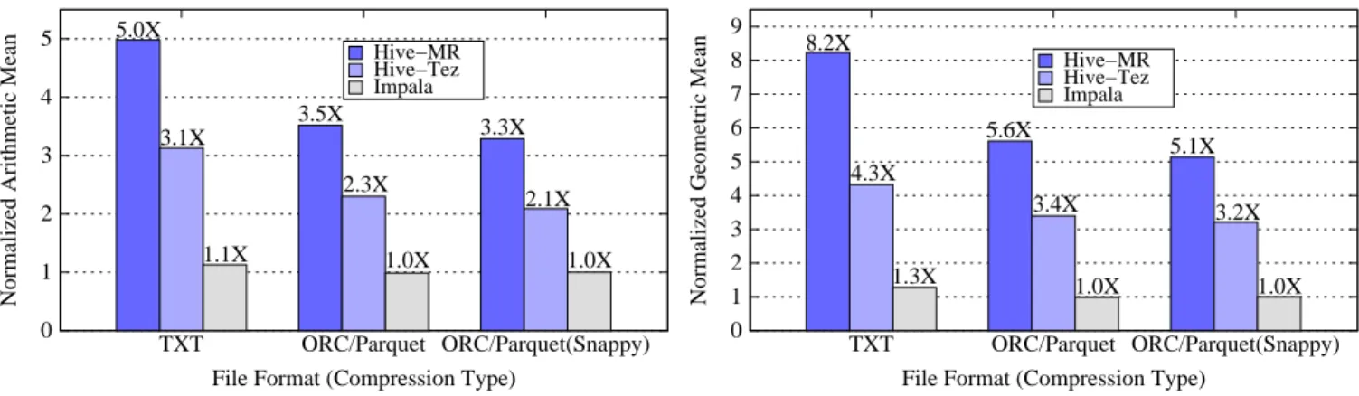
Figure 1: Hive-Impala Overall Comparison (Arithmetic Mean) Figure 2: Hive-Impala Overall Comparison (Geometric Mean)

Table 2: Data Loading in Hive and Impala System File Format Time Size (secs) (GB) Hive-MR ORC 3099 803 ORC-Snappy 5191 337 Hive-Tez ORC 1583 629 ORC-Snappy 1606 290 Impala Parquet 784 623 Parquet-Snappy 822 316

gate size of the tables.5 In this table and in the following sections, we will use term ORC or Parquet to refer to uncompressed ORC and Parquet files respectively. When compression is applicable the compression codec will be specified.

As a side note, the total table size for the zlib compressed ORC file tables is approximately 237 GB in Hive-MR and 212 GB in Hive-Tez and that of the gzip compressed Parquet tables is 222 GB.

3.5 Overall Performance: Hive vs. Impala

In this experiment, we run the 22 TPC-H queries, one after the other, for both Hive and Impala and measure the execution time for each query. Before each full TPC-H run, we flush the file cache at all the compute nodes. We performed three full runs for each file format that we tested. For each query, we report the average response time across the three runs.

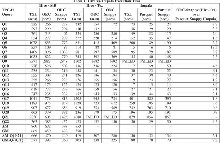
Table 1 presents the running time of the queries in Hive and Im-pala for each TPC-H query and for each file format that we exam-ined. The last column of the table presents the ratio between Hive-Tez’s response time over Impala’s response time for the snappy compressed ORC file and the snappy compressed Parquet format respectively. The table also contains the arithmetic (AM) and ge-ometric (GM) mean of the response times for all file formats. The values of AM-Q{9,21}and GM-Q{9,21}correspond to the arith-metic and geometric mean of all the queries but Query 9 and Query 21. Query 9 did not complete in Impala due to lack of sufficient memory and Query 21 did not complete in Hive-Tez when the ORC file format was used since a container was automatically killed by the system after the query ran for about2000seconds.

Figures 1 and 2 present an overview of the performance results for the TPC-H queries for the various file formats that we used, for both Hive and Impala. Figure 1 shows the normalized arithmetic mean of the response times for the TPC-H queries, and Figure 2 shows the normalized geometric mean of the response times; the 5_{Note that Hive-Tez includes some ORC file changes and hence} results in file size differences.

numbers plotted in Figures 1 and 2 are normalized to the response times of Impala when the snappy-compressed Parquet file format is used. These numbers were computed based on the AM-Q{9,21}

and GM-Q{9,21}values.

Figures 1 and 2 show that Impala outperforms both Hive-MR and Hive-Tez for all the file formats, with or without compression. Impala (using the compressed Parquet format) is about5X,3.5X, and 3.3X faster than Hive-MR and3.1X,2.3X and2,1X faster than Hive-Tez using TXT, uncompressed and snappy compressed ORC file formats, respectively, when the arithmetic mean is the metric used to compare the two systems. As shown in Table 1, the performance gains obtained in Impala vary from1.5X to13.5X.

An interesting observation is that Impala’s performance does not significantly improve when moving from the TXT format to the Parquet columnar format. Moreover, snappy compression does not further improve Impala’s performance when the Parquet file for-mat is used. This observation suggests that I/O is not Impala’s bottleneck for the majority of the TPC-H queries. On the other hand, Hive’s performance improves by approximately30%when the ORC file is used, instead of the simpler TXT file format.

From the results presented in this section, we conclude that Im-pala is able to handle TPC-H queries much more efficiently than Hive, when the workload’s working set fits in memory. As we will show in the following section, this behavior is attributed to the following reasons: (a) Impala has a far more efficient I/O sub-system than Hive-MR and Hive-Tez, (b) Impala relies on its own long running, daemon processes on each node for query execution and thus does not pay the overhead of the job initialization and scheduling introduced by the MapReduce framework in Hive-MR, and (c) Impala’s query execution is pipelined as opposed to Hive-MR’s MapReduce-based query execution which enforces data ma-terialization at each step.

We now analyze four TPC-H queries in both Hive-MR and Im-pala, to gather some insights into the performance differences. We also point out how query behavior changes for Hive-Tez.

3.5.1 Query 1

The TPC-H Query 1 is a query that scans thelineitemtable, applies an inequality predicate, projects a few columns, performs an aggregation and sorts the final result. This query can reveal how efficiently the I/O layer is engineered in each system and also demonstrates the impact of each each file format.

In Hive-MR, the query consists of two MapReduce jobs, MR1 and MR2. During the map phase, MR1 scans thelineitemtable, applies the filtering predicate and performs a partial aggregation. In the reduce phase, it performs a global aggregation and stores

(5)

Table 1: Hive vs. Impala Execution Time Hive - MR Hive - Tez Impala

TPC-H ORC ORC Parquet ORC-Snappy (Hive-Tez) Query TXT ORC Snappy TXT ORC Snappy TXT Parquet Snappy over

(secs) (secs) (secs) (secs) (secs) (secs) (secs) (secs) (secs) Parquet-Snappy (Impala) Q1 535 266 228 232 154 172 73 25 24 7.2 Q2 293 299 294 130 132 111 36 29 29 3.8 Q3 761 543 462 524 286 280 149 122 115 2.4 Q4 534 277 232 272 220 214 152 135 147 1.5 Q5 1078 833 772 831 415 409 200 189 190 2.2 Q6 357 109 85 114 88 81 15 6 6 13.5 Q7 1409 1096 1038 581 597 589 195 179 182 3.2 Q8 1085 822 770 743 392 369 155 140 148 2.5

Q9 3371 2883 2848 2102 1682 1692 FAILED FAILED FAILED –

Q10 778 526 502 336 236 224 117 59 50 4.5 Q11 235 234 216 158 141 134 30 22 22 6.1 Q12 555 308 241 226 186 184 37 38 40 4.6 Q13 255 266 228 176 155 156 119 123 127 1.2 Q14 417 175 155 124 123 120 17 13 14 8.6 Q15 619 272 233 166 159 156 27 21 22 7.1 Q16 247 235 239 152 143 133 39 44 43 3.1 Q17 1041 779 813 1205 945 724 401 385 395 1.8 Q18 1183 925 859 1128 723 672 259 185 189 3.6 Q19 907 677 656 919 734 569 742 703 710 0.8 Q20 663 379 332 236 179 175 196 195 191 0.9 Q21 2230 1605 1495 1688 FAILED FAILED 879 854 857 – Q22 363 385 452 123 132 130 50 29 30 4.3 AM 860 632 598 553 – – – – – – GM 665 459 422 358 – – – – – – AM-Q{9,21} 666 470 440 419 307 280 150 132 134 2.1 GM-Q{9,21} 577 393 360 303 238 225 90 70 70 3.2

Table 3: Time Breakdown for Query 1 in Hive-MR ORC TXT ORC Snappy (secs) (secs) (secs) MR1-map phase 485 215 176

MR1-reduce phase 5 7 4

MR2 10 11 11

the result in HDFS. MR2 reads the output produced by MR1 and sorts it. Table 3 presents the time spent in each MapReduce job, for the different file formats that we tested. As shown in the table, replacing the text format with the ORC file format, provides a 2.3X speedup. An additional speedup of 1.2X is gained by compressing the ORC file using the snappy compression algorithm.

Impala breaks the query into three fragments, namely F0, F1 and F2. F2 scans thelineitemtable, applies the predicate, and per-forms a partial aggregation. This fragment runs on all the compute nodes. The output of each node is shuffled across all the nodes based on the values of the grouping columns. Since there are4 dis-tinct value pairs for the grouping columns, only4compute nodes receive data. Fragment F1 merges the partial aggregates on each node and generates1row of data at each of the4compute nodes. Then, it streams the data to a single node that executes Fragment F0. This fragment merges all the partial aggregates and sorts the final result. Table 4 shows the time spent in each fragment. Frag-ment F0 is not included in the table, since its response time is in the order of a few milliseconds. As shown in the table, the use of the Parquet file improves F2’s running time by3.4X.

Table 4: Time Breakdown for Query 1 in Impala Parquet TXT Parquet Snappy (secs) (secs) (secs)

F1 2 3 3

F2 71 22 21

As shown in tables 3 and 4, Impala can provide significantly faster I/O read rates compare to Hive-MR. One main reason for this behavior, is that Hive-MR is based on the MapReduce framework for query execution, which in turn means that it pays the overhead of starting multiple map tasks when reading a large file, even when a small portion of the file needs to be actually accessed. For exam-ple, in Query 1, when the uncompressed ORC file format is used, 1872 map tasks (16 map task rounds) were launched to read a total of 196 GB. Hive-Tez avoids the startup overheads of the MapRe-duce framework and thus provides a significant performance boost. However, we observed that during the scan operation, both Hive-MR and Hive-Tez are CPU-bound. All the cores are fully utilized at all the machines and the disk utilization is less than20%. This observation is consistent with previous work [12]. The Java dese-rialization overheads become the bottleneck during the scan of the input files. However, switching to a columnar format helps reduce the amount of data that is deserialized and thus reduces the overall scan time.

Impala runs one impalad daemon on each node. As a result it does not pay the overhead of starting and scheduling multiple tasks per node. Impala also launches a set of scanner and reader threads

(6)

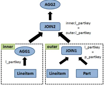
Figure 3: Query 17

on each node in order to efficiently fetch and process the bytes read from disk. The reader threads read the bytes from the underlying storage system and forward them to the scanner threads which parse them and materialize the tuples. This multi-threaded execution model is much more efficient than Hive-MR’s MapReduce-based data reading. Another reason, for Impala’s superior read perfor-mance over Hive-MR is that the Parquet files are generally smaller than the corresponding ORC files. For example, the size of the Parquet snappy compressedlineitemtable is196GB, whereas the snappy compressed ORC file is223GB on disk. During the scan, Impala is disk-bound with each disk being at least85% uti-lized. During this experiment, code generation is enabled in Im-pala. The impact of code generation for the aggregation operation is significant. Without code generation, the query becomes CPU-bound (one core per machine is fully utilized due to the single-threaded execution of aggregations) and the disks are under-utilized (<20%).

3.5.2 Query 17

The TPC-H query 17 is about2X faster in Impala than Hive-MR. Compared to other workload queries, like Query 22, this query does not get significant benefits in Impala.

Figure 3 shows the operations in Query 17. The query first applies a selection predicate on thepart table and performs a join between the resulting table and thelineitemtable (JOIN1). Thelineitemtable is aggregated on thel partkeyattribute (AGG1) and the output is joined with the output of JOIN1 again on thel partkeyattribute (JOIN2). Finally, a selection predicate is applied, the output is aggregated (AGG2) and the final result is pro-duced. Note that in this query one join operation (JOIN1) and one aggregation (AGG1) take as input thelineitemtable. Moreover, these operations as well as the final join operation (JOIN2) have the same partitioning key, namely l partkey.

MR2 12 11 11

Hive-MR’s “correlation” optimization [15] feature is able to iden-tify (a) the common input of the AGGR1 and JOIN1 operations and (b) the common partitioning key between AGG1, JOIN1 and JOIN2. Thus instead of launching a single MapReduce job for each of these operations, Hive-MR generates an optimized query plan that consists of two MapReduce jobs only, namely MR1 and MR2. In the map phase of MR1, thelineitemand part ta-bles are scanned, the selection predicates are applied and a partial aggregation is performed on thelineitemtable on the l partkey attribute. Note that because both JOIN1 and AGG1 get as input thelineitemtable, they share a single scan of the table. This provides a significant performance boost, since thelineitem ta-ble is the largest tata-ble in the workload, requiring multiple map task rounds when scanned. In the reduce phase, a global aggregation on thelineitemtable is performed, the two join operations are executed and a partial aggregation of the output is performed. This is feasible because all the join operations share the same partition-ing key. The second MapReduce job, MR2, reads the output of MR1 and performs a global aggregation. Table 5 presents the time breakdown for Query 17, for the various file formats that we used. We observed that Hive is CPU-bound during the execution of this query. All the cores are fully utilized (95%−100%), irrespective of the file format used. The disk utilization is less than5%.

Impala is not able to identify that the AGG1 and JOIN1 oper-ations share a common input, and thus scans thelineitem ta-ble twice. However, this does not have a significant impact in Impala’s overall execution time since during the second scan, the lineitemtables is cached in the OS file cache. Moreover, Im-pala avoids the data materialization overhead that occurs between the map and reduce tasks of Hive-MR’s MR1.

Table 6: Time Breakdown for Query 17 in Impala Parquet

TXT Parquet Snappy (secs) (secs) (secs)

F0 1 1 1

F1 33 24 24

F2 109 113 120

F3 249 240 248

F4 1 1 1

Impala breaks the query into 5 fragments (F0, F1, F2, F3 and F4). Fragment F4 scans theparttable and broadcasts it to all the compute nodes. Fragment F3 scans thelineitemtable, per-forms a partial aggregation on each node, and shuffles the results to all the nodes using the l partkey attribute as the partitioning key. Fragment F2 merges the partial aggregates on each node (AGG1) and broadcasts the results to all the nodes. Fragment F1 scans the lineitemtable and performs the join between this table and the parttable (JOIN1). Then, the output of this operation is joined with the aggregatedlineitemtable (JOIN2). The result of this join is partially aggregated and streamed to the node that executes Fragment F0. Fragment F0 merges the partial aggregates (AGG2) and produces the final result. Impala, executes both join operations using a broadcast algorithm, as opposed to Hive where both joins are executed in the reduce phase of MR1.

Table 6 presents the time spent on each fragment in Impala. As shown in the table, the bulk of the time is spent executing frag-ments F2 and F3. The output of thenmon6performance tool shows that during the execution of these fragments, only one CPU core is used and is100%utilized. This happens because Impala uses a

6

(7)

single thread per node to perform aggregations. The disks are ap-proximately10%utilized. We also observed that one core is fully utilized on each node, during the JOIN1 and JOIN2 operations. However, the time spent on the join operations (fragment F1) is low compared to the time spent in the AGG1 operation and thus the major bottleneck in this query is the single-threaded aggrega-tion operaaggrega-tion. For this reason, using the Parquet file format instead of the TXT format does not provide significant benefit.

In summary, the analysis of this query shows that Hive-MR’s “correlation” optimization helps shrinking the gap between Hive-MR and Impala on this particular query, since it avoids redundant scans on the data and also merges multiple costly operations into a single MapReduce job. This query does not benefit much from the Tez framework – the performance of Hive-Tez is comparable to that of Hive-MR. Although Hive-Tez avoids the task startup, scheduling and materialization overheads of MapReduce, it scans the lineitem table twice. Thus, Tez pipelining and container reuse do not lead to a significant performance boost in this particular query.

MR2 12 10 9

3.5.3 Query 19

As shown in Table 1, Query 19 is slightly faster in Hive than Impala. This query performs a join between thelineitemand parttables and then applies a predicate that touches both tables and consists of a set of equalities, inequalities and regular expres-sions connected with AND and OR operators. After this predicate is applied, an aggregation is performed.

TXT Parquet Snappy (secs) (secs) (secs)

F0 3 3 3

F1 610 590 600

F2 120 95 97

Hive-MR splits the query into two MapReduce jobs, namely MR1 and MR2. MR1 scans thelineitemandparttables in the map phase. In the reduce phase, it performs the join between the two tables, applies the filtering predicate, performs a partial aggregation and writes the results back to HDFS. MR2 reads the output of the previous job and performs the global aggregation.

Impala breaks the query into 3 fragments F0, F1, F2. Each node in the cluster executes fragments F1 and F2. Fragment F0 is ex-ecuted on one node only. Fragment F2 scans theparttable and broadcasts it to all the nodes. Fragment F1 first builds a hash table on theparttable. Then thelineitemtable is scanned and a hash join is performed between the two tables. During the join the complex query predicate is evaluated. The qualified rows are then partially aggregated. The output of fragment F1 is transmitted to the node that executes fragment F0. This node performs the global aggregation and produces the final result.

Tables 7 and 8 show the time breakdown for Query 19 in Hive-MR and Impala respectively, for the various file formats that we tested.

As shown in Table 8, fragment F2 which performs the scan of theparttable is slower when the data is stored in text format.

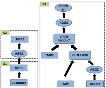
Figure 5: Query 22

The scan is about 1.2X times faster using the Parquet file format. During the execution of Fragment F2, all the cores are approxi-mately20%−30%utilized, and there is increased network activity due to the broadcast operation. The bulk of the query time is spent executing fragment F1. Using thenmonperformance tool, we ob-served that during the execution of the join operation only one CPU core is used on each node and runs at full capacity (100%). This is consistent with Impala’s limitation of executing join operations in a single thread. The output of Impala’sPROFILEstatement shows that the bulk of the time during the join is spent on probing the hash table using the rows from thelineitemtable and applying the complex query predicate.

As shown in Table 7, Hive-MR is much slower in reading the data from HDFS. As in Query 17, both Hive-MR and Hive-Tez are CPU-bound during the execution of this query. All the cores in each node are more than90%utilized and the disks are underuti-lized (<10%). The use of the ORC file has a positive effect since it can improve the scan time by 1.7X. However, in this particular query, Hive cannot benefit from predicate pushdown in the ORC file, because the filtering condition is a join predicate which has to be applied in the reduce phase of MR1. Hive-MR uses 120 reduce tasks to perform the join operation as well as the predicate evalua-tion, as opposed to Impala which uses 20 threads (one per compute node).

Table 9: Time Breakdown for Query 22 in Hive-MR ORC

TXT ORC Snappy (secs) (secs) (secs) S1 70 74 92

S2 31 34 41

S3 252 268 308

3.5.4 Query 22

Query 22 is the query with the most significant performance gain in Impala compared to Hive-MR (15X when using the snappy-compressed Parquet format).

Figure 5 shows the operations in Query 22. The query consists of 3 sub-queries in both Hive and Impala. The first sub-query (S1) scans thecustomertable, applies a predicate and materializes

(8)

0

200

400

600

800 1,000

1

2

3

4

5

6

7

8 10 11 12 13 14 15 16 17 18 19 20 21 22

Execution Time (secs)

TPC−H Query

Parquet(Codegen) Parquet(No Codegen)

Figure 4: Effectiveness of Impala Code Generation.

TXT Parquet Snappy (secs) (secs) (secs) S1 10 6 6

S2 2 2 2

S3 31 14 15

the result in a temporary table (TMP1). The second sub-query (S2) applies an inequality predicate on the TMP1 table, performs an ag-gregation (AGG1) and materializes the result in a temporary table (TMP2). The third sub-query (S3) performs an aggregation on the orderstable (AGG2). Then, an outer join between the result of AGG2 and table TMP1 is performed and a projection of the qual-ified rows is produced. In the following step, a cross-product be-tween the TMP2 table and the result of the outer join is performed, followed by an aggregation (AGG3) and a sort.

The time breakdown for Query 22 in Hive-MR is shown in Ta-ble 9. The response time of sub-queries S1 and S2 slightly in-creases when the ORC file is used, especially if it is compressed. These queries materialize their output in temporary tables. The output size is small (e.g., 803 MB in text format for sub-query S1). The overhead of creating and compressing an ORC file for such a small output has a negative impact on the overall query time. The bulk of the time in sub-query S3 is spent executing the outer join using a full MapReduce job. The cross-product, on the other hand, is executed as a map-side join in Hive. Our analysis shows that the time difference between the TXT format and the snappy-compressed ORC file is due to increased scan time of the two tables participating in the outer join operation because of decompression overheads. In fact, for this particular operation the scan time of the tables stored in compressed ORC file format increases by28% compared to the scan time of tables in uncompressed ORC file. Hive-MR uses 7 MapReduce jobs for this query. All had similar behavior: when a core is used during the query execution, it is fully utilized whereas the disks are underutilized (< 15%). Hive-Tez avoids the startup and materialization overheads of the MapReduce jobs and thus improves the running time by about3.5X.

The time breakdown for Query 22 in Impala is shown in Ta-ble 10. As shown in the taTa-ble Impala is faster than Hive-MR in each sub-query, with speedups ranging from7X to20.5X depend-ing on the file format. This performance gap is mainly attributed to the fact that Impala has a more efficient I/O subsystem. This behavior is observed in sub-queries S1 and S2 which only include scan operations. The disks are fully utilized (>90%) during the

scan operation as well as during the materializion of the results. The CPU utilization was less than20%on each node. Note that the startup cost of sub-query S3 and the time spent in code genera-tion constitute about30%of the query time, which is a significant overhead. This is because these queries scan and materialize very small amounts of data. Impala breaks sub-query S3 into 7 frag-ments. The ImpalaPROFILEstatement shows that I/O was very efficient for that sub-query too. For example, Impala spent13 sec-onds to read and partially aggregate theorders table (AGG2) when the TXT format was used corresponding to70M B/secper disk on each node. During the scan operation all the CPU cores were10% utilized. The cross-product and outer join operations were executed using a single core (100%utilized). However, the amount of data involved in these operations is very small and thus the single-threaded execution did not become a major bottleneck for this sub-query. Both Impala and Hive picked the same algo-rithms for these operations, namely a partitioned-based algorithm for the outer join and a broadcast algorithm for the cross-product.

3.6 Effectiveness of Runtime Code Generation

in Impala

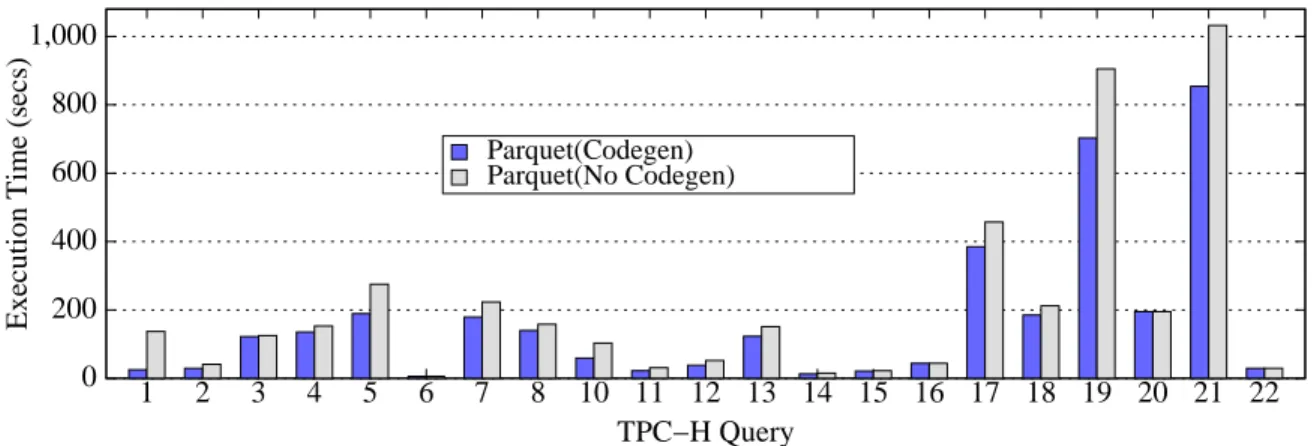
One of the much touted features of Impala is its ability to gen-erate code at runtime to improve CPU efficiency and query exe-cution times. Impala uses runtime code generation for eliminating various overheads associated with virtual function calls, inefficient instruction branching due to large switch statements, etc. In this section, we conduct experiments to evaluate the effectiveness of runtime code generation for the TPC-H queries. We again use the 21 TPC-H queries (Query 9 fails), execute them sequentially, with and without runtime code generation and measure the overall exe-cution time. The results are presented in Figure 4.

With runtime code generation enabled, the query execution time improves by about1.3for all the queries combined. As Figure 4 shows, runtime code generation has different effects for different queries. TPC-H Query 1 benefits the most from code generation, improving by5.5X. The remaining queries see benefits up to1.75X. As discussed in Section 3.5, Query 1 scans thelineitem ta-ble and then performs a hash-based aggregation. Impala’s output of thePROFILEstatement shows that the time spent in the ag-gregation increases by almost6.5X when runtime code generation is not enabled. During the hash-based aggregation, for each tuple the grouping columns (l returnflagsand l linestatus) are evaluated and then hashed. Then a hash table lookup is per-formed and all the expressions used in the aggregation (sum,avg andcount) are evaluated. Runtime code generation can help

(9)

0

100

200

300

400

500

600

700

800

900

3

7

19

27

34

42

43

46

52

53

55

59

63

65

68

73

79

89 98 ss_max

Execution Time (secs)

TPC−DS Inspired Query

Hive−MR Hive−Tez Impala

Figure 6: TPC-DS inspired Workload 1

nificantly improve the performance of this operation as all the logic for evaluating batches of rows for aggregation is compiled into a single inlined loop. Code generation does not practically impose any performance overhead. For example, the total code generation time for Query 1 is approximately400ms.

From the results presented in Figure 4, we conclude that runtime code generation generally improves overall performance. However, the benefit of code generation varies for different queries. In that respect, our findings are inline with what has been reported7_.

3.7 TPC-DS Inspired Workloads

In this section, we present cluster experiments using a workload inspired by the TPC-DS benchmark8. This is the workload pub-lished by Impala developers9 where they compare Hive-MR and Impala on the cluster setup described in [22]. Our goal is to re-produce this experiment on our hardware and examine if the per-formance trends are similar to what is reported in [22]. We also performed additional experiments using Hive-Tez. Note that in our experimental setup we use 20 compute nodes connected through a 10Gbit Ethernet switch as opposed to the setup used by the Impala developers which consists of 5 compute nodes connected through a 1Gbit Ethernet switch. Our nodes have similar memory and I/O configurations with the node configuration described in [22] but contain more physical cores (12 cores instead of 8 cores).

The workload (TPC-DS inspired workload 1) consists of 20 queries which access a single fact table and six dimension ta-bles. Thus, it significantly differs from the original TPC-DS bench-mark that consists of 99 queries that access 7 fact tables and mul-tiple dimension tables. Since Impala does not currently support windowing functions and rollup, the TPC-DS queries have been modified by the Cloudera developers to exclude these features. An explicit partitioning predicate is also added, in order to restrict the portions of the fact table that need to be accessed. In the official TPC-DS benchmark, the values of the filtering predicates in each query change with the scale factor. Although Cloudera’s work-load operates on 3 TB TPC-DS data, the predicate values do not match the ones described in the TPC-DS specification for this scale factor. For completeness, we also performed a second experiment

7 http://blog.cloudera.com/blog/2013/02/inside-cloudera-impala-runtime-code-generation/ 8 http://www.tpc.org/tpcds/ 9 https://github.com/cloudera/impala-tpcds-kit

which uses the same workload but removes the explicit partition-ing predicate and also uses the correct predicate values (TPC-DS inspired workload 2).

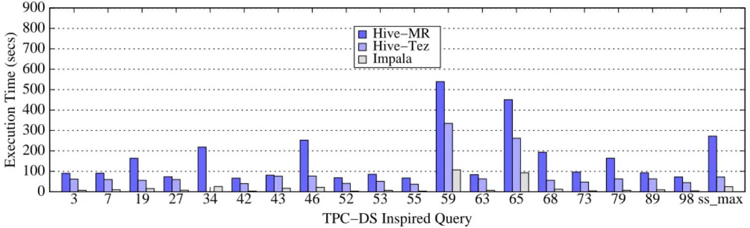
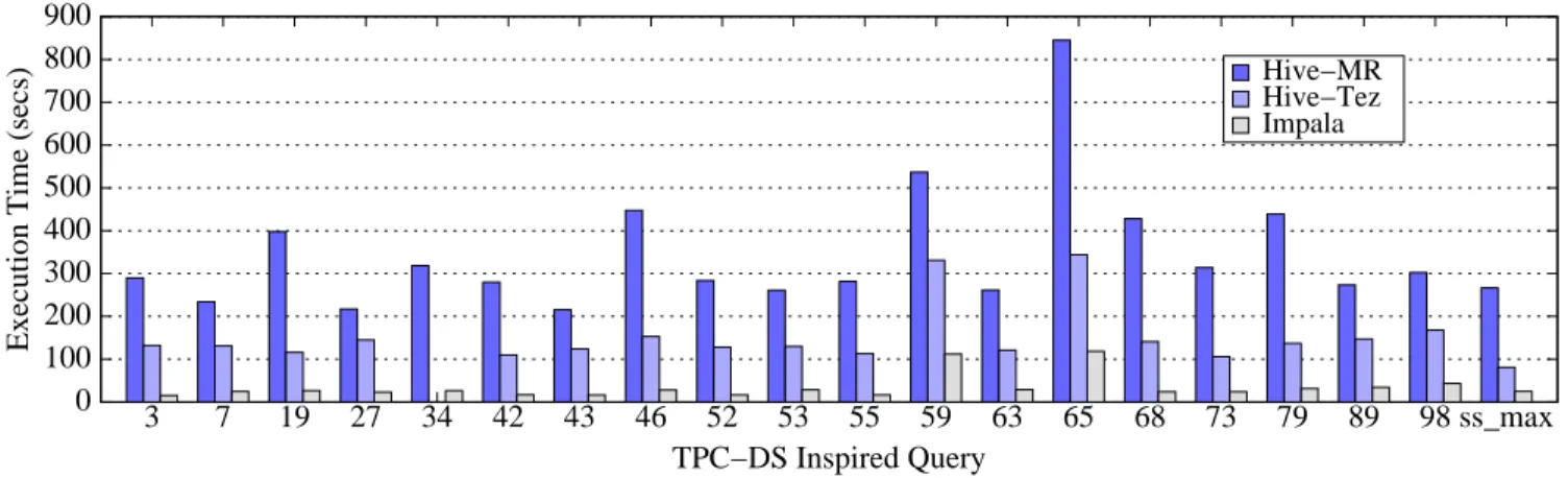
As per the instructions in [22] we stored the data in Parquet and ORC snappy-compressed file formats. We flushed the file cache before running each workload. We repeated each experiment three times and report the average execution time for each query. As in the previous experiments, we computed statistics on the Impala ta-bles. The Hive-MR configuration used by the Impala developers is not described in [22] so we performed our own Hive-MR tuning. More specifically we enabled map-side joins, predicate pushdown and the “correlation” optimization in Hive-MR and also the vector-ized execution in Hive-Tez. Figures 6 and 7 present the execution times for the queries ofTPC-DS inspired workload 1and theTPC-DS inspired workload 2, respectively.

Our results show that Impala is on average8.2X faster than Hive-MR and4.3X faster than Hive-Tez on theTPC-DS inspired workload 1and10X faster than Hive-MR and4.4X faster than Hive-Tez on theTPC-DS inspired workload 2. These num-bers show the advantage of Impala for workloads that access one fact table and multiple small dimension tables. The query execution plan for these queries has the same pattern: Impala broadcasts the small dimension tables where the fact table data is and joins them in a pipelined fashion. The performance of Impala is also attributed to its efficient I/O subsystem. In our experiments we observed that Hive-MR has significant overheads when ingesting small tables, and all these queries involve many small dimension tables. When Hive-MR merges multiple operations into a single MapReduce job the performance gap between the two systems shrinks. For exam-ple, in Query 43, Hive-MR performs three joins and an aggregation using one MapReduce job. However, it starts multiple map tasks to scan the fact table (one per partition) which are CPU-bound. The overhead of instantiating multiple task rounds for a small amount of data makes Hive-MR almost 4X slower than Impala on this query in theTPC-DS inspired workload 1. Hive-MR is 13X slower than Impala for Query 43 of TPC-DS inspired workload 2. Since the explicit partitioning predicate is now removed, Hive-MR scans all the partitions of the fact table using one map task per partition, resulting in a very large number of map tasks. When Hive-MR generates multiple MapReduce jobs (e.g., in Query 79), the performance gap between Hive-MR and Impala increases. The performance difference between Hive and Impala decreases when Tez is used. This is because Impala and Hive-Tez avoid Hive-MR’s scheduling and materialization overheads.

(10)

0

100

200

300

400

500

600

700

800

900

3

7

19

27

34

42

43

46

52

53

55

59

63

65

68

73

79

89 98 ss_max

Execution Time (secs)

TPC−DS Inspired Query

Hive−MR Hive−Tez Impala

Figure 7: TPC-DS inspired Workload 2

It is worth noting that Hive has support for windowing functions and rollup. As a result 5 queries of this workload (Q27, Q53, Q63, Q89, Q98) can be executed using the official versions of the TPC-DS queries in Hive but not in Impala. We executed these 5 official TPC-DS queries in Hive and observed that the execution time in-creases at most by10%compared to the queries in workload 2.

To summarize, we observe similar trends in both TPC-H and TPC-DS inspired workloads. Impala performs better for TPC-DS inspired workloads than the TPC-H like workload because of its specialized optimizations for the query pattern in the workloads (joining one large table with a set of small tables).

The individual query speedups that we observe (4.8X to23X) are not as high as the ones reported in [22] (6X to69X) but our hard-ware configurations differ and it is not clear whether we used the same Hive-MR configuration when running the experiments and whether Hive-MR was properly tuned in [22], since these details are not clearly described in [22].

4. MICRO-BENCHMARK RESULTS

In this section, we study the I/O characteristics of Hive-MR and Impala over their columnar formats, using a set of micro-benchmarks.

4.1 Experimental Environment

We generated three data files of 200 GB each (in text format). Each dataset contains a different number of integer columns (10, 100 and 1000 columns). We used the same data type for each col-umn in order to eliminate the impact of diverse data types on scan performance. Each column is generated according to the TPC-H specification for the l partkey attribute. We preferred to use the TPC-H generator over a random data generator because both the Parquet and the ORC file formats use run-length encoding (RLE) to encode integer values in each column. Thus, datasets with arbi-trary random values would not be able to exploit this feature.

For our micro-benchmarks, we use one “control” node that runs all the main processes used by Hive, Hadoop and Impala, and a second “‘compute” node to run the actual experiments. For the Hive-MR experiments, we use the default ORC file stripe size (256 MB) unless mentioned otherwise. During the load phase, we use only 1 map task to convert the dataset from the text format to the ORC file format in order to avoid generating many small files which can negatively affect the scan performance. In all our experiments, the datasets are uncompressed, since our synthetic datasets cannot significantly benefit from block compression codecs.

4.2 Scan Performance in Hive and Impala

In this experiment, we measure the I/O throughput while scan-ning data in Hive-MR and Impala in a variety of settings. More specifically, we vary: (a) the number of columns in the file, (b)the number of columns accessed, and (c) the column access pattern.

In each experiment, we scan a fixed percentage of the columns and record the read throughput, measured as the amount of data

processed by each system, divided by the scan time. We

experi-mented with two column access patterns, namelysequential(S) andrandom(R). GivenNcolumns to be accessed, in the sequen-tial access pattern we scan the columns starting from the1st_{up to} theNth

one. In the random access pattern, we randomly pickN

columns from the file and scan those. As a result, in the random ac-cess pattern, data skipping may occur between column acac-cesses. To scan columnsC1,...,CNwe issue a “selectmax(c1), ...,max(cN) from table” query in both Impala and Hive-MR. We preferred to use

max()overcount(), sincecount()queries without a filtering predicate are answered using metadata only in Impala.

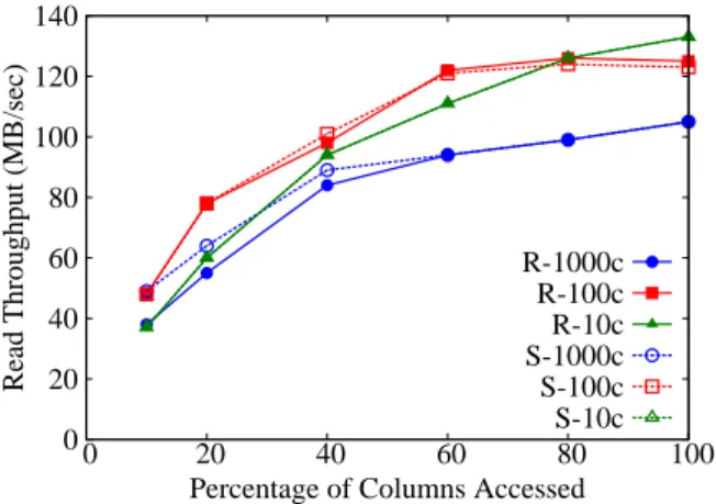
Figures 8 and 9 present the I/O throughput in Impala and Hive-MR respectively, as the percentage of accessed columns varies from 10%to100%, for both thesequential(S)and therandom(R) access patterns using our three datasets. Our calculations do not in-clude the MapReduce job startup time in Hive-MR. When using the 1000-column file and accessing more than60%of the columns, Impala pays a 20-30 seconds compilation cost. This time is also not included in our calculations.

As shown in Figure 8, the Impala read throughput for the datasets that consist of 100 and 1000 integer columns, remains almost con-stant as we vary the percentage of columns accessed using the sequentialaccess pattern. There are two interesting observa-tions on thesequentialaccess pattern: (a) the read throughput on the 1000-column dataset is lower than that of the 100-column dataset, and (b) the read throughput on the 10-column dataset in-creases as the number of accessed columns inin-creases.

Regarding the first observation, we noticed that the average CPU utilization when scanning a fixed percentage of columns is higher when scanning the 1000-column file than when scanning the 100-column file. For example, when scanning 60% of the 100-columns in the dataset, the CPU utilization is 94% during the experiment with the 1000-column file and 67% during the experiment with the 100-column file. Using the ImpalaPROFILEstatement, we observed that the ratio of the time spent in parsing the bytes to the time spent in actually reading the bytes from HDFS is higher for the 1000-column file than the 100-1000-column file. Although the amount of data

(11)

0 200 400 600 800 1000 0 20 40 60 80 100

Read Throughput (MB/sec)

Percentage of Columns Accessed R-1000c R-100c R-10c S-1000c S-100c S-10c 0 20 40 60 80 100 120 140 0 20 40 60 80 100

Read Throughput (MB/sec)

Percentage of Columns Accessed R-1000c R-100c R-10c S-1000c S-100c S-10c

Figure 8: Impala/Parquet Read Throughput Figure 9: Hive/ORC Read Throughput

processed is similar in both cases, processing a 1000-column record is more expensive than processing a 100-column record.

Our 3 datasets have the same size in text format but different record sizes (depending on the number of columns in the file). The fact that the 10-column file contains more records than the other files, is the reason why the read throughput for this file increases as the number of accessed columns increases. More specifically, tuple materialization becomes a bottleneck when scanning data from this file, especially when the amount of data accessed is small. When a few columns are accessed, the cost of tuple materialization domi-nates the running time. To verify this, we repeated the same exper-iment but added a predicate of the form “c1 <0ORc2 <0OR ... ORcN<0” in the query. This predicate has0%selectivity but still forces a scan of the necessary columns. Now, the read through-put in thesequentialaccess pattern becomes almost constant as the number of accessed columns varies.

As shown in Figure 8, when the access pattern israndom, the read throughput increases as the number of accessed columns in-creases and it is typically lower then the corresponding throughput of thesequentialaccess pattern. This observation is consistent with the HDFS design. Scanning sequentially large amounts of data from HDFS is a “cheap” operation. For this reason, as the percent-age of columns accessed increases, the read throughput approaches the throughput observed in thesequentialaccess pattern.

Regarding our Hive-MR experiments, Figure 9 shows that the behavior of the system is independent of the access pattern ( sequen-tial or random). The read throughput always increases as the number of accessed columns increases. This behavior is attributed to the high overhead of starting and running short map tasks. As an example, scanning only one column from the 1000-column file takes about120seconds. Scanning sequentially 100 columns from the same file takes about170 seconds. In our case, each map task processes512 MB of data (aka, two ORC stripes). Since our datasets have sizes of about 80-90 GB, each file scan translates into multiple map rounds. Moreover, the average CPU utilization during the Hive-MR experiments is87%and the disks are under-utilized (<30%). This behavior is closely related to the overheads introduced by object deserialization in java [12]. The CPU over-heads introduced when scanning a large number of records (10-column file) increase each map task’s time by23%.

The last property of the file formats that we tested is efficient skipping of data when the access pattern israndom. To measure the amount of data read from disk, we used thenmonperformance tool. We observed that Hive-MR and Impala read almost as much data as needed during the experiments with the 10-column and 100-column files. Efficient data skipping is more challenging in the

case of the 1000-column dataset. In the worst case, Impala reads twice as much data as needed on this dataset. Hive-MR, is not able to efficiently skip columns even when accessing only10%of the dataset’s columns and ends up reading about92%of the file. Note that the unnecessary prefetched bytes are not deserialized. Thus the impact of prefetching on the overall execution time is not signifi-cant. Since packing1000columns within a256MB stripe results in unnecessary data prefetching, we increased the ORC stripe size to750MB and repeated the experiment. In this experiment, Hive-MR reads as much data as needed. In this case, each column is allocated more bytes in the stripe, and as a result skipping very small chunks of data is avoided.

4.3 Effectiveness of Indexing in ORC File

When a selection predicate on a column is pushed down to the ORC file, the built-in index can help skip chunks of data within a stripe based on theminandmaxvalues of the column within the chunk. A column chunk can either be skipped or read as a whole. Thus, the index operates on a coarse granularity as opposed to fine-grained indices, such as B-trees. In this experiment, we examine the effectiveness of the lightweight built-in index in ORC file.

We use two variants of the 10-column dataset, namelysorted andunsorted. More specifically, we picked one columnCand sorted the dataset on this column to create thesortedvariant. For both datasets, we execute the following query: “selectmax(C)

from table whereC < s”. The parametersdetermines the selec-tivity of the predicate. We enable predicate pushdown and index filtering and use the default index row group size of 10,000 rows.

Figure 10 shows the response time of the query in Hive-MR as the predicate becomes less selective, for thesortedand the unsorteddatasets. Figure 11 shows the amount of data

pro-cessed for each selectivity factor over the amount of data propro-cessed

at the100% selectivity factor, for both the unsortedand the sorteddatasets. At the 100%selectivity point, Hive-MR pro-cesses approximately8GB of data when the dataset is unsorted, which corresponds to one full column. In the case of thesorted dataset,344MB of data is processed. This is because, in the sorted case, run-length encoding can further compress the column’s data.

As shown in the figures, the built-in index in ORC file is helpful only when the selectivity of the predicate is0%for theunsorted dataset. In this case, only 11.7 MB of data out of the 8 GB is actually processed by Hive-MR. This is expected since all the row groups of the file can immediately be skipped. However, when the predicate is less selective (even just1%) the whole column is actually read. We repeated the same experiment but reduced the row group size to the minimum allowed value of 1,000 rows. Even

(12)

0

50

100

150

200

250

300 0%

1%

5%

10%

50%

100%

Scan Time (secs)

Predicate Selectivity

ORC (sorted) ORC (unsorted)

0%

20%

40%

60%

80%

100%

120%

0%

1%

5%

10%

50%

100%

Data Processed

Predicate Selectivity

ORC (sorted) ORC (unsorted)

Figure 10: Predicate Selectivity vs. Scan Time Figure 11: Predicate Selectivity vs. Data Processed

in this case, the index is not helpful for predicate selectivities above 0%for theunsorteddataset. Note that the running time of the query increases as the predicate becomes less selective. This is expected, since more records need to be materialized.

On the other hand, the built-in index is more helpful when the column is sorted. In this case, the range of values in each row group is more distinct, and thus the probability of a query predicate falling into a smaller number of row groups increases. The amount of data processed and the response time of the query gradually increase as the predicate becomes less selective. As shown in Figure 11, the full column is read only at the100%selectivity factor.

Our results suggest that the built-in index in ORC file is more useful when the data is sorted in advance or has a natural order that would enable efficient skipping of row groups.

5. CONCLUSIONS

Increased interest in SQL-on-Hadoop fueled the development of many SQL engines for Hadoop data. In this paper, we con-duct an experimental evaluation of Impala and Hive, two repre-sentatives among SQL-on-Hadoop systems. We find that Impala provides a significant performance advantage over Hive when the workload’s working set fits in memory. The performance differ-ence is attributed to Impala’s very efficient I/O sub-system and to its pipelined query execution which resembles that of a shared-nothing parallel database. Hive on MapReduce pays the overhead of scheduling and data materialization that the MapReduce frame-work imposes whereas Hive on Tez avoids these overheads. How-ever, both Hive-MR and Hive-Tez are CPU-bound during scan op-erations, which negatively affects their performance.

6. ACKNOWLEDGMENTS

We thank Simon Harris and Abhayan Sundararajan for providing the TPC-H and the TPC-DS workload generators to us.

7. REFERENCES

[1] D. J. Abadi, P. A. Boncz, and S. Harizopoulos. Column oriented Database Systems. PVLDB, 2(2):1664–1665, 2009.

[2] A. Abouzeid, K. Bajda-Pawlikowski, D. J. Abadi, A. Rasin, and A. Silberschatz. HadoopDB: An Architectural Hybrid of MapReduce and DBMS Technologies for Analytical Workloads. PVLDB, 2(1):922–933, 2009.

[3] A. Ailamaki, D. J. DeWitt, and M. D. Hill. Data Page Layouts for Relational Databases on Deep Memory Hierarchies. VLDB J., 11(3):198–215, 2002.

[4] Apache Drill.http://www.mapr.com/resources/ community-resources/apache-drill. [5] Apache Hadoop.http://hadoop.apache.org/. [6] Apache Hive.http://hive.apache.org/. [7] Apache Shark.http://shark.cs.berkeley.edu/. [8] Apache Spark.https://spark.incubator.apache.org/. [9] L. Chang et al. HAWQ: A Massively Parallel Processing SQL Engine

in Hadoop. In ACM SIGMOD, pages 1223–1234, 2014. [10] Cloudera Impala.

http://www.cloudera.com/content/cloudera/en/ products-and-services/cdh/impala.html. [11] D. J. DeWitt, R. V. Nehme, S. Shankar, J. Aguilar-Saborit,

A. Avanes, M. Flasza, and J. Gramling. Split Query Processing in Polybase. In ACM SIGMOD, pages 1255–1266, 2013.

[12] A. Floratou, J. M. Patel, E. J. Shekita, and S. Tata. Column-oriented Storage Techniques for MapReduce. PVLDB, 4(7):419–429, 2011. [13] A. Floratou, N. Teletia, D. J. DeWitt, J. M. Patel, and D. Zhang. Can

the Elephants Handle the NoSQL Onslaught? PVLDB, 5(12):1712–1723, 2012.

[14] Y. He, R. Lee, Y. Huai, Z. Shao, N. Jain, X. Zhang, and Z. Xu. RCFile: A Fast and Space-efficient Data Placement Structure in MapReduce-based Warehouse Systems. In ICDE, pages 1199–1208, 2011.

[15] R. Lee, T. Luo, Y. Huai, F. Wang, Y. He, and X. Zhang. YSmart: Yet Another SQL-to-MapReduce Translator. In ICDCS, pages 25–36, 2011.

[16] S. Melnik, A. Gubarev, J. J. Long, G. Romer, S. Shivakumar, M. Tolton, and T. Vassilakis. Dremel: Interactive Analysis of Web-scale Datasets. PVLDB, 3(1-2):330–339, 2010. [17] Presto.http://prestodb.io/.

[18] M. Stonebraker, D. J. Abadi, A. Batkin, X. Chen, M. Cherniack, M. Ferreira, E. Lau, A. Lin, S. Madden, E. O’Neil, P. O’Neil, A. Rasin, N. Tran, and S. Zdonik. C-Store: A Column-oriented DBMS. In PVLDB, pages 553–564, 2005.

[19] M. Stonebraker, D. J. Abadi, D. J. DeWitt, S. Madden, E. Paulson, A. Pavlo, and A. Rasin. MapReduce and parallel DBMSs: Friends or Foes? CACM, 53(1):64–71, 2010.

[20] Tajo.http://tajo.incubator.apache.org/. [21] A. Thusoo, J. S. Sarma, N. Jain, Z. Shao, P. Chakka, N. Zhang,

S. Anthony, H. Liu, and R. Murthy. Hive - a Petabyte Scale Data Warehouse using Hadoop. In ICDE, pages 996–1005, 2010. [22] TPC-DS like Workload on Impala.

http://blog.cloudera.com/blog/2014/01/ impala-performance-dbms-class-speed/. [23] Trevni Columnar Format.http:

//avro.apache.org/docs/1.7.6/trevni/spec.html. [24] R. S. Xin, J. Rosen, M. Zaharia, M. J. Franklin, S. Shenker, and

I. Stoica. Shark: SQL and Rich Analytics at Scale. In ACM SIGMOD, pages 13–24, 2013.