Towards Application of a Parallel, High Order Discontinuous Galerkin
Method for Reacting Flow Simulations
Amjad Ali1, Ahmad Hassan1, Khalid S. Syed1, Muhammad Ishaq1 and Idrees Ahmad2
1. CASPAM, Bahauddin Zakariya University, Multan (60800), Pakistan. Email: [email protected] 2. Pakistan Institute of Engineering and Applied Sciences, P. O. Nilore, Islamabad, Pakistan.
Abstract
An accurate numerical technique for the numerical simulation of 1D reacting flow problems is implemented. The technique is based on nodal discontinuous Galerkin finite element method that makes use of high order approximating polynomials within each element to capture the physics of reacting flow phenomena. High performance computing is achieved through parallelization of the computer code using MPI to run on any distributed memory parallel computing architecture. The developed parallel code is tested on a PC with modern multicore CPUs, and on a multi-node compute cluster made up of commodity PC hardware, having gigabit Ethernet as the interconnect. The results presented are in good agreement with those available in the literature.
Key Words
: reacting flows; nodal discontinuous Galerkin method; parallel computing; multicore CPU1. Introduction
Computational Fluid Dynamics (CFD) is extremely useful and promising way to forecast or reconstruct the behavior of certain engineering products or physical situations through numerical simulations. Most of the physical experiments might be impossible to be carried out, expensive to be performed or less insight providing. The simulations, on the other hand, are more likely to be carried out, lesser expensive to be performed and provide more insight and comprehensive information. CFD simulations reduce the number of required experiments during development and testing of new products. For example, the number of wind-tunnel hours required for the development of Boeing-747 aircraft (in 1963) was reduced by a factor of 10 for Boeing-767 (in 1982) and was further reduced by another factor of 10 for Boeing-777 (in 1998). The main enabling factors for so impressive developments in CFD during past three decades are enormous growth in computing capabilities, steep decline in computing cost and development of more and more efficient algorithms [1].
In CFD, the simulation of flows often requires solving partial differential equation (PDEs) numerically. Common methods used for numerical
solution of PDEs are Finite Difference Methods (FDM), Finite Volume Methods (FVM) and Finite Element Methods (FEM). Yet there is another class of methods, Discontinuous Galerkin Finite Element Methods (DG-FEM or simply DGM), also referred to as hybrid FEM/FDM/FVM methods. DGM combines a number of benefits and overcomes a number of weaknesses of finite element and finite volume methods. In DGM, the solution is approximated by high order polynomials within each cell (like in FEM) but without the global continuity requirement, while the physics of wave propagation is accounted for by using some numerical flux scheme (like in FVM) to cope with discontinuous representation of the solution at element interfaces. In principle, the accuracy in DGM is achieved by the high order local polynomial approximations and the stability is achieved by careful selection of flux scheme.
Absence of global continuity requirement of the solution, i.e., independency of polynomial approximation in an element from that of other elements, makes DGM very compact. This feature, in conjunction with some other desired numerical properties, makes DGM very flexible so that it allows easy handling of a vast range of cell types and mesh topologies. It allows the use of adaptive techniques (like h- and p- refinements). It also supports easy implementation of certain strategies for solver
acceleration, in both serial and parallel programming environments. A comparison of generic properties of these methods is given in Table 1, adapted from [2]. In Table 1, „Y‟ means that the method is capable, „N‟ means that the method has shortcoming, and „Q‟ means that the method is capable but with modification and is not a preferred choice.
Discontinuous Galerkin Method has recently gained popularity for the solution of systems of conservation laws on unstructured grids. However several issues of DGM need to be addressed. These issues include high CPU/memory requirements (compared to FVM or High Order FDM) because of increase in number of degrees of freedom, and oscillations in presence of strong discontinuities. DGM is also low tolerant to its under-resolved features. The challenge is to make DG competitive, or at least compliment, to the well established schemes for real-world problems. Some accounts of history and developments of DGMs can be found in [2,3]. Some significant landmark DGM formulations are [4-14].
Table 1: A comparison of spatial discretization schemes
FDM FVM FEM DGM
Complex Geometry N Y Y Y
Higher Order Accuracy and Adaptivity
Y N Y Y
Compactness N N Y Y
Explicit Semi
Discrete Form Y Y N Y
Conservation Laws Y Y Q Y
Elliptic Problems Y Q Y Q
A basic problem in CFD is to develop accurate and efficient solvers for the simulation of reacting flows. Reacting flows are characterized by the presence of multiple scales, including reaction fronts, boundary layers and shocks. It is possible for the reaction front to move at some velocity other than the velocity of the fluid and the moving fronts may be
sharp, as well. The numerical method should be capable of accurately resolving such flows. The numerical methods mostly used for such problems are adaptive, especially with moving finite elements or moving grid [15-20]. In the present paper, instead of using some adaptive technique, the objective of our work is to apply DGM with high order approximating polynomials locally within each element to perform numerical simulation of reacting flows. We solve three selected reacting flow problems, two from flame propagation in combustion and one from mathematical biology, using a discontinuous Galerkin method that is based on so-called „nodal‟ approach [2]. Section 2 of this paper presents the nodal discontinuous Galerkin method.
Our next contribution in this paper is to develop a parallel solution of our serial nodal discontinuous Galerkin code to run on a parallel computing architecture. We also perform scalability analysis of our parallel code on a number of parallel computing machines, including a PC with 8 processing cores, and a cluster of PCs. For parallelization, we use Message Passing Interface (MPI) library [21]. MPI is a scalable parallel programming standard specially developed for distributed memory parallel machines. It has evolved as a de facto industry standard for message passing programming. A number of MPI implementations have been created, which include both open-source (free) and commercial ones. Keeping in view our problem sizes and the algorithm, we tested our parallel code on a standalone PC with multicore CPUs and on a small multi node cluster PCs. Clusters of PCs are composed of commonly available hardware components [22]. Therefore they are experienced as a very cost effective solution for parallel computing. They are also sometimes called Beowulf clusters. Section 3 describes the parallelization platforms, software‟s and strategies used in the present work. Section 4 lists our selected example problems and Section 5 consists of results and discussion. Section 6 gives the conclusions.
2. The Nodal Discontinuous Galerkin
Scheme for 1D Diffusion Equations
In the current work, the nodal version of discontinuous Galerkin finite element method is used, as described in [2]. The governing equations of reacting flow problems considered in this studyconstitute systems of 1D diffusion equations. Here we give DGM formulation of a general 1D diffusion equation with stiff source term that can be used for high order discretization of 1D diffusion equations. This equation can be expressed as,
au u
gu x x
t
, x
L,R (1)For approximating the solution of PDEs involving high order spatial derivatives by DGM, first rewrite the high order spatial derivative as a system of first order ordinary differential equations (ODEs). For this, we introduce a new variable,
u u, aq x (2)
and rewrite (1) as follows:
. 0 u u a q u g q u a u x x t (3)For the discretization of the above system with the DGM usually called Local DGM for (1), we divide the domain into K disjoint, non-overlapping elements, Dk, such that,
,
1 k K kD
(4)where
denotes the direct sum. We define a global space Vhfor the test functions as,k h K k h
V
V
1 (5) where k hV is a local space generated by Nth degree polynomials i,i1,2,,Np, defined on the
elements, Dk. NpN1 is the number of grid points in Dk used for constructing interpolating polynomials
i. We seek to obtain an approximation (uhk,qhk) to
) ,
(u q such that both k h k
h q
u and belong to the finite dimensional space, k
h
V . Now multiplying (3) with arbitrary test function n and integrating over the element Dk, we get, after performing integration by parts,
ˆ
,
Dk
n k h k D n k h k D n x k h k D n k h t dx u g dx q a n dx q a dx u (6)
ˆ
0,
Dk
n k h k D n x k h k D n k h dx u a n dx a u dx q (7)
where Dk is the boundary of Dk, and (ˆ ( k))
h
q a
n and
)) ( ˆ ( k h u a
n are fluxes across the element in the unit normal direction,nˆ, to the boundary. These fluxes are replaced by suitably chosen numerical fluxes denote by(ˆ( k))
h
q a
n and(ˆ( k))
h
u a
n in (6) and (7) and lead to the following weak form of (3) on each element, Dk:
,ˆ 0
k D n k h k D n k h n x k h n k h t dx q a n dx u g q a u (8)
.ˆ 0
k D n k h k D n x k h n k h dx u a n dx a u q (9)The above equations give DGM formulation of (3) in weak form. It requires test functions to be smooth. In situations where non-smooth test functions are to be used, we may employ strong form of DGM formulation which is obtained by integrating by parts of (8) and (9) once again:
,ˆ 0
k D n k h k h k D n k h k h x k h t dx q a q a n dx u g q a u (10)
.ˆ 0
k D n k h k h k D n k h x k h dx u a u a n dx u a q (11)In the nodal implementation of DGM, k h k h q
u , and the source term
kh
u
, , , , , x q u x t x q t x u t x q t x u k i Npi ik k i k
i Np
i kh i i k h k h k h
1 1 (12)
u g
u g
x,t x g
x,g k i Np i k i k i Np i i k h k h k h k
h
1 1 (13)
where k
xi
are N-th order Lagrange polynomials on k
D and form basis of k h
V . In present work we employ strong form given by (10) and (11). Use of (12) and (13) in (10) and (11) leads to the following system of differential algebraic equations,
, ˆ ~
k D k k h k h k h k k h k h k dx x q a q a M S t d d M L n g q u (14)
, ˆ
k D k k h k h k h k h k dx x u a u a SM q u n L (15)
Where
k D k j k i k ij dxM (16)
is the mass matrix,
k k D k j x k i ij D k j x k i ijdx
a
S
dx
a
S
~
(17)are the stiffness matrices,
k
T Np k kh u1,,u
u ,
k
TNp k k
h q1,,q
q are the solution vectors,
k
TNp k k
h g1,,g
g is a vector of values of source term at the known value and
k
TNp k k
h 1,,
L is a vector of
basis functions. In this work we consider a as constant so that S andS~are the same.
Because of discontinuous nature of the discretization scheme we do not need to assemble global system. Rather the above equations are solved independently on each element. Therefore, both sides of (14) and (15) can Left-multiplied by inverse of Mk. The resulting system of ODEs is solved by the low-storage five stage fourth-order explicit Runge Kutta method [23]. For stable evaluation of the high order
polynomials in the implementation of nodal DGM, the Np nodes in the element are chosen to be the zeros of
PN
xridx d x2
1 , in the reference element [1,1], where PN
x is the Legendre polynomial oforder N. These are also known as Legendre-Gauss-Lobatto (LGL) nodes.
To compute the integrals in the expressions for the mass matrix M and the stiffness matrix S, the integrals are transformed into reference element [1,1], and then use the relation
VL(r) = P(r) (18)
and the orthonormality of Legendre polynomials to compute M and S as,
M = (VVT)1 and S = M(VrV 1
), (19)
as given in [2]. Here P(r) = [P0(r), P1(r), P2(r), … ,
PN(r)]T is the vector of Legendre polynomials of order upto N, V is the vendermonde matrix defined as,
Vij = Pj1(ri), (20)
and Vr is the matrix whose entries are the derivatives of the Legender polynomials at nodal points, i.e.,
i r j j i r dx dPV , (21)
These representations enable formulation of operators M and S without integrals, due to orthonormality of Legendre polynomials; hence a quadrature free implementation of nodal DGM is achieved, as in [24].
3. Parallel Solution
Numerical simulations of flows greatly rely on high performance computing (HPC). Perhaps the most effective way of achieving HPC is the parallel computing. Clusters of PCs may offer the most cost effective solution to fulfill the need of high performance parallel computing capabilities for numerical simulations. Clusters compliments rather than competes with the more sophisticated parallel computing architectures. Because of the cost effectiveness, 414 HPC machines out of top 500 known HPC machines as of November 2010 are
clusters at the World level and they are having around 55.6% of the total number of CPUs used in all the top 500 HPC machines, as mentioned at [25].
Introduction and so rapid advancements in multicore CPU technology have given substantial acceptance of these as another parallel computing platform. PCs with 1-4 CPUs, with each CPU having 1-12 are quite common these days. Thus such PCs can run 1-48 processes in parallel, accordingly. However, getting respective parallel performance with such machines depends strongly on the algorithm and the program design. Infact, multicore CPUs are appearing to be the one on which the biggest supercomputing machines are relying by considering them as building blocks. However in such machines sufficiently fast memory hierarchies and interconnect fabrics and I/O systems would be necessary for acceptable parallel efficiencies.
Recently a more advanced and extremely fast, but under-developing and tricky, way of computing is realized that make use of graphical processing units (GPUs) for explicit parallel computations. With a GPU installed in a computer 10 time faster speed can be achieved, at least in theory. The locality of memory accesses (due to compactness of DGM) and higher order nature of DGM makes it suitable to be implemented on off-the-shelf, massively parallel graphics processors (GPUs), as demonstrated in [26].
We use following systems (each system with healthy size of DDR2 RAM with 800MHz or higher speed) to run our parallel codes:
SYSTEM-1: It is a PC having two Xeon-5520 (8MB L2 Cache, 2.26 GHz clock speed, 5.86 GT/sec QPI) quadcore processors (having code name Nehalem/Gainestown). Thus it has 8 CPU cores and is able to run up to 8 processes in parallel. The QuickPath Interconnect (QPI) technology has recently been introduced by Intel, replacing the legacy Front Side Bus (FSB) technology, to help in removing certain performance bottlenecks, including the starvation of memory bandwidth, quite commonly experienced on the multi core processors. Because of its efficient memory subsystem based on QPI and a turbo memory controller, the Nehalem/Gainestown processor is experienced to be faster than FSB based processors from Intel for the codes, like most CFD
codes, whose performance is often bounded above by the memory bandwidth.
SYSTEM-2: It is an 8-node cluster, with each node having two Xeon-5140 (4MB L2 Cache, 2.33 GHz clock speed, 1333 MHz FSB) dualcore processors (having code name Woodcrest). Thus it has 32 CPU cores and is able to run up to 32 processes in parallel. The nodes in the cluster are interconnected with Gigabit (1000baseT) Ethernet switch for inter-processor communication. For the testing purposes, we use this system with not more than one process mapped on each node. This helps in reducing the memory contention that commonly arises when more than one process within a node simultaneously access the memory. Moreover this also helps in reducing network interface contention that arises when the network bandwidth available to one node is shared among many processes on that node.
The operating system installed for these systems is Linux. The software setups include 64bit-compilers and MPICH library [21], which is an open source MPI implementation. All the floating point operations are performed in double precision.
Discontinuous Galerkin method is highly parallelizable, mainly because of compact or local nature of the discretization. The polynomial solution in each cell is independent of the solutions in other cells, thus the inter-element communication is required only with adjacent cells, for flux computations at the cell-interface, which is shared between two adjacent cells. Thus the method favors the formulation of very compact numerical schemes. In a parallel code of DGM the computational domain is partitioned among the available processes. The communication between any two processes is required only if one process has some cells whose one or more edges lie on the so called „partition boundary‟, such that the adjacent cell belongs to the other process.
3.1 The Strategy
In this work, only one MPI process is mapped to one processing core, so that the terms „process‟, „processor‟ and „CPU core‟ are interchangeable. The master/head process generates mesh and reads in the
parameters values. Then after domain decomposition it sends the respective parts of the mesh to other processes available, and it broadcasts the parameters values to all other processes. After that each process constructs operators locally. Although it was possible that master process might construct these operators and broadcast to others; for better performance we used the other way. Then each process constructs various arrays of its neighborhood information. Then each process computes initial solution on its mesh part. The low storage five stage fourth order explicit Runge-Kutta (RK) method [23] is used for time integration. At each stage of the RK method, the right hand side (RHS) of the equation, obtained through local discretization of the problem using nodal DGM, is computed. The communication of values at inter-processes partition boundary points is carried out in the subroutine that computes the RHS on each element. The subroutine also implements boundary conditions and some numerical flux scheme. In this work, we used central flux scheme for simplicity [2]. Necessary barrier points are inserted in the parallel code to have synchronization among all the processes.
A parallel code has two operational parts, i.e., computation and communication. In our parallel code we overlapped communication with computation, as much as could be permitted by the algorithm. This can be accomplished by initiating non-blocking sending and receiving operations in such a way that the computations remain continue in the meantime the communication is being carried out. Such a technique may be called as hiding communication behind computation [13,27].
3.2 Parallel performance
For a given problem size, the performance of a parallel code on a distributed memory parallel machine consisting of inter-connected processing nodes depends, in general, on many factors including, Number and frequencies of CPUs
Memory characteristics (capacity, bandwidth etc) Bandwidth and latency of the interconnect Communication to computation ratio.
A number of metrics are available in literature and commonly used to quantify performance of parallel programs. These metrics include, “total
execution time”, “relative speedup”, and “relative efficiency”. In this work, the “relative speedup” and “relative efficiency” will simply be called “speedup” and “efficiency”, respectively. Execution time consists of computation and communication time, both. It is “the elapsed wall clock time from the start of execution of first process of a parallel program to the end of execution of its last process”. Relative speedup, , of a parallel program is “the ratio of elapsed time, 1, taken by one process to solve a problem to the elapsed time,p, taken by n processes” to solve the same problem, i.e.,
= 1/n (22)
The relative efficiency, , is defined as
= /n. (23)
In general, speedup is observed less than n and efficiency is observed between 0 and 1. In an ideal case,
p = 1/n, = n and = 1. (24) Sometimes so called “super-linear speedup” is observed where speedup is greater than n. This phenomenon is caused by the cache efficiency with smaller data sizes on the n processors as compare to the single processor case. Scalability is another characteristic of parallel programs that measure how much efficiency is sustained when the processing resources and the problem size are both increased in proportion to each other [28]. Scalability of our parallel program is analyzed in Section 5. The scalability analysis performed reflects that how the speedup of the program increases with an increase in the number of processes for a given problem size.
4. Numerical Examples
4.1 A Moving Unsteady Flame Front
Our first numerical example is a benchmark problem for numerical methods in flame propagation proposed in [29]. Its equations are given by,
TY f TTt xx , ,
TY f Y Lewhere
T T Y Le Y T f 1 1 1 exp 2 , 2 .Here TT(x,t), temperature, and ),
, (xt Y
Y chemical species, are the dependent variables. Moreover, the Lewis number, Le = 2.0, the non-dimensional activation energy, = 20 and for the non-dimensional heat release = 0.8. The initial and the boundary conditions are,
0 for 0 . 1 0 for exp 0 , x x x x T
0 for 0 . 0 0 for exp 0 . 1 0 , x x x Le x Y
,t
0.0T , Tx
,t
0.0 for t > 0
,t
1.0Y , Yx
,t
0.0 for t > 0. The solution of this problem is an oscillating flame that accelerates positively and negatively in cycles. Only high skilled algorithms have been able to determine the amplitude and frequency of the flame oscillations, for example in [17,18].4.2 Dwyer-Sanders Flame Propagation Model
Our second numerical example is the one-dimensional flame propagation problem proposed in [30]. The model is a reaction-diffusion system, given by,
T R Y Y Yt xx
T R Y TTt xx , x(0,1),
where
T T
R 3.52 106exp 4 .
In this system, TT(x,t)and YY(x,t)
represent temperature and density of the chemical specie, respectively. The initial and the boundary conditions are,
x,0 1.0Y , T
x,0 0.2.
0,t 0.0Yx , Tx
0,t 0.0, Y
1,t 0.0
. . . . . . . , 006 0 0002 0 for 2 1 0002 0 0 for 0002 0 2 0 1 t t t t TA number of fundamental characteristics of flame propagation are simulated in this problem. The heat source that generates a steep flame front is modeled by the time-dependent forcing function R. When the temperature reaches its maximum, the flame front starts to propagate from the right to left at almost constant velocity around 150. The flame front reaches nearly the left boundary at t = 0.006.
4.3 Fitzhugh-Nagumo Equations of Mathematical Biology
Our third numerical example is a problem based on famous Fitzhugh-Nagumo Equations of Mathematical Biology [16,18,19]. These are one-dimensional reaction-diffusion equations, providing a conceptual model of ionic current flow across a semi-infinite nerve membrane, and are given by,
u a
a
v uu
ut xx 1 ,
u cv
b
vt , x(0,120),t(0,).
Here u = u(x,t) represents electro-chemical potential, and v = v(x,t) represents recovery variable for returning of the system to its rest state. u and v, are the dependent variables. The initial and the boundary conditions are
x,0 vx,0 0.0u ,
2 ,
0t I
ux , ux
120,t
0.0, for t0.Here I is the constant current applied at the left end of the nerve and b is the reciprocal of the time scale associated with the nerve recovery. The values of the parameters a, b, c, and I are taken as 0.139, 0.008, 2.540, and 0.450, respectively. In this problem, pulses in u and v are periodically generated at the left boundary and these pulses evolve into traveling waves.
5. Results and Discussion
A survey of the several numerical methods used to solve our selected example problems is given in [18]. So we mostly compare our computed results with those presented in [18]. The example problems with the considered values of the program parameters (K and N) are not so big problems that need dozens of computing nodes running a large number of processes to solve the problems in less time. Number of elements K ranging from 80 to 160 and order of
approximating polynomials N ranging from 4 to 8 are quite sufficient to demonstrate the application of high order nodal DGM for our example problems. Using up to 8 processes, we are able to obtain sufficiently accurate solutions in few minutes. Therefore, the current parallel implementation is indented for stand-alone PCs having a number of processing cores, or for small clusters of PCs.
We solve our example problem of moving unsteady flame front using the parallel nodal DGM code from time t = 0.0 to t = 15.0 in the restricted domain = (40.0, 20.0) with number of elements K
= 80. To demonstrate the effect of increasing the order (N) of approximating polynomials, we solve the same example problem with N = 4, 6, 8 and 10, keeping the number of elements K fixed at 80, as shown in Fig. 1. Fig. 1(a-d) gives a comparison of respective resulting profiles of temperature T and chemical species Y at selected values of t. At N = 6
and higher values, these results are in good agreement with those presented in [17,18]. In the profile of temperature T,there exists a peak which is better resolved at higher values of N.
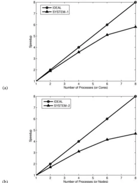
Next, we perform a scalability analysis to analyze the variation of speedup with respect to increments in the number of processes on our available parallel systems, i.e., SYSTEM-1 and SYSTEM-2. Fig. 2(a-b) shows the scalability pattern of speedup for our example problem of moving flame front, solved with K = 160 and N = 8. On SYSTEM-1, which is an 8-core machine, the parallel code exhibits better efficiency when the number of processes (or cores) is less than 8. With the increase in the number of processes, more number of cores is used. This decreases the parallel efficiency, mainly due to the increase in memory bandwidth contention. With 8 processes on the 8 CPU cores, we observe a speed up of 5.68 (71% parallel efficiency).
Fig. 1(a): Temperature and density profiles for the moving flame front problem with K = 80 and N = 4
Fig. 1(c): Temperature and density profiles for the moving flame front problem with K = 80 and N = 8
Fig. 1(d): Temperature and density profiles for the moving flame front problem with K = 80 and N = 10
(a) (b)
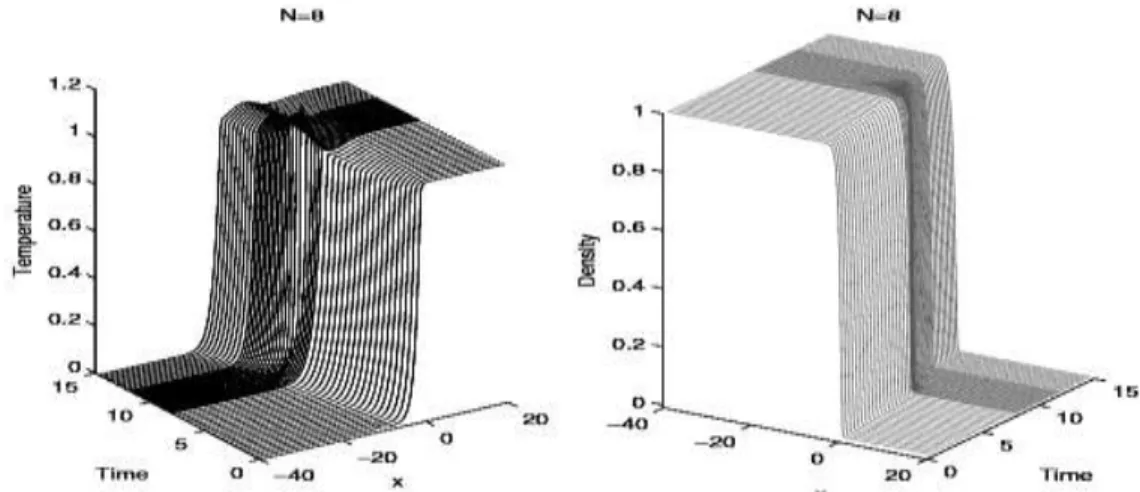
Fig. 3: Temperature and density profiles for Dwyer-Sanders model problem with K = 200 and N = 8
(a)
(b)
On SYSTEM-2, which is an 8-node cluster, 1 process per node is mapped. The parallel code exhibits comparatively lower parallel efficiency (59%). On the cluster, the main parallel overhead is due to the network latency which is because of communication occurring among the processes through Ethernet. For our test case this overhead is vital because of very low computation to communication ratio. The computation to communication ratio increases as we increase the number of elements per process, by using a finer grid.
For the second numerical example, that is based on Dwyer-Sanders flame propagation model, we compute the results using the parallel nodal discontinuous Galerkin code with number of elements K = 200 and polynomial order N = 8. Fig. 3 shows the obtained profiles of temperature T and density Y at selected values of time t. These results are in good agreement with those presented in [17-20]. For this test case, we observe similar scalability pattern of the parallel code as we obtained with the first example problem on our parallel systems, SYSTEM-1 and SYSTEM-2 with number of elements K = 160 and polynomial order N = 8. The comparison is presented in Fig. 4(a-b).
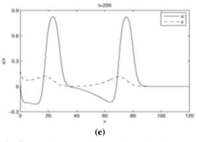
The results for the third numerical example, which is based on Fitzhugh-Nagumo equations of Mathematical Biology, are computed with polynomial order N = 8 using 4 MPI processes on a quadcore CPU based system. The obtained profiles of dependent variables u and v are shown in Fig. 5(a-e) for number of elements K = 80. The results are in good agreement with those presented in [18,19] and especially in [16], which used a moving finite element method with 3rd order approximations in each element. The moving finite element method was introduced in [31,32]. It was used for solving time-dependent partial differential equation in 1D. The CPU time to accomplish the integration was 7.1 hours in [16], while in our case we obtained the nodal discontinuous Galerkin method based solution, with four processes on the quadcore CPU, in about 17 minutes with number of elements K = 120, hence, achieved a remarkable time efficiency.
(a)
(b)
(c)
(e)
Fig. 5: Solution profiles of Fitzhugh-Nagumo equations with K = 80 and N = 8, (a) at t = 40, (b) at t = 80, (c) at t = 120, (d) at t = 160, (e) at t = 200
6. Conclusions
We developed a parallel discontinuous Galerkin code for solving a number of 1D reacting flow problems. Unlike other finite element schemes which are mostly adaptive or moving grid methods for resolving the sharp moving fronts in reacting flows, we obtained the solution by „high order‟ polynomial approximation locally within each element which is the main feature of a discontinuous Galerkin method. We applied the nodal discontinuous Galerkin method with approximating polynomials of orders up to 10 to solve our example problems. We also investigated the performance and scalability of our code on a number of parallel computing systems. Benchmarking of our current implementation on the two systems considered indicates that the upper bound on the performance of this parallel code is due to the network overheads, not due to the memory bandwidth. The current parallel implementation of the nodal discontinuous Galerkin method is intended for stand-alone PCs having a large number of processing cores, and for small clusters of PCs. The successful and efficient implementation of the high order discontinuous Galerkin method (DGM) in the present work is encouraging to consider it for large scale reacting flow simulations.
7. Acknowledgements
We are thankful to Prof. Dr. Amanullah Khan at Institute of Computing, Bahauddin Zakariya University, Multan and Mr. Muhammad Ali Ismail at
Department of Computer and Information System Engineering, NED University, Karachi for their valuable support.
8
References
[1] R. Löhner; Applied Computational Fluid Dynamics Techniques: An Introduction Based on Finite Element Methods, John Wiley & Sons, Chichester, (2008).
[2] J.S. Hesthaven, and T. Warburton; Nodal Discontinuous Galerkin Method: Algorithms, Analysis, and Applications, Springer Texts in Applied Mathematics 54, Springer-Verlag, New York, (2008).
[3] B. Cockburn, G.E. Karniadakis, and C.W. Shu (Eds.); Discontinuous Galerkin Methods: Theory, Computation, and Applications, Lecture Notes in Computational Science and Engineering, vol. 11. Springer-Verlag, New York, (2000).
[4] F. Bassi, and S. Rebay; A high-order accurate discontinuous Galerkin finite element method for the numerical solution of the compressible Navier–Stokes equations, Journal of Computational Physics, 131 (1997) 267–279.
[5] B. Cockburn, and C.W. Shu; The local discontinuous Galerkin method for time-dependent convection–diffusion systems, SIAM Journal on Numerical Analysis, 35 (6) (1998) 2440–2463.
[6] C.E. Baumann, and J.T. Oden, A discontinuous hp finite element method for the Euler and the Navier-Stokes equations, International Journal for Numerical Methods in Fluids, 31 (1) (1999) 79–95.
[7] D.N. Arnold, F. Brezzi, B. Cockburn, and D. Marini, Unified Analysis of discontinuous Galerkin methods for elliptic problems, SIAM Journal on Numerical Analysis, 39 (5) (2002) 1749–1779.
[8] F. Bassi, A. Crivellini, S. Rebay, and M. Savini; Discontinuous Galerkin solution of the
Reynolds-averaged Navie-Stokes and k- turbulence model equations, Computers and Fluids, 34 (2005) 507–540.
[9] B.V. Leer, and S. Nomura; Discontinuous Galerkin for diffusion, 17th AIAA Computational Fluid Dynamics Conference, AIAA-2005-5108 (2005).
[10] M. Dumbser, D.S. Balsara, E.F. Toro, and C.D. Munz; A unified framework for the construction of one-step finite volume and discontinuous Galerkin schemes on unstructured meshes, Journal of Computational Physics, 227 (18) (2008) 8209–8253.
[11] J. Peraire, and P.O. Persson; The compact discontinuous Galerkin (CDG) method for elliptic problems, SIAM Journal on Scientific Computing, 30 (4) (2008) 1806–1824.
[12] H. Luo, J.D. Baum, and R. Löhner; A discontinuous Galerkin method based on a Taylor basis for compressible flows on arbitrary grids, Journal of Computational Physics, 227 (20) (2008) 8875–8893.
[13] Amjad Ali, Hong Luo, Khalid S. Syed, and Muhammad Ishaq; A Parallel Discontinuous Galerkin Code for Compressible Fluid Flows on Unstructured Grids, Journal of Engineering and Applied Sciences, 29 (1), in press.
[14] Hong Luo, Luqing Luo, Amjad Ali, Robert Nourgaliev, and Chunpei Cai; A Parallel, Reconstructed Discontinuous Galerkin Method for the Compressible Flows on Arbitrary Grids,
Communications in Computational Physics, 9(2) (2011), 363–389.
[15] I. Ahmad, and M. Berzins; MOL solvers for hyperbolic PDEs with source terms,
Mathematics and Computer in Simulation. 56(2) (2001) 115–125.
[16] M.C. Coimbra, C. Sereno, and A. Rodrigues; Moving finite element method: applications to science and engineering problems, Computer and Chemical Engineering, 28 (2004) 597–603.
[17] J. Lang, and A. Walter; A finite element method adaptive in space and time for nonlinear reaction-diffusion-systems, IMPACT of Computing in Science and Engineering, 4 (1992) 269–314.
[18] J.I. Ramos; Finite element methods for one-dimensional flame propagation problems, in: T.J. Chung (Eds.), Numerical Modeling in Combustion, Taylor and Francis, Washington, DC, (1993) 3–131.
[19] J.G. Verwer, J.G. Blom, and J.M. Sanz-Serna; An adaptive moving grid method for one-dimensional systems of partial differential equations, Journal of Computational Physics,
82 (2) (1989) 454–486.
[20] A.V. Wouwer, P. Saucez, W.E. Schiesser, and S. Thompson; A MATLAB implementation of upwind finite differences and adaptive grids in the method of lines, Journal of Computational
and Applied Mathematics, 183 (2005) 245–258.
[21] MPICH project.
http://www.mcs.anl.gov/research/projects/mpi/ (last accessed Jan. 10, 2010).
[22] Beowulf Project. http://www.beowulf.org (last accessed Mar. 5, 2009).
[23] M.H. Carpenter, and C. Kennedy; Fourth-order 2N-storage Runge-Kutta schemes, Technical Report NASA TM-109112, NASA Langley Research Center (1994).
[24] H.L. Atkins, and C.W. Shu; Quadrature free implementation of the discontinuous Galerkin method for hyperbolic equations, AIAA Journal, 36(5) (1998) 775–782.
[25] TOP500 project.
http://www.top500.org/stats/list/33/archtype (last accessed Jun. 10, 2010)
[26] A. Klockner, T. Warburton, J. Bridge, and J.S. Hesthaven; Nodal discontinuous Galerkin
methods on graphics processors, Journal of Computational Physics, 228 (21) (2009) 7863– 7882.
[27] A. Baggag, H. Atkins, and D. Keyes; Parallel implementation of the discontinuous Galerkin method, NASA/CR-1999-209546, ICASE Technical Report No. 99–35 (1999).
[28] Grama, A. Gupta, G. Karypis, and V. Kumar; Introduction to Parallel Computing, Second ed., Pearson Education, Singapore, (2003).
[29] N. Peters, and J. Warnatz (Eds.); Numerical methods in laminar flame propagation, Notes on Numerical Fluid Dynamics, vol. 6, Vieweg, Braunschweig, (1982).
[30] H.A. Dwyer, R.J. Kee, and B.R. Sanders; Adaptive grid method for problems in fluid mechanics and heat transfer, AIAA Journal, 18 (10) (1980) 1205–1212.
[31] C. Sereno, A.E. Rodrigues, and J. Villadsen; The moving finite element method with polynomial approximations of any degree,
Computer and Chemical Engineering, 15 (1) (1991) 25–33.