Improved Time Training with Accuracy of Batch Back Propagation Algorithm Via Dynamic Learning Rate and Dynamic Momentum Factor

(1)

ISSN: 2252-8938, DOI: 10.11591/ijai.v7.i4.pp170-178  170

Improved Time Training with Accuracy of Batch Back

Propagation Algorithm Via Dynamic Learning Rate and

Dynamic Momentum Factor

Mohammed Sarhan Al_Duais, Fatma Susilawati. Mohamad

Faculty of Informatics and Computing, Universiti Sultan Zainal Abidin, Terengganu, Malaysia

Article Info ABSTRACT

Article history: Received Jul 11, 2018 Revised Nov 2, 2018 Accepted Nov 26, 2018

The man problem of batch back propagation (BBP) algorithm is slow training and there are several parameters needs to be adjusted manually, also suffers from saturation training. The learning rate and momentum factor are significant parameters for increasing the efficiency of the (BBP). In this study, we created a new dynamic function of each learning rate and momentum facor. We present the DBBPLM algorithm, which trains with a dynamic function for each the learning rate and momentum factor. A Sigmoid function used as activation function. The XOR problem, balance, breast cancer and iris dataset were used as benchmarks for testing the effects of the dynamic DBBPLM algorithm. All the experiments were performed on Matlab 2012 a. The stop training was determined ten power -5. From the experimental results, the DBBPLM algorithm provides superior performance in terms of training, and faster training with higher accuracy compared to the BBP algorithm and with existing works.

Keyword: Accuracy training Batch Back-propagation algorithm

Dynamic learning rate Dynamic momentum factor Speed up Training

Mohammed Sarhan Al_Duais

Faculty of Informatics and Computing, Universiti Sultan Zainal Abidin, Terengganu, Malaysia.

Email: [email protected]

1. INTRODUCTION

The batch BP algorithm is commonly used in many applications including robotics, automation, and weight changes in ANNs [1]. The BP algorithm has led to tremendous breakthroughs in applications involving multilayer perceptions [2]. Gradient descent is commonly used to adjust the weight using a change the error training; however, this approach is not guaranteed to find the global minimum error [3]. The BBP algorithm is accurate in terms of training [4]. The batch BP algorithm is a new style for updating weight, it is widely used in training algorithms as it is accurate for training [5]. It utilizes the gradient descent, which does not ensure to reach the global minimum error because it may result in leading the local minimum [6,7]. Despite the training rate and momentum factor being significant parameters for controlling the updated weight, it is difficult to select the best valueduring training [8]. Generally, there are two techniques for selecting the values for each training rate and momentum factor. The first is set to be a small constant value from interval [1], the second the selected series value from [9]. The learning rate should be sufficiently large to allow for escaping the local minimum [10]. But the biggest value leads to fast training with oscillation error training. To ensure a Suitable learning BP algorithm, the learning rate must be small [11]. Another requirements for speeding up of the batch BBP algorithm is adaptive training rate and momentum factor together [12]. The main problem of BBP algorithm, is slow training, or stuck training around the local minimum and suffers from saturation training [13]. In addition problem of the BP algorithm, several parameters need to be adjusted manually, such as learning rate and momentum factor [14].

(2)

Current work for solving the slow training of the BBP algorithm is through adapting of a some significant parameters, such as learning rate and momentum factor. For these cases many studies has been done such as [15] improved the BP algorithm through two techniques, the training rate and momentum factor, the values of training rate were fixed at different values. The idea of this study is to set the value of training, rate to be large initially, and then to look at the value of error training after iteration. If the error (e) training is increased, the fit produced changes the value of training, rate multiplied by less than one and then recalculated in the original direction. If the iteration error can be reduced, the fit produced changes the value of training rate by multiplied by a constant greater than one, the next iteration is calculated continuously. In [16] compare several techniques for improved BP algorithm. The BP algorithm with adaptive learning rate and momentum factor gave superior accuracy training at 1000 epochs. In [17] modifying the training rate and momentum. The value of the training rate selected depends on the ratio between the new error and the previous error training. The simulation results show an optimization of the training speed and an oscillation reduction duration training. In [18], created dynamic training that consists of multi-steps. The value of the learning rate and momentum factor are set as munaule value. From the experimental results, the improved algorithm was overall efficient, both in visual effect and quality.

The remaining portion of this paper is organized as follows: Section 2 is the materials and method; Section 3 is created the dynamic parameters; Section 4, is experimental results; Section 5 discussion to validate the performance of the improved algorithm; Section 6,evaluate the performance of improve DBBP algorithm.Finally, Section 7 the conclusions.

2. MATERIALS AND METHOD

This kind of this research belongs to the heuristic method. This method is includes the learning rate and momentum factor. To Investigate the aims of this study there are many steps as follows.

2.1. Data set

The data set is very important for verification to improve the BBP algorithm. In this study, all data are taken from UCI Machine Learning Repository through the link https://archive.ics.uci.edu/ml/index.html. All real dataset change to become normization dataset between [0,1]. All data set divided in to two set training set and testing set.

2.2. Neural Network Model

We propose an ANN model, which consist of three-layer neural network that has an input, hidden, and output layer. The input layer is considered to be {

x

1,

x

2,

x

i }, which represents the nodes; the nodes depend on the types or attributes of the data. The hidden layer is made of two layers with four nodes. Whereas the

L

h_and

LL

k_{are the first and second layer respectively.The output layer}

Y

r_{is made of one}

layer with one neuron. Three basis, two of them are used in the hidden and one in the output layer, which is denoted by

u

0j,

v

0k and

w

0r.

v

hj is the weight between neuron h from hidden layer

L

and neuron j from the hidden layer

LL

.

u

ih is the weight between neuron

i

in the input layer and neuron h in the hidden layer. Finally, the sigmoid function is employed as an activation function.

3. CREATED THE DYNAMIC LEARNING RATE AND MOMENTUM FACTOR

The weight update between neuron k from the output layer and neuron j from the hidden layer is as follows:

(

1)

( )

(

1)

jk jk jk jk

w

t

 

w

t

 



w

t

 



w

t



(1)

Where



w

jk

( )

t

is a weight change the weight is updated for each epoch in Equation 1. Speed up training depends on a parameter that affects the updating of the weight. Before going to create the dynamic function for learning rate and momentum factor. The exponential is monotone function, we can create the learning rate as boundary function as follows

(3)

(k sin 2 )E dmic

e



_



(2)

from above the dynamic learning rate



dmic_{. In this case the property of function exponential}

depend on of the value of

k



sin 2

e

.

sin

e

is the boundary function on defining set of e (error training) also

sin

e

has a boundary as

 

1 sin

e



1  

e

[0,1]. The Equation 2, is bounded function. The weight updated under effected boundary of learning rate. To get smooth training and avoid inflation in the gross weight of the added values for momentum factor, the fitting producer through creating dynamic momentum factor and implicate the



dmic_{. Depend above we can created the dynamic momentum factor as follow:}

( sin 2 )

1 sin( [ (1

)]

) sin(

)

dmic

e Y

r

Y

r k E

e













_

(3)

Where the



is the penalty, the



dmic_{is boundary funcation. Insert the Equation 2 and 3 into}

Equation 1, then the weight is updated between any layer as below

( sin 2 )

1 sin( [ (1 )]

( 1) ( ) k E ( ) r r ) si (n ) ( 1)

jk jk e jk k E jk

w t w t w t e Y Y w t

e              (4)

The weighted updated under effected under dynamic learning rate and momentum factor 3.1. Dynamic batch Back propagation (DBBPLM) algorithm

Update Weight Phase, the weights are adjusted simultaneously, as follows

For each output layer , Y, the out put at neuron r, LLj_{the second layer}

( sin 2 )

1

( 1) ( ) ( k E ) [sin( ( (1 ) ) sin( ) ( 1)

jr jr r j r r k E jr

w t w t e LL eY Y w t

e               (5) For bias

( sin 2 )

0 0 ( sin 2 ) 0

1

( 1) ( ) ( E ) [sin( ( (1 ) ) sin( ) ( 1)

r r

k

r

r r k E r

w t w t e e w t

e Y Y              (6)

For each hidden layer

L

h_{i=0,…,n; h=1,…,q} ( sin 2 )

( sin 2 )

1

( 1) ( ) ( E ) [sin( ( (1 ) ) sin( ) ( 1)

ih ih j i r r E i

k

k h

u t w t e x e Y Y u t

e              (7) For bias

( sin 2 )

0 0 ( sin 2 ) 0

1

( 1) ( ) ( E ) [sin( ( (1 ) ) sin( ) ( 1)

h

k

h h r r k E h

u t u t e e Y Y u t

e              (8)

4. EXPERIMENTAL RESULTS

We calculate the accuracy of training as follows [19], Accuracy (%) =1−absolut(Ti−Oi )

UP−LW ∗ 100

where UP=1 and LW=0 are the upper bound and lower bound of the activation function. 4.1. Experiment result of the DBBPLM algorithm with XOR problem

The DBBPLM algorithm is training under effected dynamic learning rate and momentum factor which created in each Equation 2 and 3. Ten experiments has been done and then take the average of time, epoch and accuracy. The result recorded in the Table 1.

(4)

Table 1. Average the Performance of DBBPLM algorithm with XOR

First structure second structure

Ex Time-sec Epoch Accuracy Training Time-sec Epoch Accuracy Training

Av 1.9569 2741 0.9834 1.6267 2832 0.9858

S.D 0.19802 0 0 0.120328 0 0

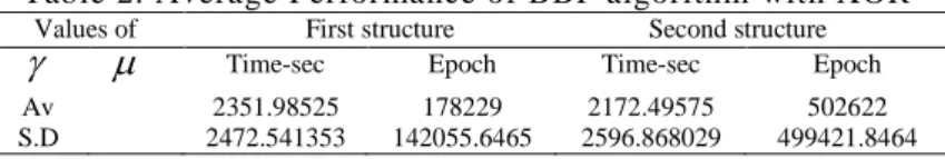
From Table 1, for first structure the average training time is t=1.9569 seconds with 2741 epoch. For second structures the average time training is t=1.6267 seconds, with 2832 epoch. No more different between both structures for accuracy training. The accuracy training is very high for both sturacture. The curve of the training is shown in the following Figure 1.

(a) (b)

Figure 1. Curve Training of Dynamic algorithm with XOR

From Figure 1, the curve (a), is daisy quickly with index epoch to meet global minimum. While the curve (b), the weight training change nearest 1000 epochs, that meaning the DBBPLM algorithm, it has saturation training, but after that, the curve training is converges quickly to obtain the minimum error trianing.

4.2. Experiment result of the BBP algorithm with XOR problem

The BBP algorithm is training with munual value for each learning rate and momentum factor from [0,1]. Eight value for each learning rate and momentum factor were used. The experiment results is recorded in the Table 2.

Table 2. Average Performance of BBP algorithm with XOR

Values of First structure Second structure





Time-sec Epoch Time-sec Epoch

Av 2351.98525 178229 2172.49575 502622

S.D 2472.541353 142055.6465 2596.868029 499421.8464

From Table 2, for first structure the average training time is 2351.98525seconds with178229 epoch. For the second structure, the average training time 2172.49575 second with502622 epoch. The S.D for both structure is greater than one.

4.3. Experiments result of the DBBPLM algorithm with Balance- Training set

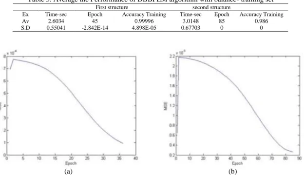
We implement the DBBPLM algorithm using balance-training set. The experiments results is tabulation in the Table 3. From Table 3, for first structure the average training time is 2.6034 seconds with 45 epochs. For second structure the average training time is 3.0148 seconds with epoch is 85 epochs. Both structures gave high accuracy training. The average S.D of time for both structures are less than one. The curve of the training is shown in the Figure 2.

(5)

The training curve of (b) started with flat -spot training, while the curve of training in (a), started without flat spot. The curve (a) attend to the global minimum around 35 epochs, while the curve (b) attend to the global minimum after spend 80 epochs. Also each curve (a) and (b) have different time for training to reach the global minimum.

Table 3. Average the Performance of DBBPLM algorithm with balance- training set

Av 2.6034 45 0.99996 3.0148 85 0.986

S.D 0.55041 -2.842E-14 4.898E-05 0.67703 0 0

(a) (b)

Figure 2. Training curve of the BP algorithm with balance- train

4.3.1. Experiments of the batch BP algorithm with Balance- Traing set

Several value for each



and



were used from ]0,1]. The experiments results are tabulated in Table 4

Table 4. Performance of batch BP algorithm with balance - train set set





Av 1066.545 3416 443.0475 4834

S.D 2025.956102 3577.965095 327.7748629 3431.437717

From Table 4, for first structure, the averge of time is 1066.545



1067 s with average epoch is 3416, while the second structure the averge of time training is 443.0475



443 s with 4838 epoch.

4.3.2. Experiments result of the DBBPLM algorithm with Balance- Testing set The experiments result is tabulated in the Table 5.

Table 5. Average the Performance of DBBPLM with Balance - Testing set

Ex Time – sec Epoch Accuracy Training Time-sec Epoch Accuracy Training

Av 4.6975 92 0.9908 4.5906 104 0.9860

S.D 0.7695144 0 0 0.4191749 0 0

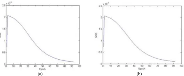
From Table 5, for first structure the average training time is 4.6975seconds at an average epoch of is 92epoch. For second structure the average training time is 4.4850 seconds at an average epoch of is 104

(6)

epoch. Both structures gave high accuracy training. The average S.D of time for both structures are nearst to zero. Both structures gave high accuracy training. The curve of training shown in Figure 3.

(a) (b)

Figure 3. Curve Training of the DBBLM algorithm for Balance- Testing set

4.3.2. Experiments result of the batch BP algorithm with Balance-Testing set

We run the batch BP algorithm with several munal value, and used the balance-testing set. The experiments result recoded in the Table 6.

Table 6. The performance of the training of b atch BP algorithm with Balance -Testing set





Av 2351.596 8672 1811.0055 19096

S.D 2377.327 9175.253381 2043.02911 17835.4912

From Table 6, for first structure the average time training is 2351.596 second with 8672 epoch. For second structure the average time is 1811.0055 seconds with 19096 epoch.

4.3.3. Experiments DBBLM algorithm with Breast -Training set

We will run the DBBLM algorithm, the experience results are given in the Table 7.

Table 7. Average the performance of DBBPLM algorithm with breast.- Training set

Ex Time – sec Epoch Accuracy Training Time-sec Epoch Accuracy Training

Av 2.356 62 0.999 2.3034 59 0.9982

S.D 0.10709621 0 0 0.10685335 0 0

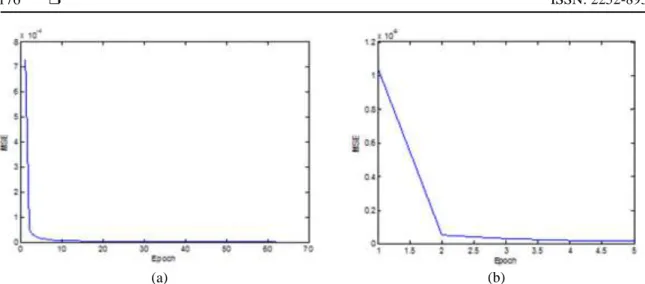
From Table 7, easily can see performance of DBBPLM algorithm. Both the structures the average of the training time is very short. The average S.D of time for both structures are nearst to zero.

(7)

(a) (b)

Figure 4. Curve Training of the DBBLM algorithm for Breast-Training set

Figure 4 from both structure, of the DBBPLM algorithm the training (a) and (b) have smooth curve training. Both Curves are attended fast with index time to the global minimum.

4.3.4. Experiments result of the BBP algorithm with Breast -Training set

We used 374 patterns for training set. The results are shown in the Table 8. From Table 8 for first structure the average time training is 1547.8075 second with 12430 epochs whil second structure the average time is 1361.486667seconds with 15953.

Table 8. Performance of BBP algorithm with Breast -Training set





Av 1547.8075 12430 1361.486667 15953

S.D 2094.247329 18617.69227 1829.096807 15385.18284

4.3.5. Experiments DBBPLM algorithm with Breast-Testing set

From Table 9, the dynamic training rate and momentum factor helps the DBBPLM algorithm for reducing the time training. Both the structures, the average of the training time is very short. For first structure the average time is 0.844seconds with average 33 epochs, while the scond structure the average time is 1.6177with average 61 epochs.

Table 9. Average the performance of DBBPLM algorithm with Breast -Testing set

Av 0.844 33 0.944206 1.6177 61 0.987

S.D 1.1102E-16 0 0 0.09217488 0 0

4.3.6. Experiments results of BBP algorithm with Breast-Testing set

We used 251 patterns for testing the performance of BBP algorithm. The experments result is tabulated in the Table 10.

Table 10. Performance of BBP algorithm with Breast-Testing set





Av 1741.017714 17785.42857 1920.984143 10709

(8)

Form the Table 10, the range of the training time for both structure is 100.3120≤ t ≤6300 seconds and 60.1670 seconds ≤ t ≤4560seconds, this means the range of time training is widely time training

5. DISCUSSION TO VALIDATE THE PERFORMANCE OF IMPROVED ALGORITHM

To validate the efficiency of the improved algorithm, through compare the performance of the DBBPML algorithm with the performance of the batchBP algorithm based on certain criteria. We calculate the speed up training using the following formula [20]:

Speed up = Execution time of 𝐵𝑃 𝑎𝑙𝑔𝑜𝑟𝑖𝑡ℎ𝑚

Execution time of 𝐵𝑃𝐷𝑅𝑀 𝑎𝑙𝑔𝑜𝑟𝑖𝑡ℎ𝑚

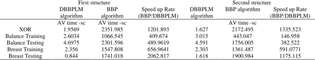
5.1. Proessing Time of DBBPLM Algorithm Versus the BBP Algorithm for with different Structure To validate the improved algorithm or DBBPLM algorithm, we compare the performance between the DBBPLM algorithm and the BBP algorithm. The speed-up obtained in training is shown in Table 11.

Table 11. Speed up the DBBPLM algorithm versus BBP with different structure

First structure Second structure

DBBPLM algorithm

BBP algorithm

Speed up Rate (BBP/DBBPLM)

DBBPLM algorithm

BBP algorithm Speed up Rate

(BBP/DBBPLM)

AV time -sc AV time -sc AV time -sc

XOR 1.9569 2351.985 1201.893 1.627 2172.495 1335.523

Balance Training Balance Testing

2.6034 1066.545 409.674 3.015 443.047 146.958

4.6975 2301.596 489.9619 4.591 1756.005 382.522

Breast Training Breast Testing

2.356 1547.808 656.9641 2.303 1361.487 591.0771

0.844 1741.018 2062.817 1.618 1900.984 1175.115

From Table 11, it is evident that the dynamic algorithm provides superior performance over the BBP algorithm for all datasets with both structure. However for first structure, the DBBPLM algorithm is 2062.817 2063s times faster than the BBP algorithm at maximum training, and also the DBBPLM algorithm is 405.738 406s times faster than the BBP algorithm at minimum training. For second structure The DBBPLM algorithm is 1335.523 1336 times faster than the BBP algorithm at maximum training, and also the DBBPLM algorithm is 146.958 147s times faster than the BBP algorithm at minimum training.

6. EVALUATION OF THE PERFORMANCE OF IMPROVED BATCH BP ALGORITHM

To evaluated the performances of the improved algorithm or DBBPML algorithm for speeding up training which presented in this study. The performances of the DBBPML algorithm are compared to previous research works [13][16]. The performance of the improve algorithm which proposed in this study gives superior performance than exists works.

7. CONCLUSION

This paper introduced the DBBPLM algorithm, which trains by a dynamic function for each the learning rate and momentum factor. This function influences on the weight for each hidden layer and output layer. From experiments resulting the DBBPLM algorithm gives superior training than BBP algorithm for all data set, with both structure. One of the main advantages of the dynamic training is that it reduces the training time and reduces the error training, number of epochs and enhancement the accuracy of the training. The performance of DBBPLM algorithm which presented in this study gave superior performance compare with exists work.

REFERENCES

[1] R.Kalaivani, K.Sudhagar K, Lakshmi P. Neural Network based Vibration Control for Vehicle Active Suspension System. Indian Journal of Science and Technology. 9(1), 2016.

[2] P.Moallem. Improving Back‐Propagation VIA an efficient Combination of A Saturation Suppression Method.

Neural Network World. 20(2), 2010.

[3] l.v Kamble, D.R Pangavhane, & T.P Singh, Improving the Performance of Back-Propagation Training Algorithm by Using ANN. International Journal of Computer, Electrical, Automation, Control and Information Engineering, 9(1), 187-192, 2015.



 

(9)

[4] J.M.Rizwan, PN.Krishnan, R.Karthikeyan, SR.Kumar. Multi layer perception type artificial neural network based traffic control. Indian Journal of Science and Technology, 9(5), 2016.

[5] R. Kalaivani, K. Sudhagar, P. Lakshmi, Neural Network based Vibration Control for Vehicle Active Suspension System. Indian Journal of Science and Technology, 9(1), 2016.

[6] M. S. Al_Duais, & F. S. Mohamad, A Review on Enhancements to Speed up Training of the Batch Back Propagation Algorithm, Indian Journal of Science and Technology, 9(46), 1-10, 2016.

[7] H.. Mo, J.Wang, H. Niu, Exponent back propagation neural network forecasting for financial cross-correlation relationship. Expert Systems with Applications, 53, 106-1016, 2016.

[8] Q.Abbas, F.Ahmad, M.Imran, Variable learning rate based modification in backpropagation algorithm (MBPA) of artificial neural network for data classification. Science International, 28(3), 2369-2378, 2016.

[9] Wu SX, Luo DL, Zhou ZW, Cai JH, Shi YX. A kind of BP neural network algorithm based on grey interval.

International Journal of Systems Science, 42(3), 389-96, 2011.

[10] H. Azami, S.Sanei, Mohammadi K. Improving the neural network training for face recognition using adaptive learning rate, resilient back propagation and conjugate gradient algorithm. Journal of Computer Applications, 34(2):22-6 2011.

[11] J. Ge, J.Sha, & Y.Fang, An new back propagation algorithm with chaotic learning rate. International Conference on Software Engineering and Service Sciences, 16, 404-407, 2015.

[12] J. Gu, G.Yin, P. Huang, J. Guo, L. Chen, An improved back propagation neural network prediction model for subsurface drip irrigation system. Computers and Electrical Engineering, 1-8, 2017.

[13] A.A.Hameed, B. Karlik, M.S.Salman, Back-propagation algorithm with variable adaptive momentum. Knowle dge-Base d Systems, 141, 79–87, 2016.

[14] E.Noersasongko, F. T. Julfia, A. Syukur, R. A. Pramunendar, & C. Supriyanto, Atourism arrival forecasting using genetic algorithm based neural network. Indian Journal of Science and Technology, 9(4), 2016.

[15] W. Zhang, Z.Li, W.Xu, H.Zhou, A classifier of satellite signals based on the back-propagation neural network. In 8th International Congress on Image and Signal Processing (CISP), 1353-1357, 2015.

[16] H..Azami, & J.Escudero, A comparative study of breast cancer diagnosis based on neural network ensemble via improved training algorithms. Proceedings in 37th Annual International Conference of the IEEE Engineering in Medicine and Biology Society (EMBC), 2015, 2836-2839, 2015.

[17] L..Rui, Y. Xiong, Xiao, K., & Qiu, X. BP neural network-based web service selection algorithm in the smart distribution grid. proceedings 16th Asia-Pacific In Network Operations and Management Symposium (APNOMS), 1-4, 2014.

[18] D, Yonghao Z.Peng, YumingS, Sanyuan Z. Improvements of coefficient learning in BPNN for image restoration restoration ICSAI. International Conference on Systems, Yantai, 2692-94, 2012.

[19] N. M, Nawi, N. A Hamid, R. S, Ransing, R,Ghazali & M. N. Salleh, Enhancing Back Propagation Neural Network Algorithm with Adaptive Gain on Classification Problems”. Networks, vol.4, no.2, 2011.

[20] H.Saki, A.Tahmasbi, H. Saltanian-Zadah, aS.B Shokouhi. Fast opposite weight learning rules with application in breast cancer. Computers in biology and medicine. 43(1): 32-41, 2013.