Direct Discrete Method (DDM) and its
Application to Neutron Transport Problems
N. Vosoughi
, A.A. Salehi
1, M. Shahriari
2and M. Heshmatzadeh
1The objective of this paper is to introduce a new direct method for neutronic calculations. This method, called Direct Discrete Method (DDM), is simpler than the Neutron Transport Equation and more compatible with the physical meanings of the problem. The method, based on the physics of the problem, initially runs through meshing of the desired geometry. Next, the balance equation for each mesh interval is written. Considering the connection between the mesh intervals, the nal discrete equation series are directly obtained without the need to rst pass through the set-up of the neutron transport dierential equation. In this paper, a single and multigroup neutron transport discrete equation has been produced for a cylindrical shape fuel element with and without the associated clad and the coolant regions, each with two dierent external boundary conditions. The validity of the results from this new method are tested against the results obtained by the MCNP-4B and the ANISN codes.
INTRODUCTION
A control volume is usually chosen for solving the phys-ical problems on hand and the production, absorption, input and output terms are written for it. Then, if the control volume approaches zero, the relevant dierential equation can be derived. This equation, with its initial and boundary conditions, expresses the mentioned physical phenomena in a mathematical formulation. The derived dierential equation is not usually easy to solve, except for simple and symmetrical geometries. Therefore, numerical methods are bound to be used. In this regard, the continuous parameters must be converted to discrete parameters to produce an algebraic equation series .
RESTRICTIONS IN APPLYING
DIFFERENTIAL EQUATION
Some intricacies in applying the dierential equations have already been stated. Here, some more restrictions in applying this equation are listed [1]:
*. Corresponding Author, National Nuclear Safety Depart-ment, Atomic Energy Organization of Iran, P.O. Box 14155-4494, Tehran, I.R. Iran.
1. Department of Mechanical Engineering, Sharif Univer-sity of Technology, Tehran, I.R. Iran.
2. Faculty of Science, Shahid Beheshti University, P.O. Box 1983-963113, Tehran, I.R. Iran.
1. Physical variables can be classied into two main categories: Global quantities and eld functions. Global quantities are directly measurable in the laboratory; therefore, they must be physical and realizable parameters, such as mass, internal energy and neutron population. The corresponding eld functions are derived from these global variables by a limiting process and are called mass density, energy density and neutron population density. The dierential formulation of physical laws requires the conversion of global variables into eld functions by the limiting process applied to the line, surface and volume to get the densities and to the time interval to get the rates;
2. The analytical solutions of dierential equations are normally possible for smooth boundaries. This con-dition is not commonly met in practice. Therefore, the numerical method is usually used;
3. Usually, sources are concentrated in small regions, like the heat spot of a laser beam or a point neutron source. The dierential formulation leads to con-sidering pointwise concentrated sources, which are unphysical, instead of sources with given intensity concentrated in a small but nite area. In order to overcome this problem, the Dirac generalized function is introduced [2,3];
4. In addition to a few of the mentioned shortcomings attributable to dierential formulations, there is
one other major drawback and that is its infrequent adaptability to analytical solutions. As a result, one should resort to numerical methods, such as the nite dierence method, the nite element method, the weighted residual method and/or the least squares method [4] etc, in order to be able to discretize the dierential equations and, thus, produce a nite set of algebraic equations.
With these introductory remarks, one is now in a position to pose the following questions [5]:
A. Why does one use dierential formulation against all these restrictions and complications?
B. Is dierential formulation the only way to formu-late a physical phenomenon?
C. Is it possible to directly obtain a discrete form of the physical laws without a compulsory passage into the dierential formulation?
The answer to all of these questions, with the notable advance in speed of calculations and the volume of the memory of today's computers, may be given by introducing the new Direct Discrete Method (DDM). This method is much simpler and more compatible with the meanings of physical laws when compared with the customary and widespread dierential formulation method.
GENERAL REMARKS ON DDM
FORMULATION
Three major steps are envisioned to transform the physical problem into the DDM model:
1. Identication of global variable(s) of the specic problem at hand: Dierential formulation uses eld functions, which are spurious and unphysical parameters. DDM uses global variables, which are real and physical parameters. First, the global vari-able(s) should be identied for the dened physical eld. Neutron population is a global variable in a neutronic eld;
2. Adoption of a suitable meshing scheme for the specied geometry: Coordinate systems are the essential tools required to derive and solve dif-ferential equations. In dierential formulation, a coordinate system is usually chosen and, then, the integrals and derivatives are discretized with notice to the chosen coordinate system. As a result, the dierential equations change to a set of algebraic equations. In the DDM method, a suitable meshing scheme should be adopted, such as triangular, rectangular, cylindrical or spherical mesh, depending on the given geometry and its dimensions. For instance, in pin-cell calculations,
it is better to use a cylindrical meshing scheme, considering the fact that fuel elements are usually cylindrical in shape;
3. Formulation of the balance equation for each mesh interval: The balance equation should be written for each of the generated mesh intervals, considering the physics of the problem. Due to the dependence of each mesh interval equation on its neighboring mesh interval equation, the set of the generated DDM equations must, therefore, be solved simul-taneously.
APPLICATION OF DDM TO NEUTRONIC
FIELDS
Neutron population (N) is dened as a global variable
in a neutronic eld. Let one consider a cylindrical mesh element with volume V and surface S. Next,
assume a time interval, t, selected under some special
conditions. The neutron balance equation can now be written for the existing neutrons in this position-time element, based on the events which might happen to these neutrons inside the mesh element.
The following essential assumptions have been made in deriving the neutron discrete equations: 1. One-group energy;
2. Uniform distribution of the materials occupying the regions of the various mesh intervals of the volume element; The dimensions of the mesh intervals are normally so small that this assumption is made acceptable;
3. Uniform distribution of neutron population in each mesh interval;
4. The rates of the entering and exiting neutrons across the various surfaces of the mesh intervals are assumed to be constant;
5. Limit the time interval, t, so as to allow only one
neutron interaction;
6. The static-state case is considered.
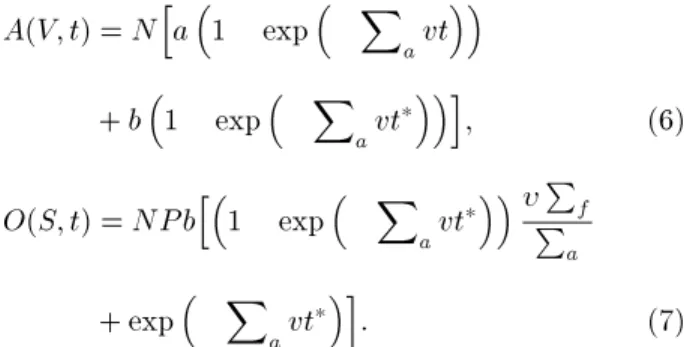
Finally, let one write down the general balance equation, independent of the shape, dimension and material make up of the element under study:
P(V;t) A(V;t) +I(S;t) O(S;t) = 0; (1)
one has, in the above equation:
P: neutron production, A: neutron absorption, I: neutron input, O: neutron output,
V: the volume of the element,
S: the peripheral surface of the element, t: the observation time interval.
Each of the above identied terms will later be explic-itly construed, using the neutronic global variable (N).
DISCRETE FORM OF NEUTRON
TRANSPORT EQUATION IN ONE-GROUP
ENERGY (USING PROBABILITIES)
The above balance equation will be adopted to neu-tronic calculation in this section. To start out, the neutron population shall be divided into two sepa-rate entities, the primary (already available) neutrons within the dierent mesh regions and the secondary (Entrant) neutrons that enter into dierent meshes through their corresponding surfaces. It will be seen, later, that there are, in fact, no substantial dierences between these two groups of neutrons and this division simply becomes handy when deriving the discrete equations.
Primary Neutrons
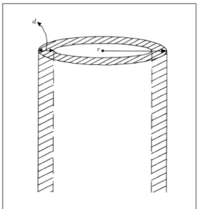
A cylindrical shape fuel element is assumed, with a population of neutrons already inside it. Next, the fate of these neutrons will be investigated during the observation time interval, t. Also, it is assumed that
no neutrons enter the volume through the boundaries at this stage. On the other hand, neutrons set out to move in a certain direction with a nite speed and, by experiencing no interactions, do not necessarily all get the chance to leave the volume element in the nite observation time interval, t. Only neutrons that are
close to the boundary of the element can escape from the volume element. If the speed of neutrons is assigned to be v and the time interval, as already introduced,
is assumed to be t, then, the furthest distance that a
wandering neutron can travel is:
d=vt: (2)
The region realized by this distance, which is adjacent to the surface of every mesh interval, is named the boundary layer thickness (Figure 1). It is obvious that neutrons lying within this boundary layer have the chance of escaping the region. Considering the denition of this boundary layer, the Primary neutrons may be categorized into two dierent groups:
1. Neutrons in the internal zone with an escape prob-ability equal to zero;
2. Neutrons in the boundary layer that have the chance of escaping the region;
Since the neutron population distribution in each mesh interval has already been assumed as uniform, the ratio of neutron population in each of the above mentioned two regions to the total number of neutrons are equal to the ratio of the volume of the respective regions to
Figure 1.
Cylindrical element and its boundary layer.the total volume of the element. Two new parameters,
a (neutrons' internal zone fraction) and b (neutrons'
boundary layer fraction) are dened as:
b= N
b N
=V b V
= [r 2
(r d) 2]
h r
2 h
= d 2+ 2
dr r
2
= 2d r
; (3)
a= N
i N
= V i V
= (r d) 2
h r
2 h
= (r d) 2 r
2
; (4)
where:
N
b: number of neutrons in the boundary layer, V
b: volume of the boundary layer, N
i: number of neutrons in the internal zone, V
i: volume of internal zone,
N: number of total neutrons in the volume element, V: total volume of the volume element.
d
2 is neglected against 2
rd in the above equation.
Consequently, the number of neutrons in the internal zone will be equal toaN and the number of neutrons
in the boundary layer will bebN. Since the boundary
layer neutrons may escape while in their random movement, the average time period available to them is considered ast
, which will be discussed in more detail
in the next section. The following results are obtained for the primary neutrons:
p(V;t) =N j
a
1 exp X
a vt
+b
1 exp X
a vt
k
P
f P
A(V;t) =N h
a
1 exp X
a vt
+b
1 exp X
a vt
i
; (6)
O(S;t) =NPb h
1 exp X
a vt
P
f P
a
+ exp X
a vt
i
: (7)
Calculation of the Neutron Escape Probability
(
P)
A uniform distribution of neutron populations in each volume element and isotropic scattering is assumed. With these remarks in mind, one can imagine that a neutron is located at half distance from the surface of the mesh interval. The fact that the maximum distance that the neutrons can move until they escape from the region isd, which is the radius of a sphere centered at
the point where the escape calculation is to be made (for further clarication refer to Figure 2), then, the escape probability is calculated to be:
P =
2 60 R 0
sind
4 = 14
: (8)
Calculation of the Time Interval (
t) for the
Boundary Layer Neutrons
Since the average time period available to the boundary layer neutrons which do not escape the volume element ist, and the average time period available to the
bound-ary layer neutrons which escape the volume element
Figure 2.
Escape probability calculation for boundary layer neutrons.is t
2, then, one can easily calculate the average time
available to the entire population in that layer, using the above obtained result for the escape probability, as follows:
t
= 14 t
2 + 34t= 7 t
8: (9)
Considering the above result, one can, without any severe approximation and for simplicity, assume t
as
equal tot.
Secondary (Entrant) Neutrons
While this group of neutrons and the primary neutrons hold a lot of similarities, they do, however, dier in two distinct aspects:
1. The primary neutrons have a spatial angle dis-tribution between 0 4 steradian, whereas the
entering neutrons have a direction towards the vol-ume element; therefore, a spatial angle distribution between 0 2 steradian;
2. The average time period available to these neutrons to participate in any reaction within the boundary layer is equal to half of the average time period available to primary neutrons.
Let one identify the entering neutrons into the volume element by the parameter I. Using this parameter,
one can now write down the relevant production, absorption and leakage terms arising from this group of neutrons, as follows:
P i(
V;t) =I
1 exp( X a
v t
2)
P f P
a
; (10)
A i(
V;t) =I
1 exp( X a
v t
2)
; (11)
where the index, i, corresponds to the above dened
parameter,I.
Now, for the calculation of the leakage term, O i,
two groups of neutrons should be considered:
1. The input neutrons, which do not participate in any reaction after entering the volume element. This group of neutrons can travel the maximum distance ofdand then escape the volume element (Figure 3).
Therefore, a fraction of the neutrons that enter from the top of line d and do not participate in any
reaction can escape from the element. Leakage of this group of neutrons would be equal to:
O i1
= 0:197910 13
I: (12)
2. The entrant neutrons, which participate in a scat-tering reaction after enscat-tering the volume element
Figure 3.
Escape probability of neutrons without any reactions.and then escape from it. If the leakage term for this category of neutrons is shown byO
i2; then, by
hindsight and intuition, one can conclude thatO i2
is much smaller thanO i1.
Here, one notes that the contribution of this group of neutrons to the leakage term is very small. It is, therefore, to be deduced that this group of neutrons have only the opportunity to enter the element in the observation time interval t only and that their later
escape can be ignored. However, the nal equation can be written as:
P+P i (
A+A i) (
O+O i1+
O i2) +
I = 0: (13)
Simplication of the Derived Equation
As noted before, the boundary layer thickness is about 10 7meters. Therefore, the derived exponential terms
can be approximated using the Taylor expansion, as follows:
exp( X t
vt) = 1 X
t
vt: (14)
Utilizing this approximation and applying it to the previously derived expressions, the nal equation may be written as:
N X f X a Pb X f X a + 1 vt +I P f P a 2
0:197910 13 vt +O i2 Ivt + 1 vt =0: (15) In the above equation,
P f and
P
a can be ignored
against the 1
vt term in the rst parenthesis and,
likewise, all of the terms in the second bracket against the 1
vt term. With these approximations implemented,
the nal equation becomes:
N X f X a Pb 1 vt +I 1 vt
= 0: (16)
By recalling the expressions obtained forband P and
substituting them in Pb
vt, one gets: Pb vt = 1 4 2d R vt = 12R
: (17)
It is interesting to note that the dimension of the above term is the inverse of the unit of length and shall, henceforth, be dened as Leakage Cross Section (P
L). With this new nomenclature, the nal equation
becomes: N X f X a X L + I vt
= 0: (18)
There are few important observations worth noting in relation to coecient b. The rst observation is
that this coecient is sensitive to the type of external boundary conditions applied; i.e, it depends on using the net current as equal to zero or on putting the incoming current equal to zero. The other important point is that the DDM equation in static-state form for other geometries, such as Slab, Sphere, Square and Triangular [6], are exactly identical, except for their dierences in the coecient, b, indicating its
dependence on the geometry of the volume element.
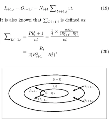
Some Notes on the Input Term (
I)
As seen in Figure 4, the input from mesh volume (i+1)
to mesh volume (i), is the same as the output from
mesh (i+ 1) to mesh (i). As a result, by using the
output term, which was calculated earlier, one obtains the following results:
I i+1;i= O i+1;i= N i+1 X Li+1;i vt: (19)
It is also known thatP
Li+1;i is dened as: X
Li+1;i
= Pb 0 i+ 1 vt = 1 4 2dR i (R 2 i+1 R 2 i ) vt = R i 2(R 2 i+1 R 2 i) ; (20)
where,b 0
i+1 is the inner boundary layer fraction of the
mesh interval (i+ 1). Similarly, the input from mesh
volume (i 1) to mesh volume (i) will be the output
from mesh (i 1) to mesh (i).
It is to be noted that the production, absorption, input and output terms are all stated in terms of the neutronic global variable (N). Deriving the discrete
equations for each of the mesh intervals and linking them together give rise to a series of algebraic equa-tions, which will have to be solved simultaneously. The derived matrix equation isAN = 0, whereAis a (nn)
coecient matrix andNis the unknown (n1) matrix.
Neutron population distribution, the eigenvalue and the corresponding multiplication factor (k) can all be
obtained by solving the matrix equation.
APPLICATION OF THE DDM TO
MULTIGROUP NEUTRON TRANSPORT
EQUATIONS
A cylindrical mesh element with volumeV and surface Sis assumed as a position element, and a time interval, t, is selected the same as one group investigations. All
of the assumed assumptions in one group energy are valid except the neutron population, which depends on energy. However, rather than treat the neutron energy variable, E, as a continuous variable, it will
immediately be discretized into energy intervals or groups. The neutron energy range may be broken into G energy groups, as shown, schematically, in
Figure 5. Notice that a backward indexing scheme was used for energy intervals. Due to the fact that a neutron usually loses energy during its lifetime, neutron up-scattering will be ignored in the pro-cess of neutron multigroup discrete equation produc-tion.
Neutrons in mesh interval (i) and energy group
(g) are assumed and the production and loss of them
will be investigated. These neutrons may be produced by ssion or scattering from other energy groups in mesh interval (i), or, by the escaping of the neutrons
in energy group g from mesh interval (i + 1) and
(i 1) to the desired mesh interval (i). It should be
mentioned that leakage macroscopic cross section does not depend on neutron energy and can be stated by the one-group energy theory. Neutron loss may occur due to absorption, escape or by scattering to other energy groups.
Figure 5.
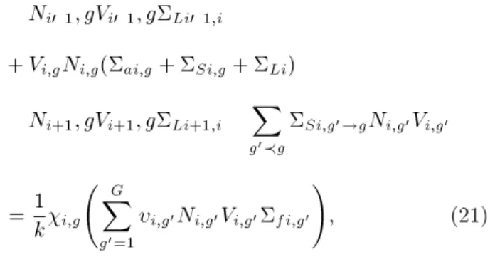
Energy discretizing.Therefore, the nal neutron discrete equation in multigroup energy for mesh interval (i) and energy
groupg, for a cylindrical geometry, becomes: N
i 1 ;gV
i 1 ;g
Li 1;i
+V i;g
N
i;g(ai;g+ Si;g+ Li) N
i+1 ;gV
i+1 ;g
Li+1;i X g
0 g
Si;g 0
!g N
i;g 0
V i;g
0
= 1
k
i;g G X g
0 =1
i;g
0N i;g
0 V
i;g 0
fi;g 0
!
; (21)
where Sig is the total scattering cross section and kis
the multiplication factor of the desired medium. The derived discrete equation can be written in a matrix form,AN =
1 k
BN, whereAandBare ((ng)(ng))
coecient matrices. N is the unknown ((ng)1)
matrix.
RESULTS AND DISCUSSION
To evaluate the DDM method in one-group energy, two typical problems have been solved using the following data (see Table 1). First, a fuel element made up of uranium-235 with a 1 cm radius is considered. Next, a fuel element with the associated clad and coolant regions are considered. The clad and the coolant thicknesses are, respectively, taken as 0.1 cm and 0.3 cm. The type of material assumed for the clad is Zr and that of the coolant is H2O. These examples
are solved for two widespread external boundary con-ditions, namely, J = 0 and Jnet = 0. The same
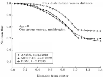
problems have also been solved with the MCNP-4B [8] and the ANISN codes [9]. Figures 6 to 8 show the results for comparison. To evaluate the validity of the DDM method in multigroup energy, two criticality search problems have been solved in the two-group energy. Njoy-97 [10] has been applied to extract
required data from ENDF/B-VI [11] in the two-group energy. The generated data for required elements are presented in Tables 2 and 3. Using the produced two group energy libraries, rst, a fuel element made up of uranium-235 with a 4.8 cm radius (critical radius) is considered. Next, a fuel element with the associated coolant region is considered. The critical radius of the
Table 1.
The data used in the one-group energy test examples [7].Elements
P a
(1/cm)
P f
(1/cm)
P S
(1/cm)
U-235 2.5 3.3e+01 2.8e+01 4.81e-01 Zr 0.00 7.7e-03 0.00 3.03e-01 H2O 0.00 2.26e-02 0.00 2.069
Figure 6.
Neutron ux versus distance for one fuel element with radius of 1 cm in one-group theory (input current into the last mesh is zero).Figure 7.
Neutron ux versus distance for one fuel element associated with clad and coolant in one-group theory (input current into the last mesh is zero).Figure 8.
Neutron ux versus distance for one fuel element associated with clad and coolant in one-group theory (net current into the last mesh is zero).fuel element, which is surrounded by a 6.25 cm coolant, changes to 3.75 cm for the external boundary condition,
J = 0. The same problems have also been solved with
the ANISN code. Figures 9 and 10 show the results for comparison. It should be noticed that the neutron uxes were normalized between 0 and 1. In reality, the thermal ux is in the order of 10 14, in comparison to
order 1 of the fast ux.
CONCLUSION
The DDM method is very simple to set up and obviates the need to go through the dierential formulation process rst. DDM starts from the basic and funda-mental meaning of neutron physics, then, passes to the desired meshing scheme of the geometry at hand and, by writing the balance equation for each mesh interval and combining them, one is nally led to the sought algebraic matrix equation. This method, used for
one-Figure 9.
Neutron ux versus distance for one fuel element with critical radius in two-group theory (input current into the last mesh is zero).Figure 10.
Neutron ux versus distance for a fuel element surrounded by coolant with critical radius in two-group theory (input current into the last mesh is zero).Table 2.
The fast data used in two-group energy test problems.Elements
a1 (Barn)
f1 (Barn)
S1 (Barn)
S1
!1 (Barn)
S1
!2 (Barn)
U-235 1.1865 1.1845 6.386 6.460 1.2E-9 2.85
H-1 3.63E-5 00.00 2.534 2.534 1.3E-6 0.00
O-16 4.00E-2 00.00 2.245 2.245 1.3E-15 0.00
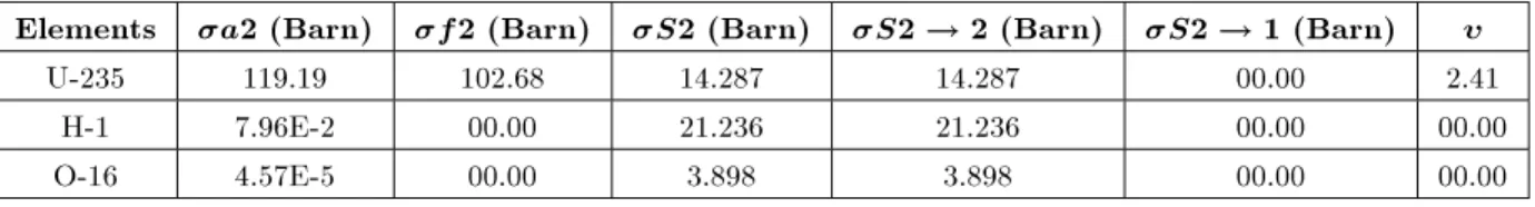
Table 3.
The thermal data used in two-group energy test problems.Elements
a2 (Barn)
f2 (Barn)
S2 (Barn)
S2
!2 (Barn)
S2
!1 (Barn)
U-235 119.19 102.68 14.287 14.287 00.00 2.41
H-1 7.96E-2 00.00 21.236 21.236 00.00 00.00
O-16 4.57E-5 00.00 3.898 3.898 00.00 00.00
group and two-group energy, produces excellent results, which are comparable with those obtained from the MCNP-4B and the ANISN codes.
REFERENCES
1. Tonti, E. \A direct discrete formulation of eld laws: The cell method",CMES,
2
(2), pp 237-258 (2001). 2. Duderstadt, J.J. and Hamilton, L.J.,Nuclear ReactorAnalysis, John Wiley and Sons Inc, New York, USA (1976).
3. Stammler, R.J.J. and Abbate, M.J.,Methods of Steady State Reactor Physics in Nuclear Design, Academic Press (1983).
4. Segerlind, L.J.,Applied Finite Element Analysis, Sec-ond Edition, Agricultural Engineering Department, Michigan State University, John Wiley and Sons (1984).
5. Greenspan, D.,Discrete Numerical Methods in Physics and Engineering, Academic Press (1974).
6. Heshmatzadeh, M. and Salehi, A.A.,A Direct Discrete
Model for The Solution of Neutronic Equations, M.S. Thesis, Sharif University of Technology (1998). 7. Foster, A.R. and Wright, R.L., Basic Nuclear
Engi-neering, Third Edition, Allyn and Bacon, TK 9145 (1977).
8. Briesmeister, J.F. \MCNP-A general Monte Carlo N-particle transport code", Version 4B, Los Alamos National Laboratory Report LA-12625 (1997). 9. Engle, Jr. W.W. \User's manual for ANISN, a
one-dimensional discrete ordinates transport code with anisotropic scattering", Report K-1963, Comput-ing Technology Center, Union Carbide Corporation (1967).
10. Los Alamos National Laboratory, New Mexico, Code System for Producing Pointwise and Multigroup Neu-tron and Photon Cross Sections from ENDF/B Data
(2000).
11. \Members of cross section evaluating working group", Mclane, V., ENDF-102, Data Formats and Proce-dures for the Evaluated Nuclear Data File, ENDF-6, National Nuclear Data Center, Brookhaven National Laboratory (2001).