Sharif University of Technology
Scientia Iranica
Transactions E: Industrial Engineering www.scientiairanica.com
Minimizing maximum earliness in single-machine
scheduling with exible maintenance time
F. Ganji
a, Gh. Moslehi
band B. Ghalebsaz Jeddi
c;a. Department of Industrial Engineering, Golpayegan University of Technology, Golpayegan, P.O. Box 87717-65651, Iran. b. Department of Industrial and Systems Engineering, Isfahan University of Technology, Isfahan, P.O. Box 84156-83111, Iran. c. Faculty of Engineering, Department of Industrial Engineering, Urmia University, Urmia, P.O. Box 57561-15311, Iran. Received 15 August 2015; received in revised form 15 April 2016; accepted 28 June 2016
KEYWORDS Scheduling;
Flexible maintenance; Branch-and-bound; Earliness.
Abstract. We consider minimizing the maximum earliness in the single-machine scheduling problem with exible maintenance. In this problem, preemptive operations are not allowed, the machine should be shut down to perform maintenance, tool changing or resetting takes a constant time, and the time window inside which maintenance should be performed is predened. We show that the problem is NP-hard. Afterward, we propose some dominance properties and an ecient heuristic method to solve the problem. Also, we propose a branch-and-bound algorithm, in which our heuristic method, the lower bound, and the dominance properties are incorporated. The algorithm is computationally examined using 3,840 instances up to 14,000 jobs. The results impressively show that the proposed heuristic algorithm obtains the optimal solution in about 99.5% of the cases using an ordinary processor in a matter of seconds at most.
© 2017 Sharif University of Technology. All rights reserved.
1. Introduction
Nowadays, scheduling problems with availability con-straints have found vast applications in many pro-duction and service systems. Machines and other re-sources may often be unavailable during the scheduling horizon due to breakdown, preventive maintenance, etc. in some time periods. Deterministic machine unavailability problems fall into four categories of: xed unavailability constraint, periodic unavailability constraint, exible maintenance (the subject of our study here), and periodic exible maintenance. In all of these problems, it is assumed that the length of unavailability period or maintenance is known in advance. In scheduling problems, with one or periodic
*. Corresponding author. Tel.: +98 44 3277 5660; Fax: +98 44 3277 3591
E-mail addresses: [email protected] (F. Ganji);
[email protected] (G. Moslehi); [email protected] (B. Ghalebsaz Jeddi)
xed unavailability constraints, it is assumed that the starting time of the unavailability period or periods is determined in advance, but in scheduling problems with a exible maintenance, the starting time of main-tenance(s) is(are) a decision variable(s).
With regard to the single-machine scheduling problems with xed single-period unavailability, Adiri et al. [1] proved that, for the objective of minimizing the total completion time, this problem (i.e. 1; h1kCi)
is NP-hard. Lee and Liman [2] showed that the SPT (Shortest Processing Time) rule for this problem has a tight worst-case error bound of 2/7. Sad et al. [3] proposed an improved version of the SPT rule, called Modied SPT (MSPT), for the same problem, and they proved that the worst-case error bound for their MSPT algorithm is 3/7. Kacem and Chu [4] aimed to minimize the weighted sum of completion times for the problem (i.e. 1; h1kwiCi) and proposed
a branch-and-bound algorithm based on a set of im-proved lower bounds and heuristics. They claimed that their improved algorithm is able to solve instances
of 6000 jobs in a reasonable amount of computation time.
Kacem et al. [5] developed a Mixed Integer Programming (MIP) model for the problem with the objective of minimizing the total completion time (i.e., 1; h1kCi) and used two methods of dynamic
program-ming and a branch-and-bound algorithm. Molaee [6] studied the problem with other separate objectives of minimizing the maximum earliness and minimizing the number of tardy jobs (respectively denoted by 1; h1kEmax and 1; h1kUi). They proposed a heuristic
algorithm and an exact branch-and-bound method to solve 1; h1kEmaxafter showing that the problem is
NP-hard. By proving a number of theorems and lemmas, they developed a lower bound and some ecient dom-inance rules, and so presented heuristic algorithm with O(n log(n)) which was additionally used to calculate the upper bound. Computational results for 2400 instances showed that the branch-and-bound procedure is capable of optimally solving 98.79% of the instances. Then, for 1; h1kUi problem, by proving a number
of theorems, they developed a heuristic procedure to solve the problem. They also proposed a branch-and-bound approach which includes ecient upper and lower bounds and dominance rules. They claimed that \computational results for 2400 problem instances show that the branch-and-bound approach is capable of optimally solving 97.4% of the instances. The proposed heuristic procedure is then evaluated for the problems with large sizes, and it is observed that this procedure has good performance to solve these problems. Results also indicate that the proposed approaches are more ecient when compared to other methods" [6].
Later on, Molaee et al. [7] considered the objec-tives of reference [6] simultaneously (i.e. a bi-criterion objective to simultaneously minimize maximum earli-ness and number of tardy jobs), and they proposed a mathematical optimization model and a branch-and-bound algorithm to solve it.
As for the second group of single-machine schedul-ing problems where we deal with two or more xed periods of unavailability, Liao and Chen [8] considered minimizing the maximum tardiness (i.e. 1; hikTmax) by
providing a heuristic algorithm with O(n2p i)
com-plexity and also by using a branch-and-bound method. Ji et al. [9] considered minimizing the makespan for this class of problems (i.e. 1; hikCmax), and they proved
that the worst case ratio of the classical LPT (Longest Processing Time) algorithm is 2. Chen [10] studied this problem to minimize the number of tardy jobs (i.e. 1; hikUi), and he proposed a branch-and-bound
algorithm as well as a heuristic algorithm to solve it with complexity of O(n2p
i).
The focus of this study is on the single-machine scheduling problem with exible unavailability con-straint (the previously mentioned third group of
scheduling problems). Yang et al. [11] proved that solving the problem to minimize makespan is NP-hard, and they proposed a heuristic algorithm to solve it with complexity of O(n log(n)). Chen [12] studied this problem to minimize the total tardiness (i.e., 1; h1jfajTi) and proposed two mixed Binary Integer
Programming (BIP) models to solve it. Also, Chen [13] proposed two mixed BIP models for this problem with the objective of minimizing the makespan (i.e., 1; h1jfajTmax). In another work, Chen [14] developed
two mixed BIP models for solving 1; h1jfajF problem
to minimize average ow time F for two cases of preemptive (i.e., job splitting is allowed) and non-preemptive jobs.
As for the fourth group of the aforementioned problems, Low et al. [15] considered the single-machine scheduling problem with exible periodic maintenance to minimize the makespan (i.e., 1; hijfpajCmax, where
fpa stands for exible periodic activity/maintenance) and proposed a heuristic algorithm to address it. Qi [16] studied 1; hijfpajCi and 1; hijfpajLmax
prob-lems for the objectives of minimizing the total comple-tion time and maximum lateness, respectively, where the number and the starting time of unavailability constraint are decision variables. They showed that these problems are NP-hard. Sbihi and Varnier [17] presented a heuristic method for the single-machine scheduling problem with several maintenance periods. Specically, two situations were investigated in their study: rst, maintenance periods were periodically xed (i.e. 1; hijpaTmax); second, maintenance periods
were not xed, but the maximum permitted con-tinuous working time of the machine was xed (i.e. 1; hijfpajTmax).
Few researchers have considered the objective of minimizing maximum or total earliness. Such objectives can be appropriate in industries like those producing deteriorative products whose earliness cost can be a major cost of the system. Valente [18] presented a heuristic algorithm for the single-machine scheduling problem to minimize the total weighted earliness (i.e. 1kwiEi). Moslehi and Mahnam [19]
considered the problem of scheduling jobs on a single machine to minimize the sum of maximum earliness and tardiness (i.e. 1kETmax) using ecient lower
and upper bounds and some dominance rules. They also utilized branch-and-bound algorithm for solving the problem. In a more recent study, Moslehi and Rohani [20] considered the single-machine scheduling problem to obtain the Pareto optima for minimizing three objectives of maximum tardiness, maximum ear-liness, and number of tardy jobs using the branch-and-bound algorithm.
In this paper, we consider the single-machine scheduling problem with exible maintenance (with constant duration), and we are to minimize maximum
earliness, Emax, among all earliness, Ei. It is assumed
that there is a xed period inside which maintenance shall be performed, but the starting time of mainte-nance is exible (denoted by fa) and is a decision variable; unforced idle time is not allowed and the jobs are non-preemptive, so the problem is denoted as 1; h1jfajEmax where Emax= max1infEig.
The remainder of the paper is organized as fol-lows: Section 2 elaborates on the problem and presents some lemmas and theorems used to develop solution procedures later on. A heuristic algorithm and a branch-and-bound scheme are presented to solve the problem in Section 3. Section 4 presents numerical examples and computational results to analyze the performance of the heuristic and branch-and-bound algorithms. Section 5 provides the concluding remarks and directions for future studies.
2. Problem properties Notation
Trying to keep it as close as to the notations in the literature (e.g., [21]), we use the following notations throughout the paper:
J Set of all jobs
n Number of jobs
pi (Integer valued) processing time of job
i
di (Integer valued) due date of job i
u The earliest maintenance starting time v The latest maintenance completion
time
W Maintenance interval, i.e. W = v u w Fixed (integer valued) maintenance
time
Ci Completion time of job i
Ei Earliness of job i calculated as
Ei= maxf0; di Cig = (di Ci)+
Si Partial sequence i
p(Si) (Integer valued) processing time of all jobs in Si
si Slack of job i where si= di pi
Set of partial sequence consisting of arranged jobs
0 Set of non-arranged jobs
(complementary set of )
before Group of arranged jobs before the
maintenance
after Group of arranged jobs after the
maintenance whose sequence is known, but their starting time is unknown, and = before[ after
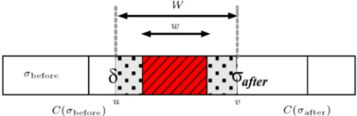
Figure 1. Notional form of the problem at hand.
C() Completion time of any set of jobs, e.g. before or after
Immediate (and the only) idle time before the maintenance
Ei() Earliness of job i in any sequence
Figure 1 depicts the notations of problem 1; h1jfaj
Emax.
The decision variables are the sequence of the jobs, which also denes the starting time of any job and starting time of the maintenance operation.
Major assumptions of the study are as follows: All jobs are of single operation, and preemption or job splitting is not allowed (i.e. jobs are nonpreemptive), and they are simultaneously available at the beginning of the planning horizon; all data are integer including the processing times; unforced idle time is prohibited at any point including before the maintenance (i.e., it is not allowed to create an idle time that can be completely or partially occupied by a job; in other words, < minfpiji 2 afterg); the period [u; v], in
which the maintenance should be performed, has been arranged in advance and clearly maintenance time, w, is smaller than v u.
It is important to note that if an unforced idle time was allowed, all jobs could be processed after the maximum due date with an arbitrary arrangement so that the maximum earliness becomes zero although other criteria, which we do not consider here, may be hurt. However, it is not rational to create such idleness due to the highly valuable machine time.
Furthermore, in the problem at hand, all jobs cannot be processed before the maintenance (i.e., pi > v w); otherwise, the problem reduces to
the case of scheduling without maintenance, where the Minimum Slack Time (MST) sequence is the optimal solution as d[1] p[1] d[2] p[2] d[n] p[n],
where brackets indicate the rankings of the jobs in the sequence [22]. The problem 1; h1jfajEmaxhas not been
addressed in the literature. It is suitable to comment on the complexity of the problem at this point. Molaee [6] showed that the single-machine scheduling problem with a xed unavailability constraint (1; h1kEmax)
along with the assumption of allowed idle time is NP-hard. Thereby, in a particular situation when w = v u, the problem 1; h1jfajEmax converts to
least as much as the complexity of 1; h1kEmax, so the
problem at hand is NP-hard.
In this section, we present a few theorems and lemmas to establish two-solution procedures for the problem. Before discussing the theorems, note that the starting time of jobs in after is not xed since
we do not yet know when the maintenance will start and end; however, we will show that the MST rule is the basis (with some modication) for providing its optimal sequence. Also, note that the starting time of maintenance in this problem is a decision variable so that we cannot assume, by default, that maintenance service starts at rst or ends at the last position of the maintenance time window (in that case, 1; h1jfajEmax
converts to 1; h1kEmax).
Lemma 1: In problem 1; h1jfajEmax, there is an
optimal sequence where jobs in before and jobs in after
are ordered according to MST rule.
Proof: We know that the MST rule is the optimal solution to 1kEmax problem [22]. Jobs are divided
into groups of `before' and `after' maintenance in this problem, where one of them starts processing at time zero (the beginning of the planning horizon) and the other starts right after maintenance. Therefore, each of them shall be ordered with respect to MST rule. Based on this lemma, we introduce some methods here to solve 1; h1jfajEmax problem. The MST
se-quence may generate a feasible sese-quence for 1; h1kEmax
and 1; h1jfajEmax problems; however, care should be
taken because it is not necessarily optimal.
Dominance property 1: Sequences, in which the starting time of a job in before is not in [u; v w], are
a dominant set for 1; h1jfajEmax problem.
Proof: Denote the last job in before by job i, and
if its starting time is in period [u; v w] (and conse-quently, it is completed before v w), then by changing the position of job i and maintenance activity, the completion time of job i increases; therefore, objective function, Emax, will not get worse.
Theorem 1: In the problem 1; h1jfajEmax, MST
sequence is optimal if it generates a feasible solution, no matter where the maintenance is located in [u; v] window, and Emax is of a job from before.
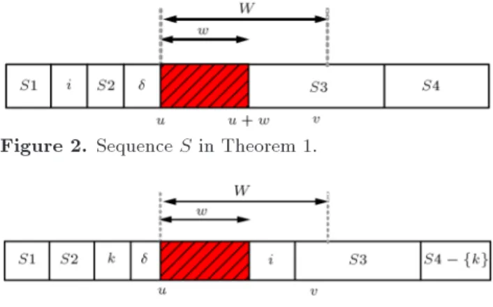
Proof: Denote a feasible solution, S, obtained by MST rule as (S1, i, S2, w, S3, S4) where Emaxis of job
i and Sj is a partial sequence of S, see Figure 2. We shall now show that no replacement decreases Emax.
By exchanging the positions of an arbitrary job from S1 with an arbitrary job from after due to the
Figure 2. Sequence S in Theorem 1.
Figure 3. Sequence S0in Theorem 1.
regularity of MST rule in both before and after , the
replaced jobs are set in the rst position of after and
in the last position of before, respectively. Thereby,
the jobs in set before located after the replaced job in
sequence S are shifted to the left and their starting time decreases; therefore, Emax will not improve.
Additionally, by changing the position of a job from S2 and an arbitrary job from after, Emaxwill not increase
because the starting time of job i has not changed. By exchanging job i with an arbitrary job k from after,
sequence S0 as (S1, S2, k, w, i, S3, S4 fkg) is
obtained, see Figure 3. Without loss of generality, it is assumed that job k is located at the rst position of S4; two situations may occur: the partial sequence, S2, is not empty, or it is empty.
Assume that partial sequence, S2, is not empty and job j is the rst one in S2. Then, the earliness values of jobs i, j, and k in two sequences, S and S0,
after switching jobs k and i are as follows: Ei(S) = maxf(di p(S1) pi); 0g;
Ek(S0) = maxf(dk p(S1) p(S2) pk); 0g;
and:
Ej(S0) = maxf(dj p(S1) pj); 0g;
where, by MST rule, we have di pi dj pj. Thus, by
comparing these relations, we conclude that Ei(S)
Ej(S0).
Now, assume that partial sequence, S2, is empty, so job i is located in the last position of sequence S; thereby, regarding MST rule, we have di pi dk pk.
By comparing the above relations, we arrive at Ei(S)
Ek(S0).
So, the maximum earliness of sequence S is not always greater than this value in sequence S0, then
by switching jobs i and k in sequence S, maximum earliness will not diminish.
Considering the possibility of shifting mainte-nance service back or forth in time, it might be possible to transfer a job from after to before.
Figure 4. Sequence S in Theorem 2.
Figure 5. Sequence S0 in Theorem 2.
Theorem 2: In MST sequence, for 1; h1jfajEmax
problem, if Emax is of a job from after, then the
objective function does not decrease by transferring a job from set after to before.
Proof: The feasible solution, S, is generated by MST rule which is shown as (S1, S2, w, S3, i, S4) and Emax
is related to job i (see Figure 4); regarding feasibility of sequence S, the starting time of jobs in set after
decreases or does not change by transferring a job of set S3 into set beforedue to lling the idle time before
maintenance. Therefore, the objective function does not improve (does not decrease).
Also, by transferring job i into before due to a
decrease in the starting time of job i, the objective function does not improve. Now, assume that a job in S4 is transferred to before. Without loss of generality,
assume that job j is in the rst position of S4; hence, sequence S0 is obtained as (S1, S2, j, w, S3, i, S4
fjg), see Figure 5.
Only job j can aect the maximum earliness in sequence S0, so earliness values of job i in sequence S
and job j in sequence S0 are calculated according to
the following equations:
Ei(S) = maxf(di max(C(before; u)) w
p(S3) pi); 0g;
Ej(S0) = maxf(dj p(S1) p(S2) pj); 0g:
With regard to MST rule, we have di pi dj pj.
Now, by comparing these relations, we obtain Ei(S)
Ej(S0).
Therefore, transferring jobs from after to before
does not improve the objective function.
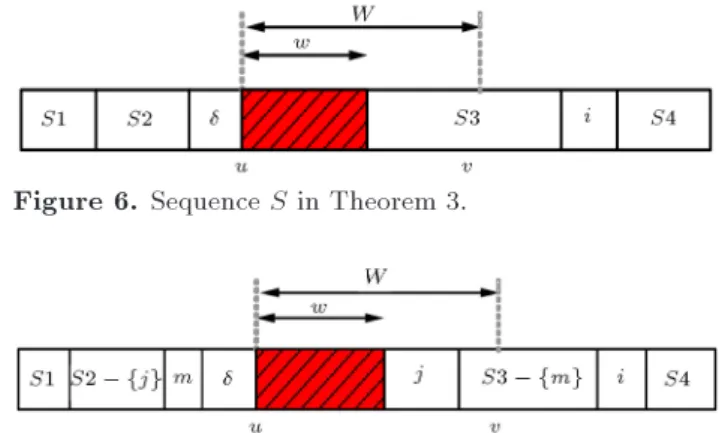
Theorem 3: If the MST rule generates a feasible sequence for 1; h1jfajEmax problem, and Emax
cor-responds to a job (e.g. job i) from after, then this
sequence is optimal only with the following exception: when in the MST sequence, pk < pj where k =
Figure 6. Sequence S in Theorem 3.
Figure 7. Sequence S0 in Theorem 3 and the 2nd
condition.
Arg min
S3 fpg and j = Arg maxbefore
fpg, and exchanging jobs k and j causes the idle time before maintenance to become greater than zero (see Figure 6 for S3). Proof: Assume that Emaxis of a job from after, say
job i. Thus, by switching the positions of an arbitrary job from beforeto an arbitrary job from after, six cases
may occur as follows (Figure 6 shows job i in primary sequence S.):
1. It is obvious that pair-wise replacement of jobs in before (or after) will not lead to any improvement
in the objective function because the MST rule has not been met;
2. By exchanging the positions of jobs m 2 S3 and j 2 before with the assumption of pm pj, sequence
S0 (as S1, S2 fjg, m, w, j, S3 fmg, i, S4) is
obtained, see Figure 7. Due to regularity of MST rule in sets beforeand after, jobs j and m should be
located in the rst position of after and in the last
position of before, respectively. The starting time
of jobs in after, namely job i, does not increase,
and consequently Emax remains unchanged;
3. By exchanging the positions of jobs m 2 S3 and j 2 before with the assumption pm pj, if we
have = 0 after replacement, then the starting time of job i does not change; therefore, Emax will not
decrease;
4. By exchanging the positions of job i with an arbitrary job from before, the starting time of job i
decreases; therefore, the objective function will not improve;
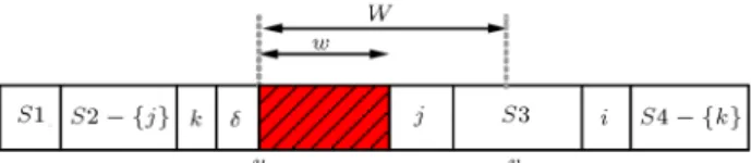
5. By exchanging the positions of jobs k 2 S4 and j 2 before, we obtain sequence S0(as S1, S2 fjg,
k, w, j, S3, i, S4 fkg), see Figure 8.
Therefore, job k shifts to the left and jobs in after may be shifted either to the right or left; in
Figure 8. Sequence S0in Theorem 3 and the 5th
situation.
Ei(S) = maxf(di max(C(before); u) w
p(S3) pi); 0g;
Ek(S0)=maxf(dk p(S1) p(S2)+pj pk); 0g:
By comparing the above relations and taking that into account, due to MST, di pi dk pk,
we obtain Ei(S) Ek(S0). Consequently, the
maximum earliness in sequence S will not be greater than this value in sequence S0.
6. By exchanging positions of job m 2 S3 and job j 2 before under the assumption of pm pj, the
maximum earliness may be decreased if > 0. Generally, in sequence S, by exchanging positions of an arbitrary job from after and a job from before, the
maximum earliness will not improve in all situations except in situation (6). This concludes the Theorem. This implies that the MST sequence is not always the optimal sequence for this problem.
The situations of Theorems 1 and 3 are summa-rized in Table 1.
Now, we present another theorem which provides us with the best possible value for the objective function (i.e., a lower bound), which will be helpful in recognizing the optimal solution.
Theorem 4: In 1; h1kEmaxproblem when h1= v u
(i.e., the machine is unavailable in the whole period of [u; v]), if jobs are arranged based on MST rule where unforced idle time is allowed before maintenance, then its optimal solution is a lower bound for 1; h1jfajEmax
problem.
Proof: Since the maximum earliness is not a regular objective function, it does not get worse if an unforced
idle time is allowed. Thus, if maintenance is considered to cover the whole maintenance period [u; v], then MST sequence can be a lower bound for 1; h1jfajEmax
problem.
Now, having these fundamental theorems, we present an ecient and quick heuristic method, which provides an optimal solution in a good majority of the cases and a well near-optimal solution in the rest of them. Further, we also present a modied branch-and-bound procedure, which obtains the optimal so-lution.
3. Problem solution
3.1. A Heuristic algorithm: Flexible MST In this section, we propose a heuristic algorithm (named Flexible MST or FMST) to tackle the problem at hand. Before discussing the algorithm in detail, it might be useful to provide a brieng of it in advance as follows:
Order all jobs according to MST rule and t the maintenance in a feasible place, and denote this sequence by MST. Using Theorems 1 and 3, check
if the optimality conditions are satised. If so, the problem is solved otherwise,
Obtain the lower bound of the problem according to Theorem 4, and then check if any of the jobs from set after can be performed in the idle time before
maintenance. If this is feasible, check if the objective function is equal to the calculated lower bound; if so, the optimal solution is obtained. Otherwise, The obtained sequence might be the optimal
solu-tion or just a near-optimal solusolu-tion (which would be helpful as an upper bound for the branch-and-bound procedure, explained later in Section 3.2).
3.1.1. The algorithm in detail
The steps of FMST are as follows where asterisk sign (*) identies the optimal value of any variable. - Step 1: Let J be the set of all jobs, i.e. J =
fJ1; J2; ; Jng;
- Step 2: Order and index jobs according to MST rule, and then insert the maintenance operation in
Table 1. Optimal situations of MST sequence (Theorems 1 and 3). Position of job
i = Arg maxfEg Theorem Optimality conditions i 2 before 1 Always true
i 2 after 3
Always true, except when pk< pj where
k = Arg min
S3 fpg and j = Arg maxbefore fpg and > 0 after replacement
between so that it begins at u. Denote this sequence by MST and its objective function by Emax MST;
- Step 3: Set 1 = MST. Let m be a counter
for the number of scheduled jobs after maintenance and m = 1; 2; ; M, where M is the size of set after, created rstly based on the MST schedule; so,
initially, m = 1. Let i = Arg maxfEg. Calculate the idle time before maintenance = u C(before).
Calculate a lower bound for Emax using Theorem 4;
- Step 4: Compare with min
afterfpig. Then, we will
face three situations: a) If < min
afterfpig and if i = Arg maxfEg 2 before,
then we have obtained the optimal solution based on Theorem 1; let =
1and Emax = Emax(1)
and exit; b) If < min
afterfpig and i = Arg maxfEg 2 after, go
to Step 5. But; c) if > min
afterfpig and if it is possible to switch
the rst job of after to the end of before, do so
and start Step 4 from the beginning; otherwise, if switching the rst job of after to the end of
before is not possible, let m = m + 1 and go
to Step 6, unless m = M; in that case, go to Step 11 to exit (Note that at the end of this step, a feasible sequence is obtained.);
- Step 5: Let S3 be a subset of jobs in after
with indices smaller than i in MST sequence (see Figure 6). If pk < pj where k = Arg min
S3 fpg and j =
Arg max
before
fpg, then, according to Theorem 3, swap jobs j with k, update 1and Emax(1), check if new
min
afterfpig, then go to Step 7 if so. Otherwise, the
switching is not possible, and so the optimal solution is obtained; let =
1 and Emax = Emax(1) and
exit;
- Step 6: By starting from job m and checking every job forward, if transferring any job from after to
beforeis possible, add that job into beforeaccording
to MST; note that the other jobs are already in MST sequence. Update . If min
afterfpig, go to Step7;
otherwise let m = m + 1 and continue this process until all jobs in after are checked if they could be
transferred to before;
- Step 7: If Emax() does not correspond to a job
in before, then go to Step 8. Otherwise, if Emax()
corresponds to a job in before, then (because the
MST sequence is now shued) do the following: Let m = m + 1, start from job m in after, if its
transferring to the end of beforeis possible, do so and
transfer the job with maximum earliness in before
into after, slide maintenance forward if necessary
and possible to t the job into before. Update
sequences in beforeand afteraccording to MST rule
separately and calculate .
By selecting and replacing all jobs in after,
the objective function is calculated, and the best sequence among them is selected. If min
afterfpig,
then go to Step 11 to exit; otherwise, let m = m + 1 and go to Step 9;
- Step 8: Let m = i + 1 where i = Arg maxfEg and go to Step 9;
- Step 9: If switching job m to beforeis not possible,
go to Step 10. Otherwise, add job m (a job after i) to before, and then let maintenance in an appropriate
position and update the jobs in before, after and
update . By selecting and replacing every job in after, calculate the objective function and select the
best sequence among them. If min
afterfpig, go to
Step 11 to exit; otherwise, let m = m + 1 and repeat Step 9 from the beginning;
- Step 10: If m = M, the number of jobs in initial after, then go to Step 11 to exit; otherwise, let m =
m + 1 and go to Step 9;
- Step 11: If Emax(1) is equal to the lower bound,
then 1 is optimal, let = 1 and Emax =
Emax(1). Otherwise, a solution is obtained which
still might be optimal or just near optimal (This will be checked by the branch-and-bound algorithm in Section 3.2.). Exit the algorithm.
3.1.2. Computational complexity of FMST
Based on the steps of FMST algorithm, its complexity at Step 2, in which the jobs are ordered according to MST rule, is O(n log(n)). By proceeding in the algorithm and pair-wise replacement of the jobs in Steps 7 and 9, the overall complexity of the proposed FMST is O(n2).
3.2. A branch-and-bound procedure
As shown in the nal step of the FMST algorithm, in some cases, the conditions of Theorems 1 and 3 are not met nor the lower bound of Theorem 4 is reached; therefore, the algorithm could not obtain the optimal solution. In such cases, by having a feasible and near-optimal solution from the FMST algorithm, we proceed with a branch-and-bound procedure to obtain an exact optimal solution for the problem.
An upper bound
The quantity of the objective function returned from execution of the FMST algorithm, which corresponds to a feasible and near-optimal solution, can be regarded as an upper bound for our minimization problem. Having this upper bound will expedite the procedure, and there is a need to calculate a lower bound in every step, as discussed below.
A lower bound
Based on the following theorem, we generate a lower bound for partial sequences of the procedure obtained in every node.
Theorem 5: In partial sequence (consisting of arranged jobs) for 1; h1jfajEmax problem, the lower
bound is given by:
LB() = maxfEmax(); Emax(0)g;
where 0 is the set of non-arranged jobs ordered
ac-cording to MST rule and with the assumption that h1
in 1; h1kEmax problem covers the whole [u; v] window,
i.e., h1= v u.
Proof: It is clear that jobs in 0with arbitrary order
will not aect the objective function of partial sequence . In addition, arranging jobs in 0 based on MST
rule in periods [C(before); u] and [v; 1), assuming
that the unforced idle time is not allowed, yields the minimum value for the maximum earliness. Therefore, the objective function for complete sequence will not be smaller than the aggregate of two values Emax()
and Emax(0).
The branch-and-bound procedure for the problem at hand is as a binary tree consisting nodes and branches, and each node generates two branches based on locating jobs before or after the maintenance win-dow. At rst, before starting the branch-and-bound procedure, jobs shall be ordered and indexed according to the MST rule. In every level, new branches are gen-erated by adding a job from the MST list to the end of the previous jobs before the maintenance if possible (by sliding the maintenance back or force if necessary), or otherwise, to the end of the jobs after the maintenance. Thus, each node provides a partial sequence () for beforeand after. The search strategy in this procedure
is backtracking (namely, the procedure goes through every branch all the way until reaching a fathomed node before moving to another branch at the previous level). The branching continues until all unfathomed branches are visited, or the allowed processing time is over.
The fathoming of a node occurs in three condi-tions:
1. A complete schedule for all jobs is obtained; 2. Lower bound of the partial sequence, LB(),
calcu-lated based on Theorem 5, is greater than the upper bound;
3. A dominated partial sequence is obtained based on the Dominance Property 1.
In the rst case, we update the upper bound if new Emax is less than the current upper bound.
4. Numerical examples and results
To evaluate the performance of the proposed branch-and-bound and FMST algorithms, we code them in C++ and carried out plenty of numerical experiments
on a personal computer with a 3 GB RAM, Core 2Duo, CPU P8400, Pentium 4 under Windows 7 operating system. We generate parameters of test problems as used by Kacem, et al. [5], Yang, et al. [11], and Chen [13] as examples. Our experiment is performed using 16 dierent problem sizes of n 2 f10, 20, 30, 50, 100, 200, 300, 500, 700, 1000, 2000, 4000, 6000, 8000, 12000, 14000g. Processing times, p, are randomly chosen from a discrete uniform distribution over [1; 10], identically done in some other references, e.g. Sbihi and Varnier [17], Liao and Chen [8], and Pathumnakul and Egbelu [23]. Due dates d are uniformly distributed over [(1 C Q=2)pi, (1 C + Q=2)pi], subject
to di pi, where C and Q take values of 0.2 and
0.6. The start of maintenance window, u, is taken as the integer part of 1
4pi, 12pi, and 34pi, subject
to u max1infpig, while the end of maintenance
window is v = u + 30. Maintenance times w are all randomly chosen over w 2 [1; 15] and [16; 30], where v u w.
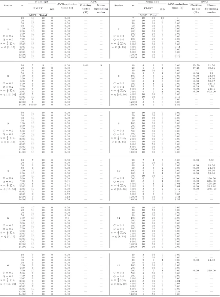
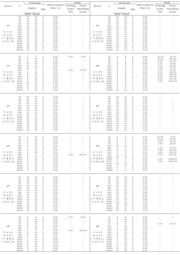
For any problem with n jobs, we run 10 ran-dom sampling (replications) for each combination of parameters. Therefore, a total of 3840(= 10 16 2 2 3 2) test problems are examined in our study. For solving these problems, 3600 seconds of time constraint is applied. Table 2 presents the results, where the column \Num-opt" shows the number of problems that is solved optimally by branch-and-bound or FMST algorithms in less than one hour. Subcolumn \FMST" shows the number of problems that is solved optimally by FMST algorithm composed of two parts of \MST" and \Total". In the MST column, the number of optimally solved problems using Theorems 1 and 3 and the number of optimally solved problems in the \Total" column using the heuristic algorithm are presented. The next subcolumn, titled \BB", shows the number of problems that is solved optimally by branch-and-bound algorithm. Column \Cutting nodes %" shows the average number of cut nodes (because of lower bound and dominance property) relative to all traveled nodes in percent. \0.00" in the lower bound means that the associated problems have reached the optimal solution merely by cutting the rst nodes in less than 0.005 seconds, so they are rounded to 0.00.
Applying the Dominance Property 1 in the struc-ture of branch-and-bound algorithm helps to discard plenty of non-optimal solutions, and consequently the percentage of cutting nodes decreases dramatically. As shown in Table 2, in the series of odd numbers, all the problems were solved optimally without entering
Table 2. Performance of the branch-and-bound and FMST algorithms in 24 series. Series n Num-opt AVG-solution time (s) AVG Series n Num-opt AVG-solution time (s) AVG
FMST BB Cuttingnodes (%)
Num-Spending
nodes
FMST BB Cuttingnodes (%)
Num-Spending
nodes
MST Total MST Total
1
C = 0:2 Q = 0:2 u = 14Ppi
w 2 [1; 15]
10 10 10 0 0.00 | |
7
C = 0:2 Q = 0:6 u = 14Ppi
w 2 [1; 15]
7 10 10 10 0 | |
20 10 10 0 0.00 | | 20 10 10 0 0.00 | |
30 10 10 0 0.00 | | 30 10 10 0 0.00 | |
50 10 10 0 0.00 | | 50 10 10 0 0.00 | |
100 10 10 0 0.00 | | 100 10 10 0 0.00 | |
200 10 10 0 0.00 | | 200 10 10 0 0.00 | |
300 10 10 0 0.00 | | 300 10 10 0 0.00 | |
500 10 10 0 0.00 | | 500 10 10 0 0.00 | |
700 10 10 0 0.00 | | 700 10 10 0 0.00 | |
1000 10 10 0 0.00 | | 1000 10 10 0 0.00 | |
2000 10 10 0 0.00 | | 2000 10 10 0 0.00 | |
4000 10 10 0 0.00 | | 4000 10 10 0 0.11 | |
6000 10 10 0 0.00 | | 6000 10 10 0 0.00 | |
8000 10 10 0 0.00 | | 8000 10 10 0 0.00 | |
12000 10 10 0 0.00 | | 12000 10 10 0 0.10 | {
14000 10 10 0 0.00 | | 14000 10 10 0 0.19 | {
2
C = 0:2 Q = 0:2 u = 14Ppi w 2 [16; 30]
10 7 9 1 0.00 0.00 3
8
C = 0:2 Q = 0:2 u = 14Ppi w 2 [16; 30]
10 8 8 2 0.00 35.70 11.50
20 8 10 0 0.00 | | 20 6 6 4 0.00 77.25 90.75
30 9 10 0 0.00 | | 30 10 10 0 0.00 | |
50 8 10 0 0.00 | | 50 9 9 1 0.00 0.00 13
100 6 10 0 0.00 | | 100 8 8 2 0.00 0.00 23.50
200 7 10 0 0.00 | | 200 9 9 1 0.00 0.00 58.00
300 7 10 0 0.00 | | 300 6 7 3 0.00 0.00 78.67
500 6 10 0 0.00 | | 500 8 8 2 0.00 0.00 127.5
700 7 10 0 0.00 | | 700 9 9 1 0.00 0.03 178
1000 5 10 0 0.00 | | 1000 8 8 2 0.02 0.00 243.5
2000 9 10 0 0.00 | | 2000 9 9 1 0.02 0.00 502.00
4000 5 10 0 0.00 | | 4000 10 10 0 0.00 | |
6000 10 10 0 0.00 | | 6000 10 10 0 0.17 | |
8000 8 10 0 0.00 | | 8000 9 9 0 0.00 | |
12000 8 10 0 0.00 | | 12000 8 8 0 0.00 | |
14000 10000 10 0 0.00 | | 14000 4 5 0 1.87 | |
3
C = 0:2 Q = 0:2 u = 12Ppi
w 2 [1; 15]
10 10 10 0 0.00 | |
9
C = 0:2 Q = 0:6 u = 12Ppi
w 2 [1; 15]
10 10 10 0 0.00 | |
20 10 10 0 0.00 | | 20 10 10 0 0.00 | |
30 10 10 0 0.00 | | 30 10 10 0 0.00 | |
50 10 10 0 0.00 | | 50 10 10 0 0.00 | |
100 10 10 0 0.00 | | 100 10 10 0 0.00 | |
200 10 10 0 0.00 | | 200 10 10 0 0.00 | |
300 10 10 0 0.00 | | 300 10 10 0 0.00 | |
500 10 10 0 0.00 | | 500 10 10 0 0.00 | |
700 10 10 0 0.00 | | 700 10 10 0 0.00 | |
1000 10 10 0 0.00 | | 1000 10 10 0 0.00 | |
2000 10 10 0 0.00 | | 2000 10 10 0 0.00 | |
4000 10 10 0 0.00 | | 4000 10 10 0 0.00 | |
6000 10 10 0 0.00 | | 6000 10 10 0 0.00 | |
8000 10 10 0 0.00 | | 8000 10 10 0 0.00 | |
12000 10 10 0 0.00 | | 12000 10 10 0 0.00 | |
14000 10 10 0 0.00 | | 14000 10 10 0 0.00 | |
4
C = 0:2 Q = 0:2 u = 12Ppi w 2 [16; 30]
10 7 10 0 0.00 | |
10
C = 0:2 Q = 0:6 u = 12Ppi w 2 [16; 30]
10 7 7 3 0.00 0.00 5.30
20 7 10 0 0.00 | | 20 9 10 0 0.00 | |
30 9 10 0 0.00 | | 30 8 8 2 0.00 0.00 15.50
50 9 10 0 0.00 | | 50 8 8 2 0.00 0.00 24.00
100 10 10 0 0.00 | | 100 9 9 1 0.00 0.00 50.00
200 10 10 0 0.00 | | 200 9 9 1 0.00 0.00 99.00
300 10 10 0 0.00 | | 300 10 10 0 0.00 | |
500 5 10 0 0.00 | | 500 6 6 4 0.00 0.00 250.50
700 7 10 0 0.01 | | 700 8 9 1 0.00 0.00 345.00
1000 8 10 0 0.01 | | 1000 7 8 2 0.01 0.00 498.50
2000 8 10 0 0.02 | | 2000 9 9 1 0.01 0.00 99.8.00
4000 10 10 0 0.00 | | 4000 8 8 2 0.12 0.00 1994.50
6000 7 10 0 0.19 | | 6000 6 7 0 0.14 | |
8000 6 10 0 0.32 | | 8000 9 9 0 0.00 | |
12000 7 10 0 1.12 | | 12000 9 10 0 0.41 | |
14000 9 10 0 0.54 | | 14000 7 10 0 1.57 | |
5
C = 0:2 Q = 0:2 u = 34Ppi
w 2 [1; 15]
10 10 10 0 0.00 | |
11
C = 0:2 Q = 0:6 u = 34Ppi
w 2 [1; 15]
10 10 10 0 0.00 | |
20 10 10 0 0.00 | | 20 10 10 0 0.00 | |
30 10 10 0 0.00 | | 30 10 10 0 0.00 | |
50 10 10 0 0.00 | | 50 10 10 0 0.00 | |
100 10 10 0 0.0 | | 100 10 10 0 0.00 | |
200 10 10 0 0.00 | | 200 10 10 0 0.00 | |
300 10 10 0 0.00 | | 300 10 10 0 0.00 | |
500 10 10 0 0.00 | | 500 10 10 0 0.00 | |
700 10 10 0 0.00 | | 700 10 10 0 0.00 | |
1000 10 10 0 0.00 | | 1000 10 10 0 0.00 | |
2000 10 10 0 0.00 | | 2000 10 10 0 0.00 | |
4000 10 10 0 0.00 | | 4000 10 10 0 0.00 | |
6000 10 10 0 0.00 | | 6000 10 10 0 0.00 | |
8000 10 10 0 0.00 | | 8000 10 10 0 0.00 | |
12000 10 10 0 0.00 | | 12000 10 10 0 0.00 | |
14000 10 10 0 0.00 | | 14000 10 10 0 0.00 | |
6
C = 0:2 Q = 0:2 u = 34Ppi w 2 [16; 30]
10 7 10 0 0.00 | |
12
C = 0:2 Q = 0:6 u = 34Ppi w 2 [16; 30]
10 8 10 0 0.00 | |
20 9 10 0 0.00 | | 20 1 10 0 0.00 | |
30 8 10 0 0.00 | | 30 9 9 1 0.00 0.00 24.00
50 9 10 0 0.00 | | 50 9 10 0 0.00 | |
100 8 10 0 0.00 | | 100 9 10 0 0.00 | |
200 6 10 0 0.00 | | 200 8 10 0 0.00 | |
300 10 10 0 0.00 | | 300 7 9 1 0.00 0.00 219.00
500 9 10 0 0.00 | | 500 5 10 0 0.00 | |
700 8 10 0 0.00 | | 700 1 10 0 0.00 | |
1000 9 10 0 0.00 | | 1000 8 10 0 0.00 | |
2000 9 10 0 0.00 | | 2000 8 10 0 0.01 | |
4000 5 10 0 0.00 | | 4000 8 10 0 0.04 | |
6000 7 10 0 0.00 | | 6000 1 10 0 0.00 | |
8000 10 10 0 0.00 | | 8000 6 10 0 0.00 | |
12000 9 10 0 0.00 | | 12000 7 10 0 0.27 | |
Table 2. Performance of the branch-and-bound and FMST algorithms in 24 series (continued). Series n Num-opt AVG-solution time (s) AVG Series n Num-opt AVG-solution time (s) AVG
FMST BB Cuttingnodes (%)
Num-Spending
nodes
FMST BB Cuttingnodes (%)
Num-Spending
nodes
MST Total MST Total
13
C = 0:6 Q = 0:2 u = 14Ppi
w 2 [1; 15]
10 10 10 0 0.00 | |
19
C = 0:6 Q = 0:6 u = 14Ppi
w 2 [1; 15]
10 10 10 0 0.00 | |
20 10 10 0 0.00 | | 20 10 10 0 0.00 | |
30 10 10 0 0.00 | | 30 10 10 0 0.00 | |
50 10 10 0 0.00 | | 50 10 10 0 0.00 | |
100 10 10 0 0.00 | | 100 10 10 0 0.00 | |
200 10 10 0 0.00 | | 200 10 10 0 0.00 | |
300 10 10 0 0.00 | | 300 10 10 0 0.00 | |
500 10 10 0 0.00 | | 500 10 10 0 0.00 | |
700 10 10 0 0.00 | | 700 10 10 0 0.00 | |
1000 10 10 0 0.00 | | 1000 10 10 0 0.00 | |
2000 10 10 0 0.00 | | 2000 10 10 0 0.00 | |
4000 10 10 0 0.00 | | 4000 10 10 0 0.00 | |
6000 10 10 0 0.00 | | 6000 10 10 0 0.00 | |
8000 10 10 0 0.00 | | 8000 10 10 0 0.00 | |
12000 10 10 0 0.00 | | 12000 10 10 0 0.00 | |
14000 10 10 0 0.00 | | 14000 10 10 0 0.00 | |
14
C = 0:6 Q = 0:2 u = 14Ppi w 2 [16; 30]
10 7 7 3 0.00 0.00 7.00
20
C = 0:6 Q = 0:6 u = 14Ppi w 2 [16; 30]
10 8 8 2 0.00 52.20 23.00
20 9 10 0 0.00 | | 20 7 7 3 0.00 30.10 270.00
30 8 10 0 0.00 | | 30 7 7 3 0.00 0.00 26.00
50 10 10 0 0.00 | | 50 8 8 2 0.00 0.00 14.00
100 10 10 0 0.00 | | 100 9 9 1 0.00 0.00 25.00
200 10 10 0 0.00 | | 200 9 9 1 0.00 0.00 67.00
300 7 9 1 0.00 0.00 70.00 300 8 8 2 0.00 0.00 78.50
500 6 10 0 0.01 | | 500 6 6 4 0.00 0.00 128.75
700 8 10 0 0.00 | | 700 9 9 1 0.00 0.00 169.00
1000 9 10 0 0.01 | | 1000 8 8 2 0.01 0.00 253.00
2000 8 10 0 0.03 | | 2000 9 9 1 0.02 0.00 501.00
4000 9 10 0 0.07 | | 4000 9 9 1 0.06 0.00 1005.00
6000 10 10 0 0.00 | | 6000 9 9 1 0.00 | |
8000 4 10 0 1.25 | | 8000 9 9 1 0.00 | |
12000 8 10 0 0.87 | | 12000 9 9 1 0.00 | |
14000 9 10 0 0.90 | | 14000 10 10 0 0.00 | |
15
C = 0:6 Q = 0:2 u = 12Ppi
w 2 [1; 15]
10 10 10 0 0.00 | |
21
C = 0:6 Q = 0:6 u = 12Ppi
w 2 [1; 15]
10 10 10 0 0.00 | |
20 10 10 0 0.00 | | 20 10 10 0 0.00 | |
30 10 10 0 0.00 | | 30 10 10 0 0.00 | |
50 10 10 0 0.00 | | 50 10 10 0 0.00 | |
100 10 10 0 0.00 | | 100 10 10 0 0.00 | |
200 10 10 0 0.00 | | 200 10 10 0 0.00 | |
300 10 10 0 0.00 | | 300 10 10 0 0.00 | |
500 10 10 0 0.00 | | 500 10 10 0 0.00 | |
700 10 10 0 0.00 | | 700 10 10 0 0.00 | |
1000 10 10 0 0.00 | | 1000 10 10 0 0.00 | |
2000 10 10 0 0.00 | | 2000 10 10 0 0.00 | |
4000 10 10 0 0.00 | | 4000 10 10 0 0.00 | |
6000 10 10 0 0.00 | | 6000 10 10 0 0.00 | |
8000 10 10 0 0.00 | | 8000 10 10 0 0.00 | |
12000 10 10 0 0.00 | | 12000 10 10 0 0.00 | |
14000 10 10 0 0.00 | | 14000 10 10 0 0.00 | |
16
C = 0:6 Q = 0:2 u = 14Ppi w 2 [16; 30]
10 8 10 0 0.00 | |
22
C = 0:6 Q = 0:6 u = 12Ppi w 2 [16; 30]
10 7 7 3 0.00 12.96 8.00
20 7 10 0 0.00 | | 20 9 9 1 0.00 35.40 48.00
30 9 10 0 0.00 | | 30 9 9 1 0.00 0.00 14.00
50 7 10 0 0.00 | | 50 7 7 3 0.00 0.00 26.00
100 9 10 0 0.00 | | 100 10 10 0 0.00 | |
200 1 10 0 0.00 | | 200 9 9 1 0.00 0.00 96.00
300 9 10 0 0.00 | | 300 8 8 2 0.00 0.00 152.00
500 8 10 0 0.00 | | 500 9 9 1 0.00 0.00 250.00
700 6 9 1 0.00 0.00 353.00 700 9 9 1 0.00 0.00 351.00
1000 9 10 0 0.00 | | 1000 10 10 0 0.00 | |
2000 9 10 0 0.01 | | 2000 8 8 2 0.03 0.00 1009.50
4000 7 10 0 0.06 | | 4000 9 9 1 0.05 0.00 2010.00
6000 9 10 0 0.08 | | 6000 10 10 0 0.00 | |
8000 9 10 0 0.08 | | 8000 7 7 0 0.00 | |
12000 9 10 0 0.13 { | 12000 7 7 0 0.39 | |
14000 9 10 0 0.42 | | 14000 9 9 0 0.55 | |
17
C = 0:6 Q = 0:2 u = 34Ppi
w 2 [1; 15]
10 10 10 0 0.00 | |
23
C = 0:6 Q = 0:6 u = 12Ppi
w 2 [1; 15]
10 10 10 0 0.00 | |
20 10 10 0 0.00 | | 20 10 10 0 0.00 | |
30 10 10 0 0.00 | | 30 10 10 0 0.00 | |
50 10 10 0 0.00 | | 50 10 10 0 0.00 | |
100 10 10 0 0.00 | | 100 10 10 0 0.00 | |
200 10 10 0 0.00 | | 200 10 10 0 0.00 | |
300 10 10 0 0.00 | | 300 10 10 0 0.00 | |
500 10 10 0 0.00 | | 500 10 10 0 0.00 | |
700 10 10 0 0.00 | | 700 10 10 0 0.00 | |
1000 10 10 0 0.00 | | 1000 10 10 0 0.00 | |
2000 10 10 0 0.00 | | 2000 10 10 0 0.00 | |
4000 10 10 0 0.00 | | 4000 10 10 0 0.00 | |
6000 10 10 0 0.00 | | 6000 10 10 0 0.00 | |
8000 10 10 0 0.00 | | 8000 10 10 0 0.00 | |
12000 10 10 0 0.00 | | 12000 10 10 0 0.00 | |
14000 10 10 0 0.00 | | 14000 10 10 0 0.00 | |
18
C = 0:6 Q = 0:2 u = 34Ppi w 2 [16; 30]
10 8 9 1 0.00 0.00 8.00
24
C = 0:6 Q = 0:6 u = 12Ppi
w 2 [1; 15]
10 9 10 0 0.00 | |
20 9 10 0 0.00 | | 20 9 10 0 0.00 | |
30 9 10 0 0.00 | | 30 1 10 0 0.00 | |
50 6 10 0 0.00 | | 50 8 9 1 0.00 0.00 41.00
100 8 10 0 0.00 | | 100 1 10 0 0.00 | |
200 8 10 0 0.01 | | 200 8 10 0 0.00 | |
300 7 9 1 0.00 0.00 224.00 300 5 10 0 0.00 | |
500 8 10 0 0.00 | | 500 8 10 0 0.00 | |
700 8 10 0 0.00 | | 700 8 10 0 0.00 | |
1000 1 10 0 0.00 | | 1000 7 10 0 0.00 | |
2000 1 10 0 0.00 | | 2000 1 10 0 0.00 | |
4000 8 10 0 0.04 | | 4000 1 10 0 0.00 | |
6000 8 10 0 0.10 | | 6000 9 10 0 0.06 | |
8000 9 10 0 0.03 | | 8000 9 10 0 0.04 | |
12000 9 10 0 0.09 | | 12000 10 10 0 0.00 | |
the branch-and-bound algorithm, and also satisfactory results were obtained for the rest of the series. Among these 24 series, 99.48% (i.e., 3820 out of 3840) of the problems were solved optimally in a matter of a couple of seconds at most.
In the series of odd numbers, the ability of FMST algorithm to obtain the optimal solution is very high. This might be due to their short-time maintenance activity, and consequently high otation in these series. Larger u in even series leads to decreasing the number of early jobs in after at the optimal solution, and very
likely, the maximum earliness is obtained from the jobs in before. Thereby, for large u, it is likely that in MST
sequence, the job with maximum earliness is located before the maintenance. Thus, due to the large value of u, the number of problems that is optimal based on Theorem 1 increases, and also probability of eect of switching a job from after to before on maximum
earliness decreases.
In series 2, 8, 14, and 20 where u possesses the least value, 81.87% of 640 problems were solved optimally by Theorem 1, 10.81% by FMST algorithm, and 7.31% by branch-and-bound algorithm. In these series, 1.71% of the problems were left unsolved. It is seen in Figure 9 that the performance of the heuristic algorithm is higher for larger u. So, in series 6, 12, 18, and 24 where u has the highest value, eciency of the heuristic algorithm has taken its highest value; in these series, it can solve 99.21% of the problems optimally, and the proportion of the times used by the branch-and-bound procedure is 0.78%.
From Table 2, we also observe that the solution time, among the problems whose optimal solutions were achieved, has minor changes in terms of u (see the series 1, 2, 7, 8, 13, 14, 19, 20 for u = 1
4pi, series
3, 4, 9, 10, 15, 16, 21, and 22 for u = 1
2pi, and series
5, 6, 11, 12 17, 18, 23, and 24 for u=3 4pi).
It is important to further observe how changes in w aect the time until reaching the optimal solution. According to Table 2, in the series of odd numbers, (i.e., 1; 3; ; 23) where w is in [1; 15], all problems were solved in less than 0.005 seconds on average on
Figure 9. Performances of branch-and-bound and FMST algorithms in terms of u.
all problems in each set. On the other hand, in the series of even numbers, (i.e., 2; 4; ; 24) where w is in [16; 30], six of these problem sets were solved in less than 0.005 seconds on average on all problems in each set, and six other series were solved between 0.006 and 0.025 seconds. We note that the processing time is not meaningfully sensitive to such changes in w.
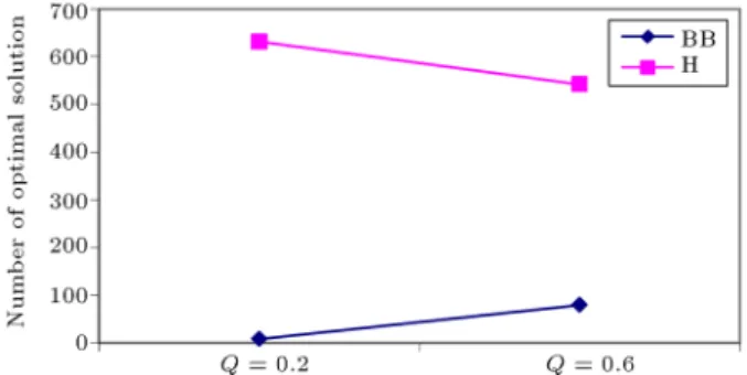
Analyzing the performance of FMST and branch-and-bound algorithms in terms of the range of due dates or Q shows that increasing Q expands upper bound for due date; hence, the number of early jobs in these problems increases. Even the maximum earliness can be related to the jobs in after, and this fact results
in going through more branches of the branch-and-bound tree. For this reason, the performance of the heuristic algorithm is decreased by increasing Q. As it is depicted in Figure 10, in series 2, 4, 6, 14, 16, 18 of Table 2 where Q = 0:2, the eciency of heuristic algorithm is higher than that in series 8, 10, 12, 20, 22, and 24 with Q = 0:6. In the series of Q = 0:2, the following fractions of the tested problems (out of 640 problems) are solved optimally: 71.83% using Theorem 1, 26.91% using FMST algorithm, and 1.25% using branch-and-bound algorithm. A tiny fraction of 0.16% of these problems was left unsolved using our methods. Also, in the series of Q = 0:6, the following fractions of the test problems are solved optimally out of 640 problems: 76.97% by Theorem 1, 10.30% by FMST algorithm, and 12.72% by branch-and-bound algorithm. In these series, 2.97% of the problems were left unsolved.
Referring to Figure 10, it is concluded that by increasing Q, because the number of early jobs increases, more problems enter into the branch-and-bound algorithm and more branches are visited. It is worth mentioning that the branch-and-bound algo-rithm subjected to time constraint in dierent series is not capable of solving some problems with the size of 6,000 jobs or more. Generally speaking, we observe that the problem series with higher values of w and Q and lower values of u are more dicult to solve than the other series.
Figure 10. Performance of branch-and-bound and FMST algorithms in terms of Q.
5. Conclusion
In this paper, the scheduling problem for a single machine with a exible maintenance to minimize the maximum earliness was considered. In this problem, we let the starting time of maintenance be a decision variable inside a specied time window. All jobs were nonpreemptive and no unforced idle time was allowed. First, we showed that it is an NP-hard problem. Then, we proved several theorems and developed a heuristic algorithm (denoted by FMST) to solve it. Also, we proposed a branch-and-bound algorithm along with a lower bound and ecient dominance rule. In this approach, the FMST algorithm was applied as the upper bound. 3840 classic test problems in the form of 24 series were generated and solved using the aforementioned algorithms. Computational results demonstrated that 97.18% and 2.29% of the problems were solved optimally by FMST and the branch-and-bound algorithms, respectively, at most in a matter of seconds; however, a tiny proportion of 0.52% of the problems could not be solved. Based on the results of standard test problems solved here, some sensitivity analyses on the performance of the proposed methods in terms of maintenance time, duration, and starting time of the allowed maintenance window were presented.
References
1. Adiri, I., Bruno, J., Frostig, E. and Rinnoy Kan, A.H.G. \Single machine ow-time scheduling with a single breakdown", Acta Information, 26, pp. 679-696 (1989).
2. Lee, C.Y. and Liman, S.D. \Single machine ow-time scheduling with scheduled maintenance", Acta Information, 29, pp. 375-382 (1992).
3. Sad, C., Penz, B., Rapine, C., Blazevicz, J. and For-manowicz, P. \An improved approximation algorithm for the single machine total completion time schedul-ing problem with availability constraints", European Journal of Operational Research, 161, pp. 3-10 (2005).
4. Kacem, I. and Chu, C. \Ecient branch-and-bound algorithm for minimizing the weighted sum of comple-tion times on a single machine with one availability constraint", International Journal of Production Eco-nomics, 112, pp. 138-150 (2008).
5. Kacem, I., Chu, C. and Souissi, A. \Single-machine scheduling with an availability constraint to minimize the weighted sum of the completion times", Computers and Operations Research, 35, pp. 827-844 (2008).
6. Molaee, E. \Single machine scheduling problem with availability constraint", M.S Thesis, Department of In-dustrial and Systems Engineering, Isfahan University of Technology, Isfahan, Iran (2009).
7. Molaee, E., Moslehi, G. and Reisi, M. \Minimizing maximum earliness and number of tardy jobs in the
single machine scheduling problem", Computers and Mathematics with Applications, 60, pp. 2909-2919 (2010).
8. Liao, C.J. and Chen, W.J. \Single-machine scheduling with periodic maintenance and nonresumable jobs", Computers and Operations Research, 30, pp. 1335-1347 (2003).
9. Ji, M., He, Y. and Cheng, T.C.E. \Single-machine scheduling with periodic maintenance to minimize makespan", Computers and Operations Research, 34, pp. 1764-1770 (2007).
10. Chen, W.J. \Minimizing number of tardy jobs on a single machine subject to periodic maintenance", Omega, 37, pp. 591-599 (2009).
11. Yang, D.L., Hung, C.L., Hsu, C.J. and Chen, M.S. \Minimizing the makespan in a single machine schedul-ing problem with a exible maintenance", J. Chinese Inst. Insyst. Eng., 19, pp. 63-66 (2002).
12. Chen, J.S. \Optimization models for the machine scheduling problem with a single exible maintenance activity", Engineering Optimization, 38, pp. 53-71 (2006).
13. Chen, J.S. \Scheduling of nonresumable jobs and exible maintenance activities on a single machine to minimize makespan", European Journal of Operational Research, 190, pp. 90-102 (2008).
14. Chen, J.S. \Using integer programming to solve the machine scheduling problem with a exible mainte-nance activity", Journal of Statistics and Management Systems, 9, pp. 87-104 (2006).
15. Low, C., Ji, M., Hsu, C.J. and Su, C.T. \Minimizing the makespan in a single machine scheduling prob-lems with exible and periodic maintenance", Applied Mathematical Modelling, 34(2), pp. 334-342 (2009).
16. Qi, X. \A note on worst-case performance of heuristics for maintenance scheduling problems", Discrete Ap-plied Mathematics, 155, pp. 416-422 (2007).
17. Sbihi, M. and Varnier, C. \Single-machine scheduling with periodic and exible periodic maintenance to min-imize maximum tardiness", Computers and Industrial Engineering, 55, pp. 830-840 (2008).
18. Valente, J.M.S. \Local and global dominance condi-tions for the weighted earliness scheduling problem with no idle time", Computers and Industrial Engi-neering, 51, pp. 765-780 (2006).
19. Moslehi, G. and Mahnam, M. \A branch-and-bound algorithm to minimize the sum of maximum earliness and tardiness in the single machine", International Journal of Operational Research, 4, pp. 458-483 (2010).
20. Moslehi, G. and Rohani, M. \Finding Pareto optima for maximum tardiness, maximum earliness and num-ber of tardy jobs", International Journal of Opera-tional Research, 14(4), pp. 433-452 (2012).
21. Pinedo, M.L., Scheduling: Theory, Algorithms, and Systems, 4th Edn., Prentice Hall (2012).
22. Baker, K.R. and Trietsch, D., Principals of Sequencing and Scheduling, John Wiley and Sons, Inc., New York (2009).
23. Pathumnakul, S. and Egbelu, P.J. \Algorithm for min-imizing weighted earliness penalty in single-machine problem", European Journal of Operational Research, 161, pp. 780-796 (2005).
Biographies
Fatemeh Ganji is an Instructor at the Department of Industrial Engineering at Golpayegan University of Technology, Iran. She obtained her Bachelor's degree in Industrial Engineering from Golpayegan University of Technology, and Master's degree in Operations Research from Isfahan University of Technology, Iran. Her main lines of research are production planning, scheduling and sequencing, and design of industrial systems. Besides teaching and research, she has been involved in many projects in industry.
Ghasem Moslehi is an Associate Professor at the Department of Industrial and Systems Engineering, Isfahan University of Technology, Isfahan, Iran. He obtained a Bachelor's degree in Industrial Engineering,
a Master's degree in Operations Research from Isfahan University of Technology, Iran, and a PhD in Indus-trial Engineering from Tarbiat Modarres University, Tehran, Iran. His main lines of research interests are scheduling and sequencing, production planning, and engineering economy. Dr. Moslehi has supervised many MSc and Doctorate thesis, published more than 100 refereed papers in those elds, and also participated in numerous international conferences.
Babak Ghalebsaz Jeddi is an Assistant Professor at the Faculty of Engineering, Urmia University, Iran. He previously lectured at Sharif University of Tech-nology, Iran. He received his BSc degree in Industrial Engineering from Sharif University of Technology, Iran, and MSc degrees from Tehran University, Iran, and University of Cincinnati, Ohio. His PhD degree is con-ferred at George Mason University, Virginia, from the Department of Systems Engineering and Operations Research. His academic interests lie in applied side of operation research, systems engineering, statistics, and microeconomics in areas such as inventory and production control, air transportation system analysis, time series analysis and forecasting, quality control, and mobile network optimization.